State-of-Health Prediction for Lithium-Ion Batteries Based on a Novel Hybrid Approach

Abstract

Generally, the State-of-Health (SOH) monitoring and Remaining Useful Life (RUL) prediction and assessment of lithium-ion (Li-ion) batteries need to use sensors to obtain the degradation test data of the same type of batteries and establish the degradation model for reference. However, when the battery type is unknown, a usable reference model cannot be obtained, so its prediction and evaluation may be relatively inconvenient. In this paper, the State of-Health prediction for lithium-ion batteries based on a novel hybrid scheme is proposed. Firstly, historical charge/discharge time series and capacity series are extracted to analyze and construct Health Indicators, then using Complete Ensemble Empirical Mode Decomposition with Adaptive Noise (CEEMDAN) to decompose the Health Indicator series into the trend and non-trend terms. Among them, the relatively smooth trend item data series uses the Autoregressive Integrated Moving Average model (ARIMA) for prediction; when dealing with the data series of non-trend items which are obviously non-smooth and seemingly random, the residuals predicted by ARIMA and the non-trend items obtained by CEEMDAN decomposition are combined into new non-trend items; then the least square support vector machine (LSSVM) is introduced to build a nonlinear prediction model and make predictions. Finally, combining the prediction results of the trend item data series and the non-trend item data series as a reference for the assessment of the state of health and remaining useful life. The 13 experimental results of 3 batteries verify the effectiveness of the scheme.

1. Introduction

Lithium batteries have a high energy density, easy to use, and can be repeatedly used for charging and discharging, so they are widely used in various equipment such as automobiles, mobile phones, drones, etc. Therefore, the monitoring of its deterioration state and the evaluation of the performance are essential. But lithium batteries rely on the chemical reaction of its internal materials to convert electrical energy and chemical energy in order to store and release energy. Therefore, lithium batteries have strong nonlinear characteristics and are difficult to evaluate and predict. Generally, we use the discharge capacity of the battery in the cycle as the Health Indicator (HI), and then establish the degradation model based on the life-cycle data of the sample battery, and finally use various schemes to evaluate and predict the degradation state. However, in practice, the full-life degradation reference model of the battery is not always available in advance, as well as the measurement of the discharge capacity of the battery is complicated, and the aging rate is also difficult to measure. Therefore, there is a need for a more practical scheme for state of health evaluation and remaining useful life prediction, which has also become one of the key technologies for lithium battery health management system and the reliability of the equipment.

Over the years, many scholars have studied the degradation model, the monitoring of State-of-Health (SOH) and the prediction of Remaining Useful Life (RUL) of the batteries. Saha et al. predicted the remaining useful life of the battery by using particle filters (PF) [1,2]. He et al. studied the State-of-Health and remaining useful life of lithium batteries by using Bayes Monte Carlo (BMC) and Dempster Shafer (DS) theory [3]. Wang et al. estimated the remaining useful life of lithium-ion battery by correlation vector machine and conditional three parameter degradation model [4]. Xing et al. combines empirical exponential and polynomial regression model, and uses particle filter to track the degradation trend of battery [5]. Liu et al. [6,7,8] tracked the degradation of the battery by integrating monotone echo state network algorithm and grey analysis, optimized correlation vector machine algorithm and equal time discharge voltage difference, as well as capacity and equal discharge voltage time and monotone echo state network algorithm. Zhou et al. and Huang et al. [9,10] evaluated the SOH of Li-ion batteries by mean voltage falloff, instantaneous discharge voltage and voltage drop per unit time, respectively. Su et al. and Ren et al. [11,12] predicted the remaining useful life of the battery by interacting multiple model particle filter, automatic encoder and deep neural network. Sun et al. predicted the remaining useful life of the battery through capacitance, resistance, constant current charging time, and particle filter (PF) algorithm [13]. Wei et al. estimated the degradation of battery impedance by support vector regression and particle filter [14]. Zhang et al. used the single exponential model and particle filter to predict the life of lithium batteries [15]. Zhang et al. used the Box–Cox transformation and Monte Carlo simulation to estimate the remaining useful life [16]. Jia et al. combined the Gaussian Process Regression (GPR) method with probabilistic prediction, and used the extraction of Health Indicators from the voltage, current, and temperature curves to predict the short-term State-of-Health (SOH) [17]. Zhou et al. combined autoregressive integral moving average (ARIMA) and empirical mode decomposition (EMD) methods to predict battery capacity degradation and remaining useful life [18]. Chen et al. extracted the permutation entropy from the discharge voltage curve, then predicted the remaining useful life of the battery by using VMD, GM and ARIMA models [19]. Mao et al. predicts the RUL of the batteries by using Sliding Time Window, and Levenberg–Marquardt Ensemble Empirical Mode Decomposition and Long- Short-Term Memory Network (LSTM) [20].

In previous studies, scholars mainly focused on the Health Indicators (capacity, voltage, impedance, etc.) extracted from the experimental data of lithium battery degradation, and then obtained a reference model of the entire life of the lithium battery through these experimental data. Then use the constructed Health Indicators and various methods to evaluate the SOH of lithium batteries and predict the Remaining Useful Life and published many useful research results for people for reference. However, when the batteries type is unknown, the available reference model cannot be obtained, so its prediction and evaluation are relatively inconvenient and the degradation of the battery involves very complicated internal chemical and material factors, etc., so this is a non-linear and uneven degradation process, which is not possible to obtain the required accurate battery life degradation model in every situations. Several factors make the application of online prediction more difficult.

After referring to the literature of a large number of scholars as mentioned above, a State of Health prediction based on a Novel hybrid approach is proposed in this article. First, the capacity degradation data series and charge/discharge time data series are extracted from the dataset, and the correlation analysis between the charge/discharge time series and the capacity degradation series is performed, according to the previous research, the Time Health Indicators are more convenient to be used than voltage Health Indicators [21]. Then, three data series are decomposed by Complete Ensemble Empirical Mode Decomposition with adaptive noise (CEEMDAN) to obtain two parts of the batteries deterioration trend and non-trend items. For relatively smooth trend items, the classic ARIMA is used to perform multi-step prediction to obtain the degradation trend prediction results.

For the non-smooth and seemingly random non-trend terms, combine the residuals of ARIMA forecasting trend items with the non-trend items obtained by CEEMDAN decomposition into new non-trend items, and the LSSVM is introduced to build a nonlinear prediction model, and multi-step prediction of the data series is performed. Finally, the prediction results of trend items and non-trend items are combined to evaluate the SOH of lithium batteries. In the experimental session, we selected three batteries in the CS2 series provided by the CALCE Battery Research Group of the University of Maryland [22] as representatives to conduct the experiments. The experimental results show that this scheme can effectively estimate the future State of Health of lithium batteries. Since this solution uses part of the historical data that has been detected for modeling, the battery SOH and RUL can be predicted when the full-life degradation reference model of the batteries cannot be obtained in advance. Besides, the proposed scheme is helpful to improve the prediction effect when the monitored battery data suddenly rises/falls, and it can be used online.

The rest of the paper is organized as follows: Section 2 analyzes the lithium battery data set and performs a correlation analysis on the extracted charge, discharge sequence, and capacity data sequence to construct a Health Indicator. Section 3 performs signal decomposition on the Health Indicator data series using CEEMDAN to obtain two data series of deterioration trend items and non-trend items. Section 4 uses the Autoregressive Integrated Moving Average model to perform a prediction experiment on a relatively smooth trend item data series. In Section 5 the trend term residual predicted by ARIMA and the non-trend term obtained by CEEMDAN decomposition are combined into a new non-trend term. Then the non-trend nonlinear prediction model of seemingly random degradation data is established by using least square support vector machine, and prediction experiments are carried out. Section 6 discusses the experimental results by combining the prediction results of the trend data and non-trend data. Finally, Section 7 is the conclusion.

2. Dataset Analysis and Health Indicator Construction

The aging test of lithium batteries is a time-consuming process, and requires sophisticated and expensive test equipment. The CALCE Battery Research Group of the University of Maryland conducted aging tests on some batteries and then posted the data on the website [22] for researchers in related fields to study and use. In this paper, the CS2 series batteries dataset published by CALCE Battery Research Group is for experiments, and the data can be downloaded from their website. From the description in the CALCE dataset, the rated capacity of the CS2 batteries is 1100 mAh, and all CS2 batteries are charged at a constant current of 0.5 c until 4.2 V, and then maintain a voltage of 4.2 V until the charging current is less than 0.05A. In the dataset, CS2-34 cycled at 0.5 C, and CS2-35 and CS2-27 cycled at 1 C.

The capacity deterioration curve of three batteries from the CALCE dataset are illustrated as Figure 1. It can be seen that with the repeated use of the battery, the available capacity will gradually become smaller, that is to say, the battery will gradually deteriorate. According to previous research, the intermediate stage of the battery voltage rise/fall process can well reflect the deterioration of the batteries, that is, in each cycle, the closer the voltage is approaching to the area near the Platform of the charge/discharge voltage, the higher the correlation coefficient between the time is required for the voltage rise/fall and the battery capacity [21]. Besides, choosing a voltage interval that is too small is not conducive to reflecting the deterioration of the battery capacity. In this article, the charging voltage range is set to 3.7 V–4.0 V, and the discharging voltage range is set to 4 V–3 V for experiments. Then, the charge/discharge data series are constructed based on this method and then compared with the capacity data series. In this paper, we use Spearman’s rank correlation coefficient, Pearson’s linear correlation coefficient and Kendall’s tau correlation coefficient to analyze the correlation between health indicator data series and capacity degradation data series. These three correlation coefficients are abbreviated as Spearman’s rho, Pearson’s r, Kendall’s tau. [23,24]. Take CS2-37 as an example for a brief analysis, and other situations are similar and will not be analyzed here. For more details, see literature [21].

As can be seen from Figure 1, as the battery is repeatedly charged and discharged, its capacity obviously shows nonlinear, non-stationary, and non-smooth deteriorating phenomenon. Moreover, due to some “rest” state during the experiment, it will lead to the short-term recovery of the discharge capacity. The performance of this on the degradation curve is a sudden and large increase in a short period of time, and then continue to decline. This phenomenon is very common in the life cycle of lithium batteries, only existing some the difference about more or less energy recovery. Similarly, due to some reasons, the discharge capacity of the battery may suddenly drop sharply. Besides, these phenomena can also be explained from the perspective that the battery is a non-linear system involving many complex factors such as materials and chemistry. Also, as can be seen from Figure 1 and

Table 1. Examples of the correlation coefficients between HI and capacity degradation.

Correlation Coefficient	Dataset	Capa and Char	Capa and Dischar
Kendall’s tau	CALCE CS2-37	0.9484	0.9407
Pearson’s r		0.9825	0.9896
Spearman’s rho		0.9954	0.9942

“Capa” means “Capacity”, “Char” is “Charge time”, and “Dischar” is “Discharge time”.

, the Time Health Indicator can effectively reflect the deterioration status of the lithium batteries. Based on the analysis above, a hybrid method for evaluating the State-of-Health of lithium-ion batteries is proposed in this paper. The block diagram of this scheme is shown in Figure 2.

3. The Signal Decomposition

Since the battery is a non-linear system and due to various factors, its degradation curve is non-stationary and non-linear. After the analysis of the experimental process and the data, it can be found that some of the sudden changes in the curve are the transient recovery of energy caused by the normal “rest” of the battery, and not all are noise data. Therefore, to obtain the deterioration trend of the battery from the data sequence, and the useful signal in the data sequence cannot be eliminated arbitrarily, which requires the data signal to be decomposed.

The Empirical Mode Decomposition (EMD) is a nonlinear and non-stationary signal decomposition and processing method proposed by Huang, this method does not need to set the basis function such as wavelet decomposition, but there may be mode aliasing which may affect the effect of signal processing [25]. Ensemble Empirical Mode Decomposition (EEMD) improves the defects of EMD decomposition through auxiliary noise, but for better results, it needs to increase the number of averaging, which is more complicated. The Complete Ensemble Empirical Mode Decomposition with adaptive noise (CEEMDAN) adds adaptive white noise at each stage of decomposition, calculates the unique residual signal to obtain each mode component. Compared with EEMD, the decomposition process is complete and efficient [26,27,28,29]. Therefore, the CEEMDAN algorithm is applied in the proposed scheme to decompose the battery deterioration data sequence into two parts: trend and non-trend.

3.1. Decomposition Method of EMD, EEMD, and CEEMDAN

In the EMD method, the intrinsic mode function, IMFs are obtained according to the different fluctuations of the signal obtained by the sensor. The IMFs need to satisfy two conditions: the number of local extremum points and zero crossing points must be equal or at most one difference, and the average value of envelope of local maximum value and local minimum value is zero. In the EEMD method, by adding noise to the original signal multiple times and then perform EMD decomposition separately. Next, average the obtained IMF to obtain the final component, and use multiple averaging operations to eliminate white noise [27,30,31,32]. The steps of EEMD algorithm are as follows [29]:

Step 1:

Assuming that $x\left(n\right)$ is the signal that needs to be decomposed, and $w^i\left(n\right)$ is the Gaussian white noise added by the i-th experiment, then

$$x^i\left(n\right)=x\left(n\right)+w^i\left(n\right),\left(i=1,\dots ,I\right)$$

(1)

Step 2:

Decompose each $x^i\left(n\right)$ using EMD to get its mode $IM{F}_k^i\left(n\right)$, where $k=1,\dots ,k$ and represents the serial number of the modes.

Step 3:

The $k$-th mode of $x\left(n\right)$ is written as $IM{F}_k$, and the average value of $IM{F}_k^i$ is

$${\overline{IMF}}_k=\frac{1}{I}{{\displaystyle \sum }}_1^{i}IM{F}_k^i\left(n\right)$$

(2)

In the EEMD method, the signal $x^i\left(n\right)$ containing different white noise is subjected to different decompositions in each experiment, and the residuals $r_k^i\left(n\right)=r_{k-1}^i\left(n\right)-IM{F}_k^i\left(n\right)$ of the signals are also different; as the average number increases, the error can be gradually reduced. Based on the EEMD method, by adding white noise at each stage, CEEMDAN can achieve a smaller reconstruction error at a smaller average number of times and solve the defect of an incomplete decomposition of EEMD [27,29,30,31,32]. Define $EJ(\cdot )$ as the $k$-th mode generated by EMD and the $k$-th mode component produced by CEEMDAN as $\widetilde{IM{F}_k}$, then the algorithm flow of CEEMDAN [29] is as follows:

Step 1:

Same as EEMD, CEEMDAN conducted $I$ times experiments on signal $x\left(n\right)+{\epsilon }_0{w}^i\left(n\right)$, and decompose the signal $x\left(n\right)+{\epsilon }_0{w}^i\left(n\right)$ by EMD $I$ times to calculate the $1$st mode $\widetilde{IM{F}_1}\left(n\right)$, and calculate the $1$st residual $r_1\left(n\right)$ in the 1st stage.

$$\{\begin{array}{l}\widetilde{IM{F}_1}\left(n\right)=\frac{1}{I}{{\displaystyle \sum }}_1^{I}IM{F}_1^I\left(n\right)={\widetilde{IMF}}_1\left(n\right)\hfill \\ r_1\left(n\right)=x\left(n\right)-{\widetilde{IMF}}_1\left(n\right)\hfill \end{array}$$

(3)

Step 2:

Conduct $i$ times $\left(i=1,\dots I\right)$ experiments to decompose the signal $r_1\left(n\right)+{\epsilon }_1{E}_1\left(w^i\left(n\right)\right)$ until the first EMD mode is calculated, and then calculate the $2$nd mode:

$$\widetilde{IM{F}_2}\left(n\right)=\frac{1}{I}{{\displaystyle \sum }}_1^I{E}_1\left(r_1\left(n\right)+{\epsilon }_1{E}_1\left(w^i\left(n\right)\right)\right)$$

(4)

Step 3:

For other stages $\left(k=2,3,\dots k\right)$, calculate the $k$th residual signal $r_k\left(n\right)=r_{k-1}\left(n\right)-{\widetilde{IMF}}_k\left(n\right)$ and calculate the $k+1$ modal components, which is as follows:

$$\widetilde{IM{F}_{k+1}}\left(n\right)=\frac{1}{I}{{\displaystyle \sum }}_1^{I}E1\left(r_k\left(n\right)\right)+{\epsilon }_k{E}_k\left(w^i\left(n\right)\right))$$

(5)

Step 4:

Return to Step 4 until the residual cannot be decomposed (residual extreme point <= 2).

Step 5:

After calculating a total of $K$ modes, calculate the residual signal $R\left(n\right)=x\left(n\right)-{\sum }_1^k{\widetilde{IMF}}_k$.

Finally :

The decomposition result of the original signal $x\left(n\right)={\sum }_1^k{\widetilde{IMF}}_k+R\left(n\right)$.

Although CEEMDAN has improved the end effect compared with other methods, such as EMD and EEMD, for a better decomposition, the endpoint mirroring method is used to symmetrically map outward at the signal boundary to form a closed curve.

3.2. Result of the Signal Decomposition

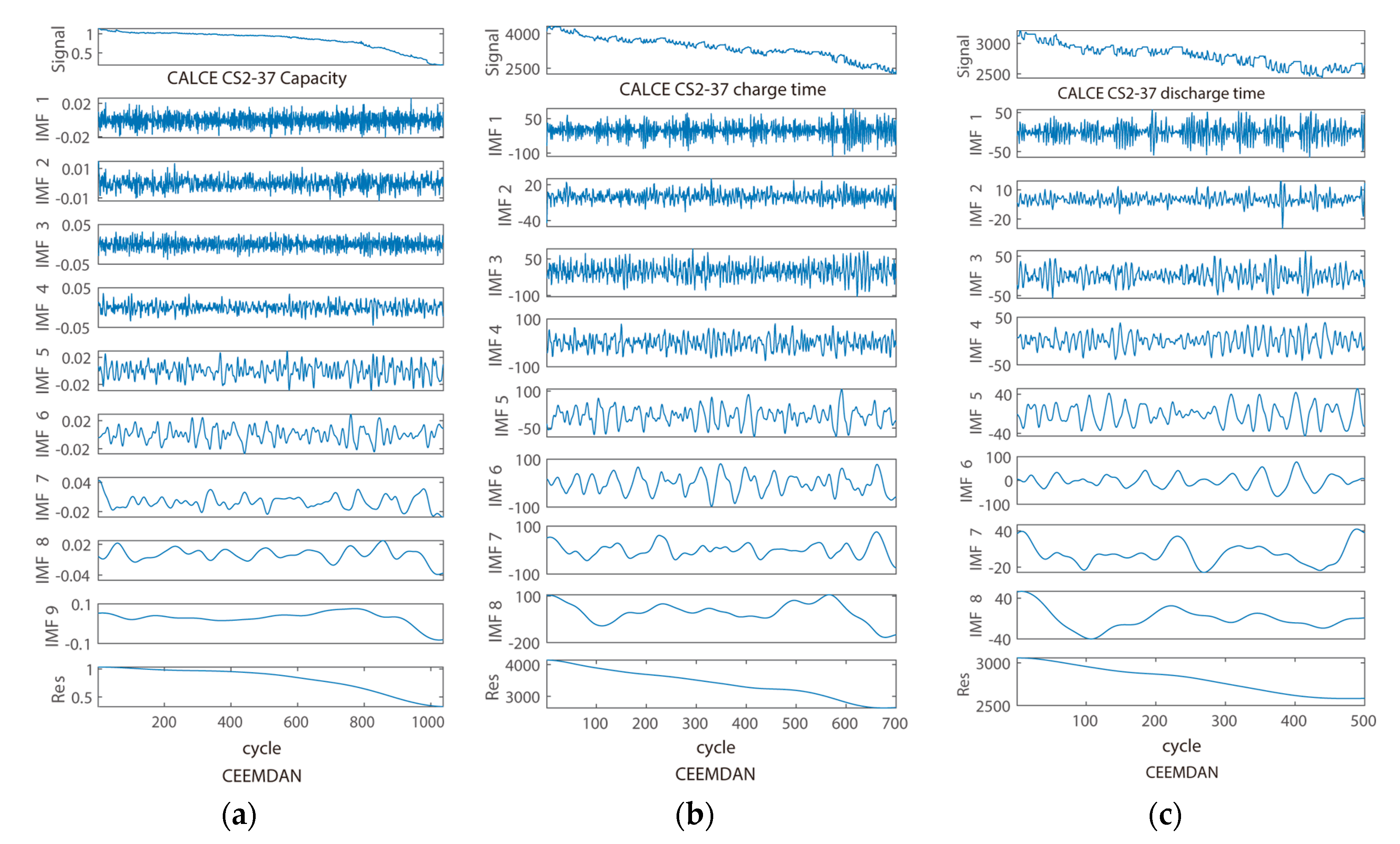
In practice, as the times of charging/discharging cycles increases, the data obtained by the sensor also increases. Here, choose different prediction starting points arbitrarily, that is, the known data in the experiment are different, also take CALCE CS2-37 as examples for analysis and research, use the above-mentioned signal decomposition algorithm [27,28,29,30,31,32] to decompose the battery health indicator time series data, the decomposition results are shown in Figure 3.

Figure 3a shows the capacity for all cycles, Figure 3b shows the charging time when it has been charged 700 cycles, and Figure 3c shows the discharge time with 500 cycles; the non-trend items (combination of other IMFs) are shown in Figure 4. It can be seen from the figures that the Health Indicators (capacity, time) extracted from the monitoring data obtained by sensors have been successfully decomposed into a set of modal functions (the Res in Figure 3 represents the residual term). Then, use Res as the basic trend, and the trend items are constructed using the reverse combination method, that is, first compare the Res with the original data, and if the difference is too big, the last IMF will be added to the basic Res. If this is not enough to describe the trend, the penultimate IMF will be added. After many experiments, usually, the Res or the combination of adding the last one or two IMFs can well represent the trend of the raw data. The steps to determine the trend items and non-trend items are as follows (take Figure 3a and Figure 4a as examples):

Step 1:

Assuming trend item = $Res$, non-trend item = ${\sum }_{i=1}^{9}IM{F}_i$

Step 2:

Determine whether the trend item is appropriate (such as mean calculation, correlation analysis, or other standards that are considered set, etc.)

Step 3:

If the trend item and trend item are inappropriate, assuming the trend term = $Res+IM{F}_9$, non-trend item = ${\sum }_{i=1}^{8}IM{F}_i$

Step 4:

Continue until the two items are suitable.

In this way, the raw data is divided into relatively smooth trend items and non-smooth trend items and then using the ARIMA and LSSVM to predict the two data series, respectively.

4. The ARIMA Model

4.1. Principle of the ARIMA Model

The ARIMA ($p,d,q$) model is an autoregressive integrated moving average model. This model transforms non-stationary time series into stationary time series, only the lag value of dependent variable, the present value and lag value of random error term are regressed. This is a commonly used random time series model. In the model, AR is an autoregressive model, MA is the moving average, d is the order of difference. The model converts non-stationary time series into stationary by D-order difference. The highest order of autocorrelation is $p$, and the highest order of moving average is $q$, this usually contains $p+q$ independent unknown coefficients. Since this is a common set of time series forecasting methods, only the necessary definitions and explanations will be made here, and no detailed description will be given [33,34,35,36].

Definition 1.

AR$\left(1\right)$, AR$\left(2\right)$and AR$\left(p\right)$model:

$$\{\begin{array}{l}AR\left(1\right)model:X_t=a_0+a_1{X}_{t-1}+{\epsilon }_t\hfill \\ AR\left(2\right)model:X_t=a_0+a_1{X}_{t-1}+a_2{X}_{t-2}+{\epsilon }_t\hfill \\ AR\left(p\right)model:X_t=a_0+a_1{X}_{t-1}+a_2{X}_{t-2}+\cdots +a_p{X}_{t-p}+{\epsilon }_t=a_0+{{\displaystyle \sum }}_{i=1}^p{a}_i{X}_{t-i}+{\epsilon }_t\hfill \end{array}$$

(6)

where${\epsilon }_t$is the white noise series, and$a_0,a_1,a_2,\cdots a_p$is$p+1$real numbers. This model is called the$p$-order autoregressive model, denoted as the AR$\left(p\right)$model, and the series$X_t$suitable for this model is called the AR ($p$) series.

Definition 2.

MA$\left(1\right)$, MA$\left(2\right)$and MA$\left(q\right)$model:

$$\{\begin{array}{l}MA\left(1\right)model:X_t=c_0+{\epsilon }_t-b_1{\epsilon }_{t-1}\hfill \\ MA\left(2\right)model:X_t=c_0+{\epsilon }_t-b_1{\epsilon }_{t-1}-b_2{\epsilon }_2\hfill \\ MA\left(q\right)model:X_t=c_0+{\epsilon }_t-b_1{\epsilon }_{t-1}-b_2{\epsilon }_2-\cdots -b_q{\epsilon }_q=c_0+{\epsilon }_t-{{\displaystyle \sum }}_{i=1}^q{b}_i{\epsilon }_{t-i}\hfill \end{array}$$

(7)

where$c_0$is a constant and${\epsilon }_t$is a white noise series.

Definition 3.

ARMA ($p,q$) model:

The ARMA ($p,q$) model is a combination of the AR ($p$) model and MA ($q$) model, which is an autoregressive moving average model, as shown in the equation below.

$$ARMA\left(p,q\right) model: X_t=a_0+{{\displaystyle \sum }}_{i=1}^p{a}_i{X}_{t-i}+{\epsilon }_t+{{\displaystyle \sum }}_{i=1}^q{b}_i{\epsilon }_{t-i\bullet }$$

(8)

where${\epsilon }_t$is a white noise sequence,${\forall }_s<t, E{X}_s{\epsilon }_t=0$If$a_0=0$, it is called decentralized ARMA ($p,q$) model.

If$q=0$, the model is AR ($p$).

If$p=0$, the model is MA ($q$).

Definition 4.

ARIMA (p,d,q) model:

The ARIMA ($p,d,q$) model first transforms the non-stationary historical data sequence$Y_t$into a stationary data sequence$X_t$by d-order difference processing, then establish an ARMA ($p,q$) model and predict, and finally restore the$d$-order difference to get the predicted data of$Y_t$.

After the ARIMA model is established, the characteristics of the autocorrelation function (ACF), partial autocorrelation function (PACF), as well as the Akaike Information Criterion (AIC) and Bayesian Information Criterion (BIC) are used to determine the order. After the model test, the prediction can be carried out. The prediction process of the trend items data series of SOH for lithium batteries based on the ARIMA model shows in Figure 5.

4.2. ARIMA Prediction Experiment of Trend Terms

As the battery gradually deteriorates, its dischargeable capacity will gradually decrease, and the chargeable/dischargeable time will also become shorter. Assuming that part of the battery data (300 cycles) has been monitored, the experimental results (CS2-37) is shown in Figure 6. Figure 6a is the capacity trend item decomposed by CEEMDAN, Figure 6b is the trend item prediction using ARIMA, and Figure 6c is the non-trend item after decomposition.

In Figure 6b, the ARIMA prediction model is based on Figure 6a. The red curve is the MMSE prediction result curve based on the ARIMA model. The thin gray dotted line is the multiple Monte Carlo simulation based on the ARIMA model. The blue curve is the mean value of multiple ARIMA Monte Carlo simulations. As can be seen in the figure, the results of the ARIMA multiple Monte Carlo simulation predictions are generally similar (multiple gray dotted lines). Besides, as the number of ARIMA Monte Carlo simulations increases (approximately hundreds of times), its average value is very close to the ARIMA MMSE prediction.

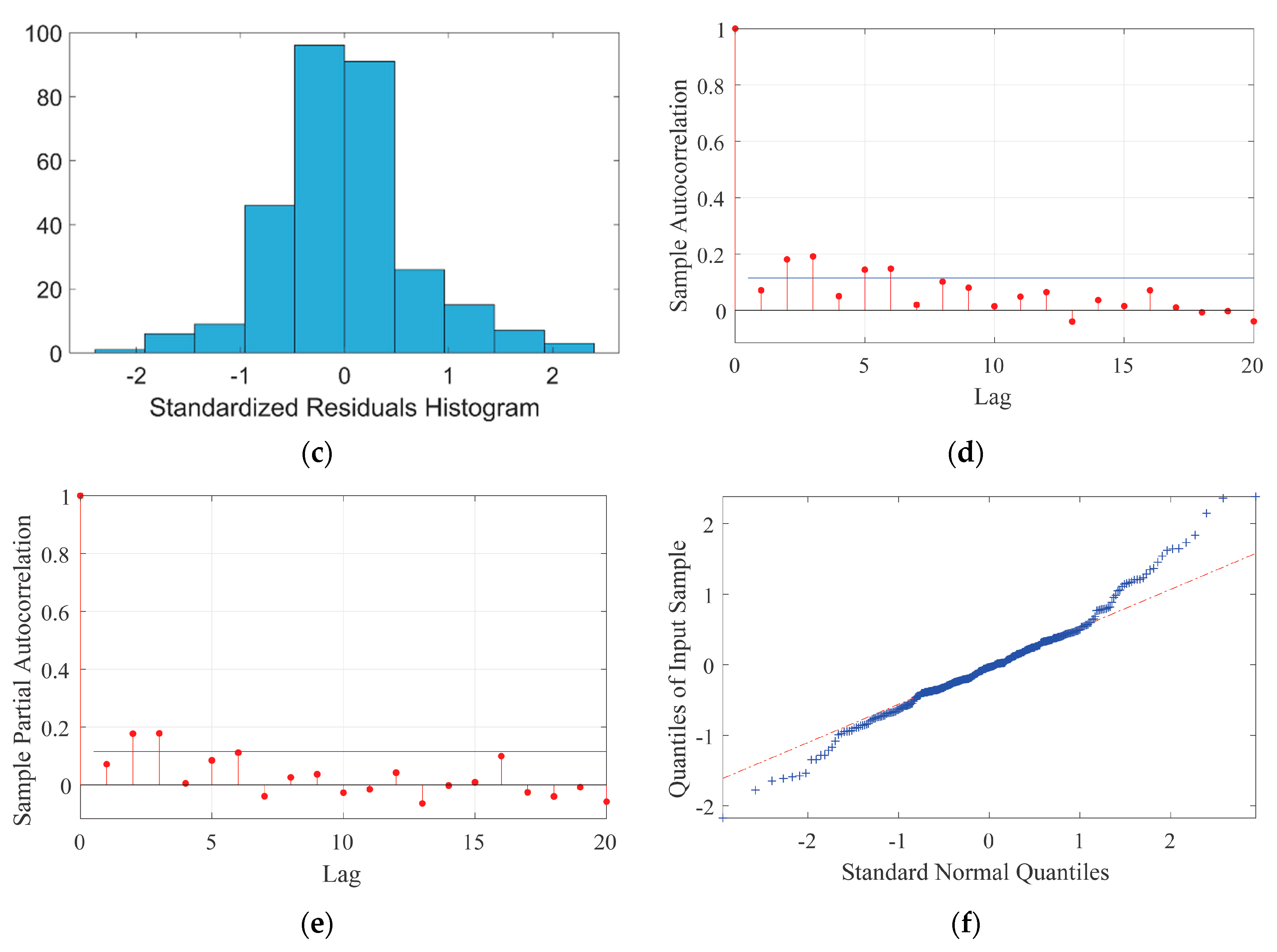
Figure 7 shows the residuals of ARIMA and results of residual testing (corresponding to Figure 6). Among the figures, QQplot is the relationship between the sample quantile and the theoretical quantile of the normal distribution. The QQplot in Figure 7 approximates a straight line, which means that it approximates the behavior of a normal distribution. So according to the statistical knowledge and the basic principles of ARIMA, and from the Figures of the autocorrelation function, partial autocorrelation function, and the QQPlot, it can be seen that the residual of this example contains less battery degradation information, so it can be decided whether to discard the residual according to the accuracy requirements. It can be seen from the above analysis that when the full-life reference model cannot be obtained in advance, the ARIMA model can predict the State of Health of the battery based on the part of the data that has been obtained. With the increase of monitoring data, the effect has gradually improved. However, there are certain errors in the current model and prediction results, and the correction of these errors will be corrected later.

4.3. Residuals of Autoregressive Integrated Moving Average Model

Generally, the residuals predicted by ARIMA should pass the autocorrelation test of 0.05 significance level (related to actual accuracy requirements). But, according to the actual situation and accuracy requirements, the residuals of the ARIMA model and the non-trend items obtained by CEEMDAN decomposition can be combined to construct new non-trend items, like the Figure 8b in Section 5.2 in this paper.

5. Prediction Based on LSSVM

5.1. Phase Space Reconstruction Theory

The support vector machine (SVM) is a regression method based on the VC dimension and structural risk minimization. It is suitable for nonlinear small sample problems. Least squares support vector machine (LSSVM) transforms the problem into solving linear equations and the convergence speed is faster [37,38,39,40,41,42]. Next, a brief description of its principle follows.

Suppose the input training data is

$$\left\{\left(x_1,y_1\right)\left(x_2,y_2\right)\cdots \left(x_l,y_l\right)\right\}$$

(9)

If $x$ is the nonlinear mapping, w is the weight coefficient of the feature space, and b is the offset, then the linear Equation (10) of the high-dimensional feature space can be used to fit the training data.

$$f\left(x\right)=w^T\phi \left(x\right)+b$$

(10)

According to the principle of structural risk minimization, LSSVM regression can be expressed as the constrained optimization problem of Equation (11):

$$\{\begin{array}{c}min \frac{1}{2}{w}^{T}w+\frac{\lambda }{2}{{\displaystyle \sum }}_{i=1}^l{e}_i^2\\ s.t. y_i=w^T\varphi \left(x_i\right)+b+e_i, i=1 ~ l\end{array}$$

(11)

Then the Lagrange function is introduced to transform the optimization problem of (11) to the dual space, and Equation (12) can be obtained:

$$L=\frac{1}{2}{w}^{T}w+\frac{\lambda }{2}{{\displaystyle \sum }}_{i=1}^l{e}_i^2-{{\displaystyle \sum }}_{i=1}^l{\alpha }_i\left(w^T\varphi \left(x_i\right)+b+e_i-y_i\right).$$

(12)

In Equation (12), $\alpha$ is the Lagrange multiplier and $\lambda$ is a constant. According to the Karush–Kuhn–Tucker (KKT) conditions, Equation (13) can be obtained:

$$\{\begin{array}{c}\partial L/\partial w=0\\ \partial L/\partial b=0\\ \partial L/\partial e_i=0\\ \partial L/\partial {\alpha }_i=0\end{array} \to \{\begin{array}{c}w={{\displaystyle \sum }}_{i=1}^l{\alpha }_i\varphi \left(x_i\right)\\ {{\displaystyle \sum }}_{i=1}^l{\alpha }_i=0\\ {\alpha }_i=\gamma e_i\\ w^T\varphi \left(x_i\right)+b+e_i-y_i=0\end{array}$$

(13)

According to Equation (13), Equation (14) can be obtained:

$$\{\begin{array}{c}\left[\begin{array}{cc}0& e_l^T\\ e_l& Q+I/\gamma \end{array}\right]\left[\begin{array}{c}b\\ \alpha \end{array}\right]=\left[\begin{array}{c}0\\ y\end{array}\right]\\ \{\begin{array}{c}{e}_l={(1, 2, \cdots l)}^T\\ \alpha ={({\alpha }_1, {\alpha }_l)}^T\\ y={(y_1, y_l)}^T\\ Q=\varphi {\left(x_i\right)}^T\varphi \left(x_i\right)\end{array}\end{array}$$

(14)

According to the Mercer condition, Equation (15) can be obtained:

$$\{\begin{array}{c}k\left(x_i,x_j\right)=\varphi {(x_i)}^T\varphi \left(x_i\right)\\ f\left(x\right)={{\displaystyle \sum }}_{i=1}^l{\alpha }_{i}k\left(x_i,x_j\right)+b\end{array}$$

(15)

In Equation (14), $\gamma$ is also the model parameter. In this paper, the multi-dimensional input 1-dimensional output predictor is constructed; for example, the input of 5-dimensional predictor can be expressed as Equation (16).

$$\left\{x_2, \cdots x_{m+1}; x_2,\cdots x_{m+1}; x_3,\cdots x_{m+2}; x_4,\cdots x_{m+3}; x_5,\cdots x_{m+5}\right\}$$

(16)

To determine the LSSVM parameters, two methods are tested here. Cross-validation is to divide the data into training set and validation set, use the training set to train the model, use the validation set to test the model and conduct evaluation, and then solve the model parameters when the performance index of the model is the best. Another method is to use the particle swarm optimization (PSO) method. The steps of PSO are as follows,

Step 1:

Initialize, such as speed, position, inertia factor, acceleration constant, number of iterations cycles, etc.

Step 2:

Evaluate the initial fitness value of each particle and use it as the local optimal value of the particle, and its position as the location of the local optimal value of the particle.

Step 3:

Take the best initial adaptation value as the current global optimal value, and its position as the location of the global optimal value.

Step 4:

Update the flying speed of each particle according to Equation (17) and limit the amplitude, and update the current position of the particle. In the formula, $i=1\cdots m$, $d=12\cdots D$, $w$ is an inertia factor (non-negative number), $c1,c2$ is a non-negative constant acceleration factor, $r1,r2$ are random numbers in (0,1), $\alpha$ is the constraint factor used to control the speed weight, $m$ is the number of particles, $D$ is the dimension of the target search space.

$$\{\begin{array}{l}{v}_i^d=w{v}_i^d+c_1{r}_1\left(p_i^d-x_i^d\right)+c_2{r}_2\left(p_g^d-x_i^d\right)\hfill \\ x_i^d=x_i^d+\alpha v_i^d\hfill \end{array}$$

(17)

Step 5:

Compare the effect of the current particle fitness value. If satisfied, the current fitness value is regarded as the local optimum, and its position is regarded as the location of the particle’s local optimum.

Step 6:

Find the global optimal value in the current swarm and use it as the location of the global optimal value of the particle swarm.

Step 7:

Repeat steps 4–6 until the number of iterations is reached.

Step 8:

Output the global optimal value and position of the particle swarm, the local optimal value and the position of each particle.

5.2. Prediction Experiment of Non-Trend Data Sequence of Lithium Battery Health Indicator

Since the trend item can usually reflect the degradation trend of the battery. Comparing the prediction of the trend item with the original data we can observe the experimental effect. In fact, the results of modal decomposition have a certain relationship with the data, and the results of the modal decomposition of all data and partial data are not necessarily the same. When only part of the data is known in practical applications, it is inconvenient to directly compare the prediction effects. Therefore, the data of the entire life cycle is decomposed in the proposed scheme, and then part of the data of non-trend items is regarded as known, and experiments are carried out in this way to verify the effect of the experiment.

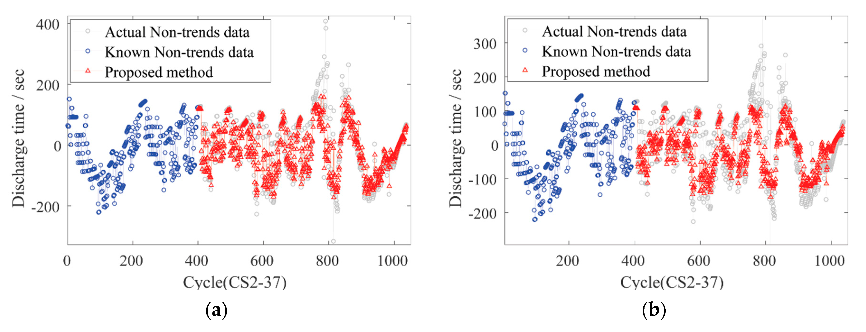
Next, we take the non-trend item data obtained from the full life cycle modal decomposition of CS2-37 as an example, and test two methods of LSSVM, direct prediction and recursive prediction. Figure 8a shows the CEEMDAN decomposition trend items and non-trend items for all data. Figure 8b is the LSSVM direct prediction of the non-trend items in proposed in scheme (CEEMDAN decomposition trend term and ARIMA residual combination as a new non-trend term). Figure 8c,d is another experiment (only the starting point is predicted to become the 700th cycle). Here, the two conclusions can be drawn from Figure 8. Firstly, the results of each CEEMDAN decomposition are not necessarily the same (such as Figure 8a,c are not exactly the same), but they basically reflect the deterioration trend of the battery. Secondly, ARIMA prediction of non-trend items may be seriously wrong but LSSVM will not. Besides, in the experiments later in this article, the residual error by ARIMA predicted is added to the non-trend item data decomposed by CEEMDAN to maintain the integrity of the data. Here, because the step size of direct prediction is limited by the known data length, the last short segment is a straight line.

Figure 9 shows the experimental results of the recursive prediction. Among them, Figure 9a is a 1-step recursive cross-validation LSSVM prediction with a prediction starting point of 400, Figure 9b is 3-step recursive cross-validation LSSVM prediction, and Figure 9c is 1-step recursive prediction of particle swarm optimization-least squares support vector machine (PSOLSSVM). Figure 9d is 1-step recursive cross-validation LSSVM prediction with a prediction starting point of 600, Figure 9e is 3-step recursive cross-validation LSSVM prediction, and Figure 9f is 3-step recursive prediction of PSOLSSVM. It can be seen from the figures that the short-term prediction of LSSVM with cross-validation optimization and PSO optimization has achieved relatively satisfactory results, but after many experiments, the following two conclusions have been obtained. First, the LSSVM recursive prediction gradually becomes worse as the prediction step size increases. Second, the speed of PSO optimization is slower than that of cross-validation.

As can be seen from the above experiment that, based on LSSVM, the non-trend items can be predicted within a certain period, but the long-term error is large, which is consistent with the principle of LSSVM prediction. Besides, the prediction results of non-trend items are generally within the range of known non-trend items, but there are serious errors in the prediction of non-trend projects based on ARIMA, and by adding the residual of ARIMA prediction to the non-trend items for processing, it is helpful to reduce the loss of information. Therefore, in the prediction of SOH of unknown types of lithium batteries, use of the ARIMA model predicts the general degradation trend of SOH in a certain period, and assisting the LSSVM prediction can improve the prediction effect. For details of the results of the comprehensive evaluation experiment of SOH, please refer to Section 6.

6. Comprehensive Evaluation of the SOH and Discussion

In this paper, experiments are carried out in three cases, and these experiments are used to verify the effectiveness of the proposed scheme. The first case is the use of Capacity Health Indicator, such as CS2-35 battery. The second case is the use of Charge Time Health Indicator, such as CS2-35, CS2-37. The third case is the use of Discharge Time Health Indicator, such as CS2-37, CS2-34.

6.1. Experimental Results

The 13 experimental results of the proposed method are as follows. Among them, the trend items are predicted by using ARIMA, and then the predicted residuals are combined with the non-trend items obtained by CEEMDAN decomposition to construct new non-trend items, and using LSSVM (cross-validation) to predict. Finally, the prediction results of the two are combined to evaluate the SOH of the lithium battery (the red triangle in the figure is the experimental result, the blue line is the number of cycles the battery has been used). It can be seen from the results that when the appropriate ARIMA parameters cannot be obtained, the scheme proposed can effectively improve the prediction effect (compared with the black curve).

6.2. Discuss

Figure 10 and Figure 11 are the experimental results of CS2-35 based on Capacity and Charge Time Health Indicators, respectively. As can be seen from Figure 10, the scheme proposed has a better prediction effect than ARIMA. In Figure 10a, the ARIMA method fails to predict the decline of the battery. The proposed scheme predicts the decline of the battery. In Figure 10b,c, the proposed scheme is corrected to some extent under the condition that ARIMA can predict the battery degradation. The results in Figure 11 are similar to Figure 10. In Figure 11a,b, the proposed scheme is better corrected than the results of the ARIMA scheme. The prediction deviation of ARIMA in Figure 11c is larger, and the prediction deviation of the proposed scheme is smaller.

Figure 12 shows the experimental results of CS2-37 battery based on the Discharge Time Health Indicator. From Figure 12a, it can be seen that because there is no full cycle life model of the same type of battery as a reference, and the amount of data is small; the effect of this experiment is not particularly perfect. However, compared with ARIMA, the proposed scheme still predicts fluctuations to a certain extent, and the ARIMA model does not predict the fluctuations well. After many experiments, it can be found that as the battery continues to be used, more and more data is obtained, and the prediction effect is significantly improved, such as shown in Figure 12b, the proposed scheme has improved a lot compared with ARIMA. In Figure 12c, the ARIMA model automatically constructed based on the AIC–BIC criterion has a wrong prediction, but the proposed scheme can continue to predict.

Figure 13 shows the experimental results of CS2-34 based on Discharge Time Health Indicator and CS2-37 based on Charge Time Health Indicator. It can also be seen from these figures that, in the case where the full-life data model cannot be obtained as a reference model, the scheme proposed can effectively evaluate the SOH of lithium batteries by relying on only part of the historical data. And when the monitored battery data changes significantly, the scheme proposed in this article can also continue to make a good prediction of the SOH of the batteries.

6.3. Error Analysis

In Section 6.1, Figure 10d is the error analysis of the three predictions in Figure 10. Figure 10d is also the error analysis of the three predictions in Figure 11. Figure 12d is the error analysis of the three predictions in Figure 12. Figure 13c,f is the error analysis of the three predictions in Figure 13.

In Figure 10d, the error of the three prediction experiments using the proposed scheme (CEEMDAN-ARIMA-LSSVM) is better than that of the direct prediction scheme without decomposition. In Figure 11d, the error of two experiments has been improved (corresponding to Figure 11a,b, and the error of one experiment has been greatly improved (corresponding to Figure 11c). In Figure 12d, the short-term error of the first experiment was improved, and the long-term prediction error was not significantly different from the direct prediction scheme without decomposition (corresponding to Figure 12a). The error of the second experiment is also effectively improved (Figure 12b). In the third experiment, the proposed scheme avoids false prediction of the scheme without decomposition (Figure 12c). Here, since the health status of the battery is getting worse and worse as a whole, but the prediction in Figure 12c is not the case, we define this prediction as a false prediction.

As can be seen from Figure 13a–c, the two experimental results with direct prediction without prior decomposition had a false prediction, but the proposed scheme avoids this false phenomenon. The error of the first experiment has been improved, the short-term effect of the second experiment is better, and the long-term prediction effect is not as good as the short-term prediction. It can be seen from Figure 13f that the error of the second experiment has been effectively improved (corresponding to Figure 13d). In the first experiment, the medium and short-term (before about 800 cycles) prediction distortion is effectively improved (Figure 13e). However, the effect of long-term prediction (after about 800 cycles) is not as good as that of medium and short term prediction.

From the above experiments, it can be found that when the data monitored by the battery suddenly change significantly. For example, the capacity of the battery or the charging/discharging time suddenly drops rapidly due to some reasons at some time or the short-term energy regeneration phenomenon caused by the battery’s short rest. In this case, using the scheme proposed in this article for forecasting can better improve the forecasting effect. Besides, if the short-term prediction of SOH of the battery is needed, LSSVM-based recursive prediction can be considered to predict non-trend items according to demand. The experimental process is similar to this, except that the prediction results of non-trend items are slightly different, similar to the results shown in Figure 9, and because when only the known data is decomposed, the decomposition result of the new non-trend item cannot be known in advance, but Figure 9 can be used instead of verification. It can be seen from the figure that the experimental effects of non-trend projects can achieve the expected results relatively well.

7. Conclusions

Generally, the SOH prediction of lithium batteries mainly relies on degradation data of the same type of batteries to construct a reference model, and calculates the discharge capacity of the batteries in the historical cycle to estimate their future available capacity. However, when the reference model based on the full-life data of the same type of battery cannot be obtained in advance, it is more difficult to predict its SOH. Besides, the degradation of the battery involves very complicated internal chemical and material factors, etc. So this is a non-linear and uneven degradation process, and it is not possible to obtain the required accurate battery life degradation model in every situations, various reasons make the application of online prediction more difficult.

In this paper, a data series based on the capacity and charge/discharge time was extracted from the lithium battery data set, their correlations analyzed, constructed as a Health Indicator of the batteries, and then the known Health Indicator data series is decomposed using the CEEMDAN algorithm. Then, select the appropriate IMFs to construct the trend item of the Health Indicator according to the demand (reverse order combination), and use the ARIMA model to predict it. Next, combine the ARIMA prediction residual with the remaining IMFs to construct a new non-trend item, and use the LSSVM method to predict the newly constructed non-trend items (use cross-validation or PSO to find the optimal parameters as required). Finally, the prediction results of the two are combined to make a comprehensive assessment of the SOH of lithium batteries.

In the experimental part of Section 6, by using the proposed scheme, and taking the capacity, charging time and discharge time as Health Indicators, the three batteries (CS2-35, CS2-34, CS2-37) were tested. The experimental results are given in Section 6.1, and these results are discussed in Section 6.2. These experimental results verify the effectiveness of the proposed scheme. Besides, the scheme can also effectively improve the prediction effect when the data monitored by the battery changes greatly, such as when the data suddenly drops or when the energy regeneration causes the data to rise suddenly. In addition, the solution proposed in this paper only relies on partial historical data, therefore, it can be used in a wider range of applications, such as in the case of unknown battery type, that is to say, when it is difficult to establish a full-life model based on the degradation data of the same type of battery, and this scheme can predict the SOH of the battery online.

References

1. Saha, B.; Goebel, K.; Poll, S.; Christophersen, J. Prognostics Methods for Battery Health Monitoring Using a Bayesian Framework. IEEE Trans. Instrum. Meas. 2009, 58, 291–296. [Google Scholar] [CrossRef]
2. Saha, B.; Goebel, K.; Christophersen, J. Comparison of Prognostic Algorithms for Estimating Remaining Useful Life of Batteries. Trans. Inst. Meas. Control 2009, 31, 293–308. [Google Scholar] [CrossRef]
3. He, W.; Williard, N.; Osterman, M.; Pecht, M. Prognostics of Lithium-Ion Batteries Based on Dempster-Shafer Theory and the Bayesian Monte Carlo Method. J. Power Sources 2011, 196, 10314–10321. [Google Scholar] [CrossRef]
4. Wang, D.; Miao, Q.; Pecht, M. Prognostics of Lithium-Ion Batteries Based on Relevance Vectors and a Conditional Three-Parameter Capacity Degradation Model. J. Power Sources 2013, 239, 253–264. [Google Scholar] [CrossRef]
5. Xing, Y.; Ma, E.W.M.; Tsui, K.L.; Pecht, M. An Ensemble Model for Predicting the Remaining Useful Performance of Lithium-Ion Batteries. Microelectron. Reliab. 2013, 53, 811–820. [Google Scholar] [CrossRef]
6. Liu, D.; Wang, H.; Peng, Y.; Xie, W.; Liao, H. Satellite Lithium-Ion Battery Remaining Cycle Life Prediction with Novel Indirect Health Indicator Extraction. Energies 2013, 6, 3654–3688. [Google Scholar] [CrossRef]
7. Liu, D.; Zhou, J.; Liao, H.; Peng, Y.; Peng, X. A Health Indicator Extraction and Optimization Framework for Lithium-Ion Battery Degradation Modeling and Prognostics. IEEE Trans. Syst. Man Cybern. Syst. 2015, 64, 660–670. [Google Scholar] [CrossRef]
8. Liu, D.; Xie, W.; Liao, H.; Peng, Y. An Integrated Probabilistic Approach to Lithium-Ion Battery Remaining Useful Life Estimation. IEEE Trans. Instrum. Meas. 2015, 45, 915–928. [Google Scholar] [CrossRef]
9. Zhou, Y.; Huang, M.; Chen, Y.; Tao, Y. A Novel Health Indicator for On-Line Lithium-Ion Batteries Remaining Useful Life Prediction. J. Power Sources 2016, 321, 1–10. [Google Scholar] [CrossRef]
10. Huang, S.-C.; Tseng, K.-H.; Liang, J.-W.; Chang, C.-L.; Pecht, M.G. An Online SOC and SOH Estimation Model for Lithium-Ion Batteries. Energies 2017, 10, 512. [Google Scholar] [CrossRef]
11. Su, X.; Wang, S.; Pecht, M.; Zhao, L.; Ye, Z. Interacting Multiple Model Particle Filter for Prognostics of Lithium-Ion Batteries. Microelectron. Reliab. 2017, 70, 59–69. [Google Scholar] [CrossRef]
12. Ren, L.; Zhao, L.; Hong, S.; Zhao, S.; Wang, H.; Zhang, L. Remaining Useful Life Prediction for Lithium-Ion Battery: A Deep Learning Approach. IEEE Access 2018, 6, 50587–50598. [Google Scholar] [CrossRef]
13. Sun, Y.; Hao, X.; Pecht, M.; Zhou, Y. Remaining Useful Life Prediction for Lithium-Ion Batteries Based on an Integrated Health Indicator. Microelectron. Reliab. 2018, 88–90, 1189–1194. [Google Scholar] [CrossRef]
14. Wei, J.; Dong, G.; Chen, Z. Remaining Useful Life Prediction and State of Health Diagnosis for Lithium-Ion Batteries Using Particle Filter and Support Vector Regression. IEEE Trans. Ind. Electron. 2018, 65, 5634–5643. [Google Scholar] [CrossRef]
15. Zhang, L.; Mu, Z.; Sun, C. Remaining Useful Life Prediction for Lithium-Ion Batteries Based on Exponential Model and Particle Filter. IEEE Access 2018, 6, 17729–17740. [Google Scholar] [CrossRef]
16. Zhang, Y.; Xiong, R.; He, H.; Pecht, M.G. Lithium-Ion Battery Remaining Useful Life Prediction with Box-Cox Transformation and Monte Carlo Simulation. IEEE Trans. Ind. Electron. 2019, 66, 1585–1597. [Google Scholar] [CrossRef]
17. Jia, J.; Liang, J.; Shi, Y.; Wen, J.; Pang, X.; Zeng, J. SOH and RUL Prediction of Lithium-Ion Batteries Based on Gaussian Process Regression with Indirect Health Indicators. Energies 2020, 13, 375. [Google Scholar]
18. Zhou, Y.; Huang, M. Lithium-Ion Batteries Remaining Useful Life Prediction Based on a Mixture of Empirical Mode Decomposition and ARIMA Model. Microelectron. Reliab. 2016, 65, 265–273. [Google Scholar] [CrossRef]
19. Chen, L.; Xu, L.; Zhou, Y. Novel Approach for Lithium-Ion Battery On-Line Remaining Useful Life Prediction Based on Permutation Entropy. Energies 2018, 11, 820. [Google Scholar] [CrossRef] [Green Version]
20. Mao, L.; Xu, J.; Chen, J.; Zhao, J.; Wu, Y.; Yao, F. A LSTM-STW and GS-LM Fusion Method for Lithium-Ion Battery Rul Prediction Based on EEMD. Energies 2020, 13, 2380. [Google Scholar] [CrossRef]
21. Yun, Z.; Qin, W. Remaining Useful Life Estimation of Lithium-Ion Batteries Based on Optimal Time Series Health Indicator. IEEE Access 2020, 8, 55447–55461. [Google Scholar] [CrossRef]
22. CALCE Battery Research Group of the University of Maryland. Battery Data Set. Available online: https://web.calce.umd.edu/batteries/data.htm (accessed on 12 September 2020).
23. Gibbons, J.D.; Chakraborti, S. Nonparametric Statistical Inference, 5th ed.; CRC Press, Taylor & Francis Group: New York, NY, USA, 2011; pp. 389–416. [Google Scholar]
24. Puth, M.; Neuh, M. Effective Use of Pearson’s Product-Moment Correlation Coefficient. Anim. Behav. 2014, 93, 183–189. [Google Scholar] [CrossRef]
25. Cheng, J.; Yu, D.; Yang, Y. Application of Support Vector Regression Machines to the Processing of end Effects of Hilbert-Huang Transform. Mech. Syst. Signal Process. 2007, 21, 1197–1211. [Google Scholar] [CrossRef]
26. El Bouny, L.; Khalil, M.; Adib, A. ECG Signal Filtering Based on CEEMDAN with Hybrid Interval Thresholding and Higher Order Statistics to Select Relevant Modes. Multimed. Tools Appl. 2019, 78, 13067–13089. [Google Scholar] [CrossRef]
27. Rezaie-Balf, M.; Maleki, N.; Kim, S.; Ashrafian, A.; Babaie-Miri, F.; Kim, N.W.; Chung, I.-M.; Alaghmand, S. Forecasting Daily Solar Radiation Using CEEMDAN Decomposition-Based MARS Model Trained by Crow Search Algorithm. Energies 2019, 12, 1416. [Google Scholar] [CrossRef] [Green Version]
28. Li, T.; Zhou, Y.; Li, X.; Wu, J.; He, T. Forecasting Daily Crude Oil Prices Using Improved CEEMDAN and Ridge Regression-Based Predictors. Energies 2019, 12, 3603. [Google Scholar] [CrossRef] [Green Version]
29. Flandrin, P.; Torres, E.; Colominas, M.A. A Complete Ensemble Empirical Mode Decomposition with Adaptive Noise. In Proceeding of the 2011 IEEE International Conference on Acoustics, Speech and Signal Processing (ICASSP), Prague, Czech Republic, 22–27 May 2011; pp. 4144–4147. [Google Scholar]
30. Chaabi, L.; Lemzadmi, A.; Djebala, A.; Bouhalais, M.L.; Ouelaa, N. Fault Diagnosis of Rolling Bearings in Non-Stationary Running Conditions Using Improved CEEMDAN and Multivariate Denoising Based on Wavelet and Principal Component Analyses. J. Adv. Manuf. Technol. 2020, 107, 3859–3873. [Google Scholar] [CrossRef]
31. Li, G.; Yang, Z.; Yang, H. A Denoising Method of Ship Radiated Noise Signal Based on Modified CEEMDAN, Dispersion Entropy, and Interval Thresholding. Electron. 2019, 8, 597. [Google Scholar] [CrossRef] [Green Version]
32. Mousavi, A.A.; Zhang, C.; Masri, S.F.; Gholipour, G. Structural Damage Localization and Quantification Based on a CEEMDAN Hilbert Transform Neural Network Approach: A Model Steel Truss Bridge Case Study. Sensors 2020, 20, 1271. [Google Scholar] [CrossRef] [Green Version]
33. Wang, J.; Hu, J. A Robust Combination Approach for Short-Term Wind Speed Forecasting and Analysis—Combination of the ARIMA (Autoregressive Integrated Moving Average), ELM (Extreme Learning Machine), SVM (Support Vector Machine) and LSSVM (Least Square SVM) Forecasts Using a GPR (Gaussian Process Regression) Model. Energy 2015, 93, 41–56. [Google Scholar] [CrossRef]
34. Yuan, C.; Liu, S.; Fang, Z. Comparison of China’s Primary Energy Consumption Forecasting by Using ARIMA (the Autoregressive Integrated Moving Average) Model and GM(1,1) Model. Energy 2016, 100, 384–390. [Google Scholar] [CrossRef]
35. Singh, S.N.; Mohapatra, A. Repeated Wavelet Transform Based ARIMA Model for Very Short-Term Wind Speed Forecasting. Renew. Energy 2019, 136, 758–768. [Google Scholar] [CrossRef]
36. Ordóñez, C.; Sánchez Lasheras, F.; Roca-Pardiñas, J.; de Cos Juez, F.J. A Hybrid ARIMA–SVM Model for the Study of the Remaining Useful Life of Aircraft Engines. J. Comput. Appl. Math. 2019, 346, 184–191. [Google Scholar] [CrossRef]
37. Chen, Z.; Xue, Q.; Liu, Y.; Shen, J.; Xiao, R. State of Health Estimation for Lithium-Ion Batteries Based on Elman Neural Network. Renew. IEEE Access 2019, 7, 102662–102678. [Google Scholar] [CrossRef]
38. Pan, Y.; Hong, R.; Chen, J.; Singh, J.; Jia, X. Performance Degradation Assessment of a Wind Turbine Gearbox Based on Multi-Sensor Data Fusion. Mech. Mach. Theory 2019, 137, 509–526. [Google Scholar] [CrossRef]
39. Wang, Y.; Ni, Y.; Li, N.; Lu, S.; Zhang, S.; Feng, Z.; Wang, J. A Method Based on Improved Ant Lion Optimization and Support Vector Regression for Remaining Useful Life Estimation of Lithium-Ion Batteries. Energy Sci. Eng. 2019, 7, 2797–2813. [Google Scholar] [CrossRef]
40. Cheng, Y.; Zerhouni, N.; Lu, C. A Hybrid Remaining Useful Life Prognostic Method for Proton Exchange Membrane Fuel Cell. Energy Sci. Eng. 2018, 43, 12314–12327. [Google Scholar] [CrossRef]
41. Xue, X. Prediction of Slope Stability Based on Hybrid PSO and LSSVM. J. Comput. Civ. Eng. 2016, 31, 04016041. [Google Scholar] [CrossRef]
42. Long, B.; Xian, W.; Li, M.; Wang, H. Improved Diagnostics for the Incipient Faults in Analog Circuits Using LSSVM Based on PSO Algorithm with Mahalanobis Distance. Neurocomputing 2014, 133, 237–248. [Google Scholar] [CrossRef]
Figure 1. The capacity, charge time, and discharge time curve (CS2-37 battery): (a) capacity; (b) charge time and capacity; (c) discharge time and capacity.
Energies 13 04858 g001
Figure 2. Flowchart of the proposed experiment scheme.
Energies 13 04858 g002
Figure 3. Decompose by using CEEMDAN (CS2-37): (a) capacity; (b) charge time; (c) discharge time.
Energies 13 04858 g003
Figure 4. Non-trend items (all Intrinsic Mode Functions except the residuals) of the decomposition by using EMD, EEMD, and CEEMDAN (CS2-37): (a) capacity (corresponding Figure 3a); (b) charge time (corresponding Figure 3b); (c) discharge time (corresponding Figure 3c).
Energies 13 04858 g004
Figure 5. Flowchart of the ARIMA model prediction.
Energies 13 04858 g005
Figure 6. CEEMDAN decomposition and prediction of trend items (CS2-37): (a) trend items obtained by CEEMDAN; (b) trend items predicted based on ARIMA; (c) CEEMDAN non-trend items.
Energies 13 04858 g006
Figure 7. Residual and residual test (CS2-37): (a) residuals; (b) standardized residuals; (c) standardized residuals histogram; (d) autocorrelation function; (e) partial autocorrelation function; (f) QQ plot.
Energies 13 04858 g007aEnergies 13 04858 g007b
Figure 8. Experimental results (CEEMDAN discharging time of the CS2-37 battery).
Energies 13 04858 g008
Figure 9. Experimental results (CEEMDAN discharging time of the CS2-37 battery): (a,b,d,e) cross-validation least square support vector machine (LSSVM); (c,f) PSOLSSVM.
Energies 13 04858 g009aEnergies 13 04858 g009b
Figure 10. Experimental results (capacity of the CS2-35 battery).
Energies 13 04858 g010
Figure 11. Experimental results (charging time of the CS2-35 battery).
Energies 13 04858 g011aEnergies 13 04858 g011b
Figure 12. Experimental results (discharging time of the CS2-37 battery).
Energies 13 04858 g012
Figure 13. Experimental results (discharging time of CS2-34/charging time of CS2-37).
Energies 13 04858 g013