Abstract
Future power systems will be based on the more active role of distribution system and its cooperation with transmission system. The main issue, which will appear in the network, is the congestion. Congestion management will become one of the crucial elements of power system operation since Distributed Energy Resources (DERs) will be playing a more important role in power systems. Moreover, the evolution also changed the character of the systems to be more dynamic—the need for precise description of power flow and shares of particular nodes in line flows will emerge. This paper presents the potential solution to the congestion management problem by using the active role of the distribution system, which may dismantle the congestions by offering flexibility services. The tools which will be indispensable in this process will be Power Flow Tracing (PFT) methods. The main goal of this paper is to present modification of PFT method and its possible applications. The correctness of the Modified Inage Domain (MID) method is verified. The identification, verification and possible applications of the new MID method are also shown in the paper. It has been proven that the new method may be used in applications of allocation of transmission cost and in application in modern power systems for advanced congestion management.
1. Introduction
The development of the electricity sector, especially Renewable Energy Sources (RES) and DERs, is partially caused by the European legislative packages, which are setting valuable targets in different areas such as the European Union (EU) target of 32% of renewable energy in 2030 [1]. Moreover, investments in the sector are growing in popularity, due to its profitability and positive impact on society. Along with a gradual increase in capacity of RES and its intermittency, the network has become more congested in the transmission and distribution network. Despite the current changes, the congestions existed previously within the network; however, their nature and the origins were different, due to stable generation schemes and substantial load profiles.
Nowadays the congestions appear temporally rather than continuously and they are mostly caused by RESs or DERs. What is more, congestions happen more unexpectedly and there is a problem with limiting them in order to optimize operational conditions for power system. Moreover, since the amount of power produced in RESs and DERs is growing, the power system is losing controllable sources such as thermal power plants. In fact, in the grids based on Alternating Current (AC) there is no means to control the power, besides control of power sources (conventional power plants and RES) or possibility to reconfigure the network. However, RES and conventional power plants are controllable in different manners, in case of large power plants operator may reduce or increase produced power within technical constraints; in case of RES operator may only reduce produced power, since the source is producing power from available primary energy. Due to decreasing capacity of controllable sources, a need to introduce another systems may appear. In the Direct Current (DC) networks or in DC connections between the AC grids, control of the power is realized by DC terminals.
Alongside the growth of generation from renewable sources, the future grid will have to be either interconnected by DC connections or will have to have dynamic responses from smaller generations or loads located in the distribution sector. It will require a significant amount of capacity installed to satisfy the need for power with large amounts of curtailment. The power system has to have the ability to follow the fluctuations of base demand and variable generation from RES, so as to reassure the balance of the power in the grid. What is more, nowadays there is no active cooperation in congestion management between Transmission System Operator (TSO) and Distribution System Operator (DSO), whereas the active role of the distribution system will be crucial in the near future. Nowadays most of the Low Voltage (LV) and even Medium Voltage (MV) distribution grid is not being metered smartly; they are oversized to the parameters, which normally are not reached in peak of demand (since frequently peaks for demands are not reached in the same time). It will not be the case in the example for photovoltaic (PV) located in small area (connected to the same distribution line) and that is why currently the congestions mostly do not happen in the distribution network. However, with the growth of RES in distribution networks, there is an additional risk that congestion will start to occur also in the distribution grid and it is needed to prepare strong actions to prevent it. One of the solutions is an introduction of flexibility of resources in the distribution grid [2,3]. However, for now the congestion in distribution grid is out of the scope of this research.
The most important action in accordance with creating an active role of the distribution system is to increase the usage of renewable sources for services, along with an increase in the ability to control the power injected to the network. One of possible results of such action is that RES potentially may have a share in dismantling the congestion. The flexibility services of the distribution system can have a great impact on the system balancing, reducing the congestion and integrating renewable sources [4]. The framework of the prospective TSO–DSO cooperation is studied nowadays; the result of the work can be found in [5].
The insights of the discussed area may be found in the following literature review, where the core of the paper is discussed in detail on the basis of cited publications. Among others, discussed are aspects such as: congestion in transmission system, Power Transfer Distribution Factors (PTDF) and PFT.
2. Literature Review
The literature review will contain all of the aspects which will be further used in method identification, verification and presentation of potential applications.
2.1. Congestion in Transmission System
Congestion in transmission system occurs when the power flowing in line reaches operational limits, in case of some operators temporal overloads up to 20% are allowed. It is connected without fulfilling the established plan of energy delivery in the system or alternatively with emergency conditions. It may lead to the system instability, loss of the element of the network, if the security constraints are not satisfied. However, the international grid codes do not fully define the limits of congestions [3].
The methods of dismantling the congestion can be either classified as short term or long term solutions. Nowadays one of the most common ways to dismantle the congestion in the transmission network, classified as a short term solution, is the redispatch. It has an impact on the generation units—the unit, which produces electricity with the lower cost has to be substituted by the unit with the higher production cost. It influences the energy price and additionally the generation units working in the base load are not flexible enough to follow the change in the grid, which happens more rapidly. Another method of dismantling the congestion can be generation curtailment, which can be mainly associated with RES. Another short term solution of congestion dismantling is switching off the components of the power system (the ones that may be overloaded, to modify power flow), changing the position of taps in transformers or changing the configuration of the network. The common measure applied by some countries is reconfiguration of the system—in case of danger of system stability, there is a possibility to turn off the potentially overloaded lines [6,7,8].
The other methods classified as long term are connected with the expansion of the network, which has to be planned in advance, since investment and planning cycle in this case is relatively long. Additionally, it is connected with very high investments cost and especially now with public opposition to new overhead lines, which draws attention to much more expensive cables. A further example of dismantling the congestion is the control of power by DC links (which cannot be overloaded, since they are controllable) across the grid, but as in the previous example, it is a costly solution and has to be planned in longer horizons. The idea to control network by long DC links is introduced in Germany. Comparable results may be obtained by the solution based on usage of Phase Shifting Transformers (PST), which has the control on the quantity of active and reactive power flowing in the AC grids. PST modifies power flow and may increase losses in the network. Although it is a costly investment and it is mainly located on the borders of the country, frequently within the EU.
According to the measures, which are correlated with the market, it is possible to use nodal pricing system to reduce congestions in the network [9,10]. It moves the additional cost associated with dismantling the congestion to the consumers located in areas supplied by congested element of the network. In the long term horizon, it reduces risk of congestions by encouraging the investments to take place in area with lower prices. However, such approaches have drawbacks, e.g., lack of social approval, its further consideration is out of scope for this research.
2.2. Power Transfer Distribution Factors
The identification of the congestion can be done also by using PTDF, which determines impact of change in load in particular nodes on the flow in the congested line. PTDF are the factors used in sensitivity analysis showing the impact of the transaction between the source and sink on the flow in line [11]. On the grounds of the transaction, the change in the power flow before and after the transaction can be obtained [12,13,14]. The PTDFs are based mainly on DC, but there are many studies introducing AC PTDFs [15,16].
The PTDF method is widely used in congestion management in a deregulated environment [16]. Regarding the congestion management, it can give the answer about the sensitivity of the congested line flow to the transaction. It means that it will present the nodes which can decrease the flow in congested line, if load will increase or if load will decrease. PTDF factors are strictly connected with the volume of the transaction, volume that will be increased or decreased in the source and in the sink, including losses. The factors will not show the amount that has to be decreased to relieve the congestion. An interesting method applied in [8], regarding congestion pricing, was compared to other methods: Power Flow Tracing from [17,18], Generalized Generator Distribution Factors (GGDF) and PTDF. It is the paper which compares Power Flow Tracing methods with sensitivity analysis, which will be covered further in this research.
PTDFs are also widely used in demand response [6] in distribution system. It is connected with the main goal of the paper to use flexible load shifting. In the case of this analysis, it will be proposed in Transmission System, while in [6] it was performed on the level of distribution system.
The same effect in dismantling the congestion can be achieved using PFT method, which will be further presented in the paper. It may help in finding the most appropriate nodes, which could increase or decrease their demand or generation and in that way dismantle the congestion in the particular line.
2.3. Power Flow Tracing
The Power Flow Tracing methods may be a tool to suggest the nodes in order to increase or reduce the generation or demand. In that way the expected result is to decrease the power in congested power line. The crucial point is how to find the place, where this increase or decrease of generation or demand could serve to dismantle the congestion. The power flow tracing method gives the answer to the question which generator supplies which line and following load. It is able to determine the contribution of the generators in the load, contribution of generator to the particular line as well as contribution of load to the particular line.
The already known methods of power flow tracing are mainly divided into three groups: node methods, graph methods and method of commons and domains. The node methods are represented by J. Białek [17,18], who introduced the upstream and downstream looking algorithm, which is representing the contribution of power from generator in the flow in line and accordingly share of power flowing in line supplying the particular load. The method is based on the assumption that electricity is proportionally mixed in nodes. It requires creation of the matrix which has to be inverted and with the knowledge of power flow, generation or load, it gives the results of particular contribution. The method can be applied to the meshed networks and it is applicable to the active and reactive power. The disadvantage is that in some cases, due to the problems with the inversion of the sparse matrix, it cannot be applied [17,18]. The method was applied in [19] and the results were presented for Institute of Electrical and Electronics Engineers (IEEE) 14-bus system. There are some modifications of the previously presented method, such as the [20] based on J. Białek method. The modification included in [20] is about the elimination of the dispensable data in the matrices as it reduces power data, leaving only topology part. The authors claim that it simplifies the calculations resulting in getting only needed data.
The method, which is assigned to the methods of commons and domains is a method of D. Kirchen, R. Allan and G. Strbac, which is based on identifying commons and domains. In [21] the interesting concept of domains was introduced, which connects all buses supplied by the same generator or set of generators to the same domain. Due to overlapping of the domains, the concept of commons was applied, in which the commons are not overlapping and buses supplied by the same generator can be treated as separate commons connected by a link. Then the proportionality assumption is taken into consideration to calculate the contribution either generators or loads to the flow in specific line. Although the given proportions are assumed for the specific common and are the same for each of their components. The method can be applied to the meshed networks and it is applicable to the active and reactive power [21]. Based on that method the idea of Inage Domain method is raised, which will be further presented in the paper [22,23]. The [24] also refers to the basic idea of commons and domains but further uses method of Inage domains.
The third group of power flow tracing methods is a graph approach, which is based on the two lemmas, that in the power system there is at least one pure source and there is at least one pure sink. The graph is constructed on the bases of direction of the power flow in the power system. The process needs a formation of matrices, which is based on the graph created and assigns the contribution factors to it [25,26,27].
The following method that gives interesting insights is a Power Flow Comparison method [23,28]. It requires removal of a specific generation and the corresponding load from the network and calculating the power flow in the network, setting this node as a swing bus. Following, it requires a comparison between the flow in two cases: the base one and the modified one. The only obstacle is to find a corresponding load to the removed generation, but the authors of the article claim that it is possible [28]. The other approaches to the PFT embrace the methods of generation participation factors to determine contribution of generators to line flows and also loads as in [29]. The following approach identifies the possibility to trace the power flow by using vectorgraph [30]. The other view is made in [31], where the superposition principal according to each transaction is applied.
The new perspective is presented in [32], where the power flow tracing is performed on the basis of “power distances”. It represents a classical transportation model applied to find the contributions of each element. The other view based on the same guiding principle of “distances” can be found in [33]. It is based on the electrical distance between elements in the network but taking into consideration DC power flow. Although in this method the contribution of generator to line flow cannot be obtained. The other view can be shared within [34]. It is a method based on circuit theory, involving calculation of bus impedance matrix. Then the composition into different networks is performed and it enables the tracing of power in the network. It refers to [31] with the idea of decomposition of the network. The [35] invokes the Relative Electrical Distances (REDs). The authors in [36] refer to the idea of [21] but they validate it on electric concepts. It involves changing the already known component by replacing it, to constant current sources or equivalent impedance, taking into consideration functions of bus voltage or current in each line. One of the main advantages is usage of AC power flow.
Most of the PFT methods is based on the fundamental principle of proportionality of the flows. It treats each node as a “perfect mixer” [18], which divides the energy proportionally between all lines or demands. The rule is illustrated in the Figure 1. It divides the energy as a share of flow of energy sending from the node n to the sum of flow receiving to the node. It assumes proportionality; in other words, the proportions of energy received in the node are equally divided between each of the lines that send the energy further.
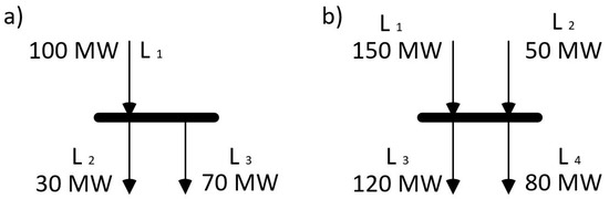
Figure 1.
Proportionality share principle: (a) bus with one source and two sinks and (b) bus with two sources and two sinks. Source may refer to line or generator, similarly as sink may refer to load or line.
Equation (1) defines the share of energy in line supplied that flows in each of line that feeds considered node. It is defined as a fraction of power flowing in this line over sum of power in all feeders [23].
Equation (2) allows the calculation of amount of flow in line that flows from line . It is calculated as product of and divided by sum of flows in all feeders . Which is further used for calculation for Figure 1b.
The basic principle is shown in the Figure 1a, where there is one source and two sinks. The total flow to the bus in the two lines is 100 MW, in which 70% (70 MW) is flowing in one line and 30% (30 MW) is flowing in the other one. The other example is in Figure 1b, which has two sources and two sinks. The calculation for this example gives results as below. The Equations (3) and (4) represent a generalization, in case there is more than one source as in Equation (2). For simplification purposes only active power was considered.
In this manner, we can present what is the share of the flow in the line, which supplies the power to load in particular nodes. Similarly, the share in the lines, which are supplied in power by generator in particular nodes. This relates to the way in which the generators use the power grid. Since the information given by this methodology can be introduced also from the opposite way—what is the share of power flow in line supplied to a load in considered node. This relates to the way in which the loads use the power grid. The methodology of PFT can also be addressed with the nodes, where there is more than one line supplying and more than one supplied line. The information may be used to know share of energy in a particular line flowing to the node, which is not directly connected.
Previous applications of Power Flow Tracing methods were mostly used to perform transmission cost allocation according to the actual usage of transmission lines by particular end consumers or eventually generators [17,18,20,21,28,31,32,35]. The high share of PFT usage was in apportionment of the losses, which could be assigned to the particular generators or loads according to their actual impact on losses [17,18,20,21,26,27,29,34,36].
In the literature, application of PFT in congestion management appears, although neither is it frequently used, nor does it use similar PFT methods. This idea was presented in [28,30,33], but it differs from research presented in this paper in methodology used to calculate PFT. In [28] the idea was to use Power Flow Comparison method, while in [30] the vectorgraph method was used, whereas in [33] the concept of using electrical distance was applied. In the [28], the method of power flow tracing is said to provide some signals to reduce the congestion by suggesting the increase or decrease in generation in specific generators and cause the opposite to another generator to keep the balance. The [29] paper takes into consideration not only active power but links it with the reactive power and considers its usage in congestion management on the basis of vectorgraphs. Whereas the [33] focuses as method in [28] only in suggesting the change in generation, and discusses the congestion in emergency states, due to n-1 contingency.
In this paper the concept of acting in case of congestion will be based on suggesting the nodes for increasing or decreasing the demand or generation, which was not previously presented in literature. Additionally, it is based on the cooperation with the active aggregators of RES and DER suited not only in the transmission system but also in the distribution system. Additionally, it is based on another, modified method of Inage domains.
3. Identification of the PFT Methods
3.1. Inage Domain Method
“Inage Domain” as algorithm was firstly presented by W. Mielczarski and E.M. Khan and as stated in [22,23] was used to calculate the network usage to assign network costs in Victorian power system in Australia and in the province of Ontario, Canada. It is based on the rules of proportionality of the flows. Additionally “Inage domain” algorithm shares the same idea of domains and commons as in [21]. Although it is based on the domains in a slightly different way, it applies the concept of domain to the lines, thus each branch may receive different coefficients. On the grounds of that, Inage Domain method and method presented in this research are more precise and detailed, due to calculation of coefficients for each element of the network. The original Inage Domain algorithm is presented in the following Figure 2.
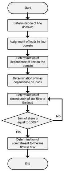
Figure 2.
Inage Domain algorithm. Sketch based on [22,23].
The algorithm may operate in two ways: it can present what is the share of the generators in the flow in the line—it is an upstream approach—or it can also calculate the share in the lines which supplies in power particular node—it is an downstream approach. In the following part of the article we will focus on the downstream approach. The algorithm has to follow further steps:
- Inage Domain of linesFirst of all, the Inage Domain of lines must be defined. The definition of Inage Domains of line l is the following—it is a set of branches that supplies line l in power. It is represented by Boolean approach, when the line belongs to the domain of l it takes value of 1, in other cases it takes 0.
- Assigning loads to line domainSecondly, the similar definition as in is used to assign the load to the domain. This stage defines if the particular load belongs to the domain of a given line.
- Identifying dependence of line on the domainThirdly, it is needed to define the contribution of the flow in line l from the other lines, which supplies the power to node n. It is possible to find the impact of power flowing in one line to the power flowing in the other line in the network. The dependence of line on the domain is based on the following equations.where is the load coefficient, is the power flowing in line between bus i and bus m, N is set of all the buses, which are connected to bus i and the flow is towards bus m, is the load in bus i, is the flow outflowing from the node i and between the nodes i and j, is the generation in the node i, is the generation coefficient, is the power flowing in line between bus q and bus i, N is all the buses, which are connected to bus i and the flow is towards bus i, C is contribution of line to line .
- Determining the load dependence on the lineIn the following point, it is needed to identify Inage Domain of load. Taking into consideration Inage Domain of demand—if the demand exists in a particular node and there is an inflow to the node, then it is considered as the demand/load is fully or in part supplied by the given line. The full contribution is when there is no outflow from that node. It is the share of the demand to the whole inflow to the node.where is the coefficient of load dependence on line, is the load in bus i, is the power flowing in line between bus q and bus i, N is all the buses, which are connected to bus i and the flow is towards bus i, is the generation in the node i.
- Identification of the commitment of load to the line flowThe following step is to determine the full commitment of the line to the load, where there is no direct connection between the load and the line. The contributions of the load, which is not connected directly with specific line, is given taking into consideration the impact of line on the line on the basis of already calculated contributions of lines. It is a sequential procedure, where the iterations are necessary.
The method requires consecutive steps to reach the commitment of all lines to all nodes equal to 100%. Similar procedure may be performed for upstream algorithm to calculate the use of lines by generators.
3.2. Modified Inage Domain Method
The method is based on common and domains idea, Inage Domain algorithm with modifications, which will be further explained. Main rule of original “Inage domain” algorithm is based on the finite number of iterations, which are replaced in the MID method by the generic equations. It implies no iterations, due to the program having general equations true to each node and calculates it all at once. Having the power flow, demands, generation as well as topology of the network, it is necessary to determine the directions of the flows. The MID algorithm is presented in the following Figure 3. The other modification made by the authors of the paper in comparison to the original Inage Domain method is shown in Equation (11), where the rule of proportionality of the flows is used directly.
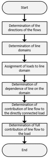
Figure 3.
Modified Inage Domain algorithm. Sketch developed by authors.
- At first the flows flowing into the node and the flows flowing out from the node for each line are named as flow received to the node and flow sent from the node. It creates two matrices, one per direction of flow. Both matrices have dimensions of , where n is number of nodes and l is number of lines. If line supplies the node with energy, then the element has a positive value of one and corresponding element in the second matrix has a value of zero. Second matrix is created in similar manner, the element has positive value, if the line is powered up by node. For both matrices, if line and node are not directly connected, then elements in both matrices are equal to zero.
- The second step covers determination of Inage Domain of lines. The line k belongs to Inage Domain of another line l, if the flow sending from the node n and flow receiving to the node are both positive.
- Thirdly, it is needed to define Inage Domains for loads. If, in node n the demand is located and the node n is supplied with energy by line k, then considered node and load belongs to Inage Domain of this line.
- Following step is to specify the approach to calculate dependence of line on the line . Value of for each pair of branches, that transports energy through the same node, is calculated as result of division of by . It is calculated directly on the basis of proportionality principle.
- The next step is the calculation of the value , which is the contribution of the line to the load. It defines factor of energy supplied to the node n, that is consumed in considered node. In other words, what portion of energy delivered by each line l is consumed by load in node n. Value is calculated by division of demand by inflow to node .
- The other shares are calculated taking into consideration Inage Domain of loads , existing demand in node and the value of the inflow to the node . It refers to the nodes, where no energy is transmitted—only to those where loads sink solely. Contribution of line to load in this case is calculated similarly as in previous point; however, it is multiplied by the Inage Domain of loads .Finally, the algorithm uses two last equations to calculate the contributions of line flows to the loads. Equation (14) is used to calculate contribution, if the node is only consuming the energy instead of transmitting it deeper into the network. It is shown by , which means that line k does not belong to the Inage Domain of any of line l. Due to the fact mentioned in previous sentence the contribution of line flows to nodes for this line is equal to calculated before value . Equation (15) covers the rest of cases—those when the energy is transmitted through the node, beside being consumed or not consumed at all. In that case at least one of line k connected to the node will belong to Inage Domain of another line l, what is represented by . In this instance the contribution of line flows to nodes for this line is the summation of product of dependence line on line and contribution of this line and contributions of load located in this node .
The aspect worth mentioning is that all of the shares are summing up to the 1 or 100%, which was also possible in “Inage Domain” method after some number of iterations, which was connected with the size of the network.
3.3. Consideration of Losses in MID Method
Frequently, PFT methods require loseless power flow. The method presented in this paper is flexible in this aspect—it is able to cope with lossy and loseless power flow. In the MID method the losses can be treated in two ways. The first way divides the losses of the line to halves and assigns those halves to the two nodes connected by this line. This approach is used in Equation (16), where is final load calculated with losses and is solely demand located in a particular node. It is a known method used to assign the losses to the nodes [17,18]. The definition, if connection between line and node exists, is determined by usage of connection matrix . Alternatively, the new concept presented in this paper is shown in Equation (17). It assigns the losses according to the PFT factors . It means the assignment of losses to the nodes, which causes the flow in line, where the losses occur. The node that is supplied in power by this line is responsible for losses in this line proportionally to its contribution in line flow.
3.4. Power Transfer Distribution Factor Method Adaptation
In the paper PTDF method is used in a modified way. Basic definition of PTDF covers the impact on transaction between node that sells energy and another that buys energy. Since the application of proposed methodology is rather restricted to balancing market or for use of transmission system operator, the PTDF are treated as singular change in demand in considered node. The model proposed in this research considers the transaction within the network as the increase of demand and the merit order defines needed change in the generation associated with the change of demand and additional losses. In other words, analysis measures impact of the change in demand on power flowing in lines in the network, whereas generation is adapting to this change according to merit order. The PTDF matrix has dimension to represent the influence of all n transactions in nodes on l lines. Additional demand was covered by the unit, that was able to cover it with the lowest cost with the consideration of lossy power flow.
4. Verification of the MID Method
In order to validate that presented method delivers comparable results, the comparison between Bialek’s PFT, Inage Domain and MID method is shown below. The verification is intended to confirm the correctness of the MID method with the methods which are established PFT methods.
4.1. Model of the Test Network
For the sake of simplicity, all of the discussions of results below are based on real power. Considerations are established on the network presented in Figure 4. The network consists of six buses, with five loads and two generators. They are connected by nine lines, where the direction of real power flow in each line is shown by the arrow next to the line. Values of loads and generation are shown in the figure, respectively in red and blue. Network data is presented in Table 1.
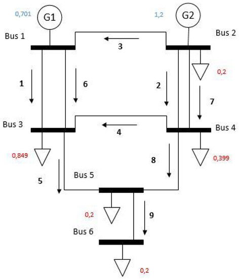
Figure 4.
Victorian Power Exchange network model with losses. The authors sketch based on [22].

Table 1.
Network data for Victorian Power Exchange system.
Table 1 provides full information about the analyzed network. Generation is located in first and second node, whereas in all nodes excluding first, load exists. Each line is described by starting node and ending node , correspondingly line flows are presented for both ends. Lines are named in such a manner to always obtain start and end bus compatible with direction of flow. However, the point of this action is to have a visibility on the network data, rather than simplification for algorithm, since it has no influence on it.
4.2. Comparison between MID Method and Białek’s Method
Due to the fact that Białek’s method is one of the well known and recognized methods, firstly the MID method will be compared with Białek’s method. Since Białek’s method [17,18] is adopted for lossless flows, the equivalent flows for the same power system but with lossless power flow is shown on the Figure 5. Step to transfer lossy power flow into lossless one is presented in [17]. It covers steps such as: calculation of average flows for each line and adaptation of nodal loads and generation to new flows to satisfy first Kirchhoff law. Results of this action are presented in the Figure 5, whereas original power flow is shown in Table 1.
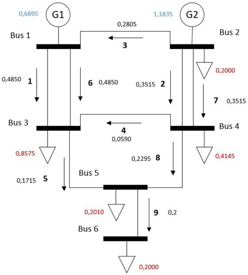
Figure 5.
Victorian Power Exchange network model without losses. Sketch developed by authors.
Białek’s and MID methods will be presented for lossless flow. The results of PFT factors in downstream approach for the new method are presented in Table 2. Downstream power flow tracing factors are calculated for all the lines and nodes except the first one, where the demand does not exist. The number in the box (in Table 2) means that the share of power delivered by third line to sixth node is 0.0831. In other words, the flow in line is responsible for powering particular load in . The differences of results between Białek’s method and the MID method are below and can be neglected.
Table 2.
PFT factors from MID method—downstream approach.
Moving forward to the upstream approach, those factors are shown in Table 3. The power flow tracing factors are calculated for all the lines and for nodes where the generation is located. The PFT factor in this approach defines what share of power flow in specific line was caused by considered generator. For instance (see box in Table 3) the share of the first generator in the flow in line six is equal to 0.7108, or 71.08%. The difference of results between Białek’s method and the MID method, as previously mentioned, are negligible. The difference between the shares of PFT factors is below , which is probably lower than required for any application known by authors.
Table 3.
PFT factors from MID method—upstream approach.
4.3. Comparison between MID Method and Inage Domain Method
The following step will contain the comparison between MID method presented in this article and an original Inage Domain method, due to the fact that they are mostly based on the same principles, however adopted differently. The target was to compare the method presented in this article with the original Inage Domain method. The MID method shows values which are summing up to unity in Table 2, whereas the results from [22], given in Table 4 and Table 5, do not sum up to unity in some cases. This may be an outcome of having results from iteration, which could not be the final one. The highest difference may be found in the 2nd and 7th line. Despite that, both lines should have the same PFT, as they are parallel lines and those lines are supplied by the same node, which is “perfect mixer”. When the methods are compared, the difference occurs between line 2nd and 7th—both connect the same nodes. Error for downstream algorithm is defined as a result of subtraction of factor of MID method from factor of Inage Domain method and further divided by factor of MID method, expressed as percentage. Error between methods is presented in the Figure 6.
Table 4.
PFT factors from original Inage Domain method-downstream approach.
Table 5.
PFT factors from original Inage Domain method-upstream approach.
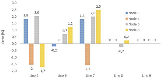
Figure 6.
Percentage error between original Inage Domain and MID method in downstream approach. Presented errors for nodes that participate in any flow for lines 6–9.
In Figure 6, the difference between PFT factors from both methods is presented. The error is determined with an assumption that MID method shows reference values, what was proven in the previous subsection by comparison to Białek’s method.
The chart presents error of original Inage Domain method compared to MID method. The graph is constructed in a way in which each column in different color describes the error in share of different node in power flow in considered line described on horizontal axis. Those nodes are arranged in groups of four to present the errors in shares for each line. Moreover, an interesting case can be found, when comparing the error as it was presented previously in 2nd and 7th line. Probably, the errors in share in 2nd and 7th line are caused by the fact that those lines are located further from the load than other lines. Errors should be equal since lines are parallel and should have the same PFT factors. However, the original Inage Domain method has different factors for them. Such a case may be caused by the fact that results are not presented for the final iteration.
Moving forward, the results of the upstream approach of the original Inage domain method are shown in the Table 5 and the errors between original method and MID method are shown in the Figure 7. Similarly as previously, error in upstream algorithm is defined as a result of subtraction of factor of MID method from factor of Inage Domain method and further divided by factor of MID method, expressed as percentage. The errors regarding the first and second generator differs in the sign, due to the fact that in both methods sum of shares is equal to unity, thus if the share of one generator was higher, then for the second it has to be lower. For most of the lines, the original Inage Domain method has lower share for the second generator. The highest difference regarding first generator can be found for the 1st and 6th line, as they are parallel. Next highest error can be observed in the 5th line. Probably the error is a result of different consideration of losses. The original method is calculated for lossy power flow, whereas the modified method is based on lossless power flow obtained from the same lossy flow.
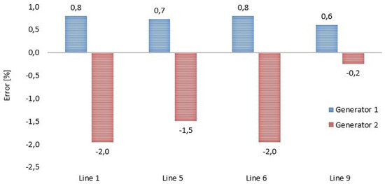
Figure 7.
Percentage error between original Inage Domain and MID method in upstream approach.
On the basis of comparison with Bialek PFT, the new MID method may be considered as verified, because it delivers the identical results. Thus it may be applied for the purpose of transmission cost allocation or in applications in advanced congestion management. Additionally, the method has advantages over original Inage Domain method, which was shown on the basis of comparison of both methods.
5. Application of the Mid Method
This section provides a comprehensive review of possible applications of MID method. The application, which will be reviewed using MID method will be the following:
- Allocation of transmission cost.
- Application in modern power system for advanced congestion management.
The most frequently used application of PFT method will be shown, which is the allocation of transmission cost as presented in [22,23]. Additionally, the application of PFT method will cover aspects of active system management in modern power system, in which the congestion management will be performed with adaptation of the demand or generation in the node to reduce or remove congestion. The point of the presented applications is to highlight possible utilization to solve currently existing issues. The MID method will be applied into the larger system, which will consist of 14 buses, 10 with generation and all with loads. In total, the network is built of 19 lines. The 14 bus test system is presented in Figure 8. Details of power flow for both applications can be found in Appendix A.
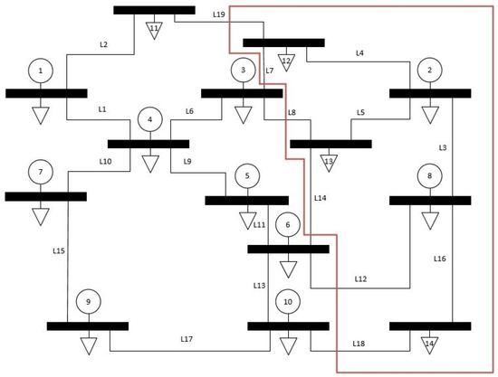
Figure 8.
The 14-bus test system. Sketch developed by authors.
5.1. Application of MID Method in the Allocation of Transmission Cost
Transmission cost allocation is a well known problem in liberalized power systems. This subsection is focused on possible application of MID method in this area. Aspects such as social approval of differentiation of network cost or ratio between fixed and variable operation and maintenance costs are out of scope of this paper. It is needed to mention that the parameters describing the state of the network vary between Section 5.1 and Section 5.2, which is shown in the Appendix A. An illustrative example of MID method usage presents possibility to adopt method in transmission cost allocation. The results, presented in Figure 9, were reduced to the part of the system marked in red color in the Figure 8 to improve visibility. There are lines, as 16th and 18th, which power solely in this particular case node 14. Although the same share can be found in the lines which supply the power to the same node, as 3th and 12th. It is directly implied by “perfect mixer” assumption. In other words, it is the foundation of the basic principle of the “perfect mixer”, which assigns the same share of usage to the lines, whose flow is supplying the bus, in case of downstream approach.
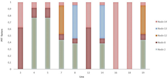
Figure 9.
PFT shares of line usage by nodes according to MID method.
Therefore, the comparison of MID method with postage stamp method is performed due to the fact that postage stamp method is frequently used to allocate costs of network. For this comparison the equal total costs for each line are assumed, whereas the price of energy is out of scope. To simplify calculation, the total cost of each line that has to be allocated is equal to unity.
The Equation (18) calculates cost of network usage on the basis of postage stamp method. Total network cost is assigned proportionally to the ratio between power installed in node and sum of total power installed .
The Equation (19) defines a possible way to use MID method to assign network costs to nodes . It is calculated by multiplication of line cost and calculated PFT factor accordingly to MID method . Finally, those products are summed for each node to calculate total cost for each node. The method uses actual flow, rather than installed power, which is more accurate. However, it requires multiple calculation in time to cover different power flows patterns.
The Figure 10 shows the results of distribution of the network costs among nodes by two methods: postage stamp method used frequently (according to Equation (18)) and application of MID method for this purpose (according to Equation (19)). Illustration of differences should cover at least nodes 2, 5 and 14. In case of the first one—node five, new method assigns no cost, since it is directly supplied by generation located in this node, due to the fact that any line supplies this node. However, when node 2nd and 14th are investigated, then it is noticeable that both are relatively far from actual generation and both are participating largely in flows from supplying lines. The fact that both have one of the highest demands is also meaningful for calculation of both costs. However, it influences stronger method based on PFT, since it is based on temporal power flow, which may not reflect typical network usage, whereas the postage stamp method is based on the installed power, which may not reflect actual usage at all.
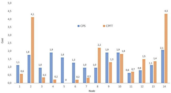
Figure 10.
Network costs for nodes in postage stamp method (CPS) and MID power flow tracing method (CPFT).
The values may differ according to the assumed ratio between costs divided equally and differentiated among nodes. To sum up, this method may be used in transmission cost allocation. Moreover, if it is compared to postage stamp, it reflects real network usage. However, cost allocation should not be based on single power flow pattern to properly reflect network usage in different conditions.
5.2. Application of MID Method in Modern Power Systems for Advanced Congestion Management
The active system management will be crucial in the modern power systems with high share of renewable energy. It will gain significant attention, due to the increasing number of congestion in the network. The solution may be to use PFT method in order to seek and find the nodes with active agents, where the acceptance of offer from agent will help dismantle the congestion in the most effective way. The PFT may be used in market approach to congestion management and in arbitrary decisions. In the first case, it may be a tool for market or system operator to inform participants about network state and provide useful information about congestion. In the case of non market approach, it may contribute by providing additional overview of how congestion may be dismantled and where the same action may result in more efficient use of resources.
This section is intended to show:
- The selection of the nodes suggested by MID method will be corresponding with the choice performed by using PTDF method.
- Change in cost, due to possible decrease of the demand in specific place in the network.
The following example is based on network shown in Figure 8. In tables below, the PFT factors are presented, from upstream approach in Table 6 and from downstream approach in Table 7. The tables do not contain the nodes, which do not participate in the flow of considered lines. In the considered case, the first and sixth line are congested, which means that limitation of maximal line flow induces non optimal commitment and dispatch, due to the fact that the PFT factors are only presented regarding those lines. The chosen nodes to decrease the power outflowing from the node are: node 4, node 5 and node 7. In those nodes, increase of demand or decrease of power generation may reduce congestion. Respectively the nodes to increase power outflowing from the node are in case of the first line: node 1, node 11 and 12, whereas in case of sixth line the nodes are: 2, 3, 12 and 13. Inversely to the previous, the decrease of demand or increase of generation may resolve the congestion. The threshold of 0.1 is set as minimal considered value of PFT, as potentially able to influence the congestion.
Table 6.
PFT factors from Modified Inage Domain method—upstream approach.
Table 7.
PFT factors from Modified Inage Domain method—downstream approach.
To validate that chosen nodes will be able to effectively change the flow in the congested line, the choice of nodes by PFT method is compared to the choice resulting from PTDFs as reference, presented in Table 8. The PTDFs are commonly used to show the dependency between change in demand or generation and the flow in line. The main target is to find if the PFT and PTDF will show the same nodes and if those chosen nodes may reduce or dismantle congestion.
Table 8.
Power Transfer Distribution Factors.
The highest increase in first line flow is noted when the demand in one of nodes: 1st, 11th and 12th is increased, which is reflected by PTDFs. The meaning of this is if there is a need to reduce the flow in the congested line, then it is needed to decrease the demand in those nodes, or alternatively increase the generation in those nodes. The chosen nodes which have the highest share (1, 11 and 12) are the same nodes as chosen using PFT method.
The main point of PTDF method is to indicate in which node the increase in demand will decrease flow in line. When first line is considered the nodes 4th, 5th, 7th and 9th may reduce flow in line by increasing demand. The chosen nodes according to PTDF method are matching (except 9th) with the chosen nodes according to the MID method. In the following part of this section the influence of change in demand in nodes will be investigated further.
Since both methods choose the same sets of nodes as with the potentially highest influence, correspondence between them is proven. However, the next paragraph describes adaptation of this choice to power system. To verify if the choice is correct, the values of the prices that may be paid for each megawatt hour of reduced demand in node of 20 MWh reduction in considered hour are presented on Figure 11.
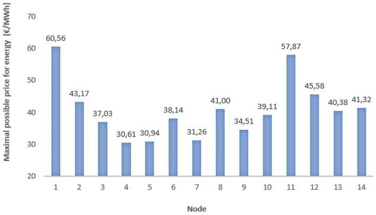
Figure 11.
The values of the prices that may be paid for each megawatt hour in case of reduced demand in the node of 20 MWh reduction.
In other words, the price shown on the chart (Figure 11) represents maximal value of price that may be paid for demand response in case of congestion. Value is based on two complete power flow, commitment and dispatch solutions. It is obtained by subtracting total cost of scenario (when in one of the nodes demand is reduced by value of 20 units [MW] during one hour) from reference case, where congestion is dismantled by solely redispatch of conventional power plants in the same conditions.
This change in cost could be offered to the active agent in distribution system, who may decrease its demand to reduce flows in overloaded line. It may give benefits, as decrease of cost of the whole system, if the price given to the active agent would be lower than the presented one. Additionally, it may decrease a flow in the congested line. In a reference to values of PFT from MID method, the two highest values are in nodes chosen by PFT and thus the choice of nodes allows to present, in which node operator may offer highest price for the same service.
On the basis of results presented in this section, the method is considered as applicable in transmission cost allocation and in advanced congestion management. Moreover, the application in area of congestion management was presented in two options, where the method is applied as a tool for system operator and as the additional information for market participants.
6. Conclusions
Evolution of power systems, especially the development of RES, is influencing the patterns of power flow in the network. Previously power flow was controlled mainly by large, centrally dispatched, thermal power plants, whereas now it is strongly tied with weather conditions, due to increase of generation from RES. Moreover, previous investments in network were planned to be able to cope with investment in generation, both having similar investment cycles in terms of duration. Nowadays, dynamic growth of installed capacity of RES has shorter delays and overall project duration is shorter, which does not allow network investment to prepare for adequate plans and projects.
The paper presented a new approach of dismantling the congestions in the transmission network with the usage of active aggregators or active agents from distribution network. The flexibility services, which will be provided, contain the selection of the nodes between transmission and distribution system, which will dismantle the congestion by decreasing or increasing the demand or generation. The tool which will be indispensable in this process will be PFT method, or more precisely new MID method. The paper presented main principles of the Modified Inage Domain method on the grounds of Inage Domain method. The correctness of the MID method was proved by comparison with Inage Domain method and PFT method developed by Białek. The MID method gives the same or similar results; if there is a difference, it is negligible.
The possible applications of MID methods as the allocation of transmission cost and application in modern power systems for advanced congestion management were shown in the paper. The MID method may be applied in the allocation of transmission cost in comparison to the postage stamp method—it reflects better, real network usage. Although it should not be based on single power flow pattern, it is possible to create flow patterns depending on the season, situation or weather conditions. It has been proven that MID method can be applied to advanced congestion management problem by comparing the sets of chosen nodes with the PTDFs results. The MID method chose the same sets of nodes by giving the highest influence on dismantling the congestion. What is more, the maximal value of price that may be paid for demand response in case of congestion, is the highest in chosen nodes, which also has the highest influence on dismantling the congestion. This allows one to present which node operator may offer the highest price for the same service.
This paper presented the fact that MID method gives comparable results to well recognized methods and may replace other methods in their applications, due to its simplicity and straight forward steps. Moreover, the authors believe that new models of energy market will require appliances such as MID method. The paper showed possible application of new method and benefits from the use of it.
Author Contributions
A.B. and W.N. contributed equally to this work and all of its stages and elements. All authors have read and agreed to the published version of the manuscript.
Funding
This research received no external funding.
Acknowledgments
The author of this article would like to express deep sense of thanks to the FICO® Corporation for providing academic licenses for Xpress Optimization Suite to Institute of Electrical Power Engineering at Lodz University of Technology. The authors of this article would like to express sincere gratitude to the reviewers for providing insightful comments and valuable improvements to our manuscript.
Conflicts of Interest
The authors declare no conflict of interest.
Abbreviations
The following abbreviations are used in this manuscript:
| AC | Alternating Current |
| DC | Direct Current |
| DER | Distributed Energy Resources |
| DSO | Distribution System Operator |
| EU | European Union |
| GGDF | Generalized Generator Distribution Factor |
| IEEE | Institute of Electrical and Electronics Engineers |
| LV | Low Voltage |
| MID | Modified Inage Domain |
| MV | Medium Voltage |
| PFT | Power Flow Tracing |
| PST | Phase Shifting Transformers |
| PTDF | Power Transfer Distribution Factors |
| PV | Photovoltaic |
| RED | Relative Electrical Distance |
| RES | Renewable Energy Sources |
| TSO | Transmission System Operator |
Appendix A
Appendix A.1. Application of Mid Method in Transmission Cost Allocation
Table A1.
Parameters of state of the network for 5.1.
Table A1.
Parameters of state of the network for 5.1.
| L\N | Flow | ’From’ n | ’To’ n | Susc. | Cond. | Dem. | Gen. | Loss | P. instal. |
|---|---|---|---|---|---|---|---|---|---|
| 1 | −345.04 | 1 | 4 | 72 | 0.90 | 147.75 | 0 | 7.26 | 350 |
| 2 | 190.04 | 1 | 11 | 152 | 1.90 | 207.93 | 0 | 3.70 | 550 |
| 3 | 62.33 | 2 | 8 | 126 | 1.58 | 105.13 | 0 | 11.28 | 300 |
| 4 | −140.38 | 2 | 12 | 82 | 1.03 | 229.30 | 798.0 | 16.81 | 600 |
| 5 | −133.58 | 2 | 13 | 84 | 1.05 | 211.07 | 727.4 | 7.62 | 500 |
| 6 | −441.32 | 3 | 4 | 82 | 1.03 | 149.57 | 536.0 | 11.55 | 400 |
| 7 | 139.97 | 3 | 12 | 44 | 0.55 | 135.32 | 400.0 | 5.78 | 300 |
| 8 | 184.95 | 3 | 13 | 56 | 0.70 | 175.35 | 0 | 5.08 | 300 |
| 9 | −298.02 | 4 | 5 | 88 | 1.10 | 235.91 | 0 | 6.17 | 600 |
| 10 | 63.54 | 4 | 7 | 82 | 1.03 | 225.16 | 0 | 6.43 | 600 |
| 11 | 210.73 | 5 | 6 | 20 | 0.25 | 75.61 | - | 3.53 | 200 |
| 12 | 224.43 | 6 | 8 | 62 | 0.78 | 105.53 | - | 4.95 | 250 |
| 13 | 275.23 | 6 | 10 | 72 | 0.90 | 132.32 | - | 5.00 | 350 |
| 14 | 85.95 | 6 | 13 | 56 | 0.70 | 227.79 | - | 2.54 | 650 |
| 15 | 322.44 | 7 | 9 | 44 | 0.55 | ||||
| 16 | 106.33 | 8 | 14 | 62 | 0.78 | ||||
| 17 | 80.35 | 9 | 10 | 28 | 0.35 | ||||
| 18 | 123.99 | 10 | 14 | 82 | 1.03 | ||||
| 19 | 110.90 | 11 | 12 | 44 | 0.55 |
“From” n: Considered as starting node for line l; “To” n: Considered as ending node for line l; Susc.: Suceptance; Cond.: Conductance; Dem.: Demand; Gen.: Generation; P. instal.: Power installed.
Appendix A.2. Application of Mid Method in Modern Power Systems for Advanced Congestion Management
Table A2.
Parameters of state of the network for 5.2.
Table A2.
Parameters of state of the network for 5.2.
| L\N | Flow | ’From’ n | ’To’ n | Susc. | Cond. | Dem. | Gen. | Loss | P. instal. |
|---|---|---|---|---|---|---|---|---|---|
| 1 | −443.27 | 1 | 4 | 72 | 0.90 | 212.32 | 0 | 9.29 | 350 |
| 2 | 221.66 | 1 | 11 | 152 | 1.90 | 387.55 | 0 | 4.29 | 550 |
| 3 | −117.28 | 2 | 8 | 126 | 1.58 | 163.61 | 300.00 | 12.84 | 300 |
| 4 | −135.82 | 2 | 12 | 82 | 1.03 | 384.19 | 798.00 | 17.68 | 600 |
| 5 | −138.74 | 2 | 13 | 84 | 1.05 | 303.32 | 800.00 | 7.29 | 500 |
| 6 | −366.83 | 3 | 4 | 82 | 1.03 | 307.58 | 598.00 | 9.83 | 400 |
| 7 | 215.65 | 3 | 12 | 44 | 0.55 | 179.23 | 650.00 | 6.68 | 300 |
| 8 | 274.72 | 3 | 13 | 56 | 0.70 | 322.06 | 421.51 | 5.61 | 300 |
| 9 | −280.18 | 4 | 5 | 88 | 1.10 | 369.49 | 162.00 | 6.92 | 600 |
| 10 | −133.79 | 4 | 7 | 82 | 1.03 | 360.30 | 262.00 | 7.05 | 600 |
| 11 | 209.22 | 5 | 6 | 20 | 0.25 | 140.93 | - | 3.30 | 200 |
| 12 | 175.03 | 6 | 8 | 62 | 0.78 | 151.66 | - | 5.61 | 250 |
| 13 | 197.05 | 6 | 10 | 72 | 0.90 | 246.62 | - | 7.10 | 350 |
| 14 | 117.73 | 6 | 13 | 56 | 0.70 | 354.50 | - | 4.67 | 650 |
| 15 | 330.29 | 7 | 9 | 44 | 0.55 | ||||
| 16 | 151.59 | 8 | 14 | 62 | 0.78 | ||||
| 17 | 115.88 | 9 | 10 | 28 | 0.35 | ||||
| 18 | 207.58 | 10 | 14 | 82 | 1.03 | ||||
| 19 | 77.43 | 11 | 12 | 44 | 0.55 |
References
- EU. European Union Directive (EU) 2018/2001 on the promotion of the use of energy from renewable sources. Off. J. Eur. Union 2018, 2018, 1–128. [Google Scholar]
- Leiva, J.; Carmona Pardo, R.; Aguado, J.A. Data Analytics-Based Multi-Objective Particle Swarm Optimization for Determination of Congestion Thresholds in LV Networks. Energies 2019, 12, 1295. [Google Scholar] [CrossRef]
- Esmat, A.; Usaola, J.; Moreno, M.Á. Distribution-Level Flexibility Market for Congestion Management. Energies 2018, 11, 1056. [Google Scholar] [CrossRef]
- Union of the Electricity Industry-EURELECTRIC. Flexibility and Aggregation Requirements for Their Interaction in the Market. January 2014. Available online: https://cdn.eurelectric.org/media/1845/tf_bal-agr_report_final_je_as-2014-030-0026-01-e-h-5B011D5A.pdf (accessed on 31 May 2020).
- CEDEC; EDSOE; ENTSO-E; EURELECTRIC; GEODE TSO-DSO. Report—An Integrated Approach to Active System Management; CEDEC; ENTSO-E; GEODE; E.DSO; EURELECTRIC: Berlin, Germany, 2019. [Google Scholar]
- Swain, K.P.; De, M. Congestion Management Using Demand Response in Smart Distribution System. In Proceedings of the 2019 IEEE Region 10 Symposium, Kolkata, India, 7–9 June 2019; pp. 485–490. [Google Scholar]
- Li, J.; Li, F. A congestion index considering the characteristics of generators & networks. In Proceedings of the 47th International Universities Power Engineering Conference, London, UK, 4–7 September 2012; pp. 1–6. [Google Scholar]
- Singh, A.K.; Özveren, C.S. Congestion pricing in a deregulated market using A.C. Power Transfer Distribution Factors. In Proceedings of the 50th International Universities Power Engineering Conference, Stoke on Tren, UK, 1–4 September 2015; pp. 1–6. [Google Scholar]
- Nabavi, S.M.H.; Jadid, S.; Masoum, M.A.S.; Kazemi, A. Congestion management in nodal pricing with genetic algorithm. In Proceedings of the International Conference on Power Electronic, Drives and Energy Systems, New Delhi, India, 12–15 December 2006; pp. 1–5. [Google Scholar]
- Nappu, M.B.; Saha, T.K. A comprehensive tool for congestion-based nodal price modelling. In Proceedings of the IEEE Power & Energy Society General Meeting, Calgary, AB, Canada, 26–30 July 2009; pp. 1–8. [Google Scholar]
- Kumar, J.; Kumar, A. Multi-transactions ATC determination using PTDF based approach in deregulated markets. In Proceedings of the Annual IEEE India Conference, Hyderabad, India, 16–18 December 2011; pp. 1–6. [Google Scholar]
- Zhou, Q.; Bialek, J.W. Approximate model of European interconnected system as a benchmark system to study effects of cross-border trades. IEEE Trans. Power Syst. 2005, 20, 782–788. [Google Scholar] [CrossRef]
- Bhaskar, M.A.; Jimoh, A.A. Available transfer capability calculation using PTDF and implementation of optimal power flow in power markets. In Proceedings of the IEEE International Conference on Renewable Energy Research and Applications, Birmingham, UK, 20–23 November 2016; pp. 219–223. [Google Scholar]
- Naik, R.S.; Vaisakh, K.; Anand, K. Determination of ATC with PTDF using linear methods in presence of TCSC. In Proceedings of the 2nd International Conference on Computer and Automation Engineering, Singapore, 26–28 February 2010; pp. 146–151. [Google Scholar]
- Leveringhaus, T.; Hofmann, L. Comparison of methods for state prediction: Power Flow Decomposition (PFD), AC Power Transfer Distribution factors (AC-PTDFs), and Power Transfer Distribution factors (PTDFs). In Proceedings of the IEEE PES Asia-Pacific Power and Energy Engineering Conference, Hong Kong, China, 7–10 December 2014; pp. 1–6. [Google Scholar]
- Cheng, X.; Overbye, T.J. PTDF-based power system equivalents. IEEE Trans. Power Syst. 2005, 20, 1868–1876. [Google Scholar] [CrossRef]
- Bialek, J. Tracing the flow of electricity. IEE Proc. Gener. Transm. Distrib. 1996, 143, 313–320. [Google Scholar] [CrossRef]
- Bialek, J. Identification of source-sink connections in transmission networks. In Proceedings of the Fourth International Conference on Power System Control and Management, London, UK, 16–18 April 1996. [Google Scholar]
- Singh, S. Power Tracing in a Deregulated Power System: IEEE 14-Bus Case. Int. J. Comput. Technol. Appl. 2012, 3, 887–894. [Google Scholar]
- Narimani, M.; Hosseinian, S.H.; Vahidi, B. A modified methodology in electricity tracing problems based on Bialek’s method. Int. J. Electr. Power Energy Syst. 2014, 60, 74–81. [Google Scholar] [CrossRef]
- Kirschen, D.; Allan, R.; Strbac, G. Contributions of individual generators to loads and flows. IEEE Trans. Power Syst. 1997, 12, 52–60. [Google Scholar] [CrossRef]
- Mielczarski, W. Handbook: Energy Systems & Markets, 1st ed.; Association of Polish Electrical Engineers, Division Łódź; Institute of Electric Power Engineering, Lodz University of Technology: Lodz, Poland, 2018; ISBN 978-83-940283-4-3. [Google Scholar]
- Mielczarski, W. Rynki Energii Elektrycznej, 1st ed.; ARESA: Warsaw, Poland, 2000; ISBN 83-87574-35-X. [Google Scholar]
- Baczyńska, A. A new approach to constraints removal using Power Flow Tracing method. In Proceedings of the 16th International Conference on the European Energy Market (EEM), Ljubljana, Slovenia, 18–20 September 2019; pp. 1–5. [Google Scholar]
- Wu, F.F.; Ni, Y.; Wei, P. Power transfer allocation for open access using graph theory-fundamentals and applications in systems without loopflow. IEEE Trans. Power Syst. 2000, 15, 923–929. [Google Scholar] [CrossRef]
- Macqueen, C.N.; Irving, M.R. An algorithm for the allocation of distribution system demand and energy losses. IEEE Trans. Power Syst. 1996, 11, 338–343. [Google Scholar] [CrossRef]
- Mustafa, M.W.; Shareef, H. A Comparison of Electric Power Tracing Methods Used in Deregulated Power Systems. In Proceedings of the IEEE International Power and Energy Conference, Putra Jaya, Malaysia, 28–29 November 2006; pp. 156–160. [Google Scholar]
- Yang, J.; Anderson, M.D. Tracing the flow of power in transmission networks for use-of-transmission-system charges and congestion management. In Proceedings of the IEEE Power Engineering Society 1999 Winter Meeting, New York, NY, USA, 31 January–4 February 1999; pp. 399–405. [Google Scholar]
- Abdelkader, S. Determining generators’ contribution to loads and line flows & losses considering loop flows. Int. J. Electr. Power Energy Syst. 2008, 30, 368–375. [Google Scholar] [CrossRef]
- Wang, H.; Bao, H. A new method of congestion management based on power flow tracing. In Proceedings of the China International Conference on Electricity Distribution, Xi’an, China, 10–13 August 2016; pp. 1–4. [Google Scholar]
- Zobian, A.; Ilic, M.D. Unbundling of transmission and ancillary services. I. Technical issues. IEEE Trans. Power Syst. 1997, 12, 539–548. [Google Scholar] [CrossRef]
- Barcia, P.; Pestana, R. Tracing the flows of electricity. Int. J. Electr. Power Energy Syst. 2010, 32, 329–332. [Google Scholar] [CrossRef]
- Masaki, E.; Ogawa, T.; Ohtaka, T.; Iwamoto, S.; Ochi, T. Lineflow congestion elimination using generator power flow tracing method. In Proceedings of the International Conference on Power System Technology, Singapore, 21–24 November 2004; pp. 850–855. [Google Scholar]
- Chang, Y.C.; Lu, C.N. An electricity tracing method with application to power loss allocation. Int. J. Electr. Power Energy Syst. 2001, 23, 13–17. [Google Scholar] [CrossRef]
- Visakha, K.; Thukaram, D.; Jenkins, L. Transmission charges of power contracts based on relative electrical distances in open access. Electr. Power Syst. Res. 2004, 70, 153–161. [Google Scholar] [CrossRef]
- Reta, R.; Vargas, A. Electricity tracing and loss allocation methods based on electric concepts. IEE Proc. Gener. Transm. Distrib. 2001, 148, 518–522. [Google Scholar] [CrossRef]


© 2020 by the authors. Licensee MDPI, Basel, Switzerland. This article is an open access article distributed under the terms and conditions of the Creative Commons Attribution (CC BY) license (http://creativecommons.org/licenses/by/4.0/).