Integration of Joint Power-Heat Flexibility of Oil Refinery Industries to Uncertain Energy Markets

Abstract

This paper proposes a novel approach to optimize the main energy consumptions of heavy oil refining industries (ORI) in response to electricity price uncertainties. The whole industrial sub-processes of the ORI are modeled mathematically to investigate the joint power-heat flexibility potentials of the industry. To model the refinery processes, an input/output flow-based model is proposed for five main refining units. Moreover, the role of storage tanks capacity in the power system flexibility is investigated. To hedge against the electricity price uncertainty, an uncertain bound for the wholesale electricity price is addressed. To optimize the industrial processes, a dual robust mixed-integer quadratic program (R-MIQP) is adopted; therefore, the ORI’s operational strategies are determined under the worst-case realization of the electricity price uncertainty. Finally, the suggested approach is implemented in the south-west sector of the Iran Energy Market that suffers from a lack of electricity in hot days of summer. The simulation results confirm that the proposed framework ensures industrial demand flexibility to the external grids when a power shortage occurs. The approach not only provides demand flexibility to the power system, but also minimizes the operation cost of the industries.

1. Introduction

1.1. Motivation and Problem Description

The Iran Energy Market (IEM) has been experiencing two major challenges recently. First of all, the Iran Power Grid (IPG) faces high peak demands during hot days of summer when the electricity demand of the air conditioning systems increases dramatically [1]. Increasing the generation and transmission capacities of the electricity network is a controversial decision. The reason is that the electricity network has a high unused non-seasonal capacity in summer. Therefore, it cannot be an economic decision to make such a huge investment. To overcome the challenge, there are some flexibility potentials among the heavy industries that can provide demand flexibility to the electricity/gas network [2]. Since Iran is now beginning to emerge as the major refiner in the Middle East in terms of refining capacity, the electricity and heat generation of Iran’s Oil Refinery Industries (ORI) can provide a golden opportunity to hedge against the energy shortage at peak hours.

1.2. Literature Review

Generally, the ORI or petroleum refinery is an industrial process plant where crude oil is transformed and refined into more useful products, such as petroleum naphtha, gasoline, diesel fuel, asphalt base, heating oil, kerosene, liquefied petroleum gas, jet fuel, and fuel oils [3]. The ORI consumes a large amount of energy, i.e., electricity and heat, and steam for the refinery processes. Conventionally, the ORI is equipped with self-generation facilities, e.g., cogeneration units, to supply the industrial processes with electricity and steam. Producing/consuming the electricity and heat in refinery processes simultaneously, the energy management of the ORI is a complex problem. Therefore, barely comprehensive research studies are conducted, especially in the field of electrical energy management.

In the literature on the ORI, most research studies were focused on two issues, as follows:

(1)

Optimization of oil and gas productions.

(2)

Energy efficiency measures in the ORI equipment.

First of all, in 2010, a research study was conducted in Gabriel Passos Refinery of Brazil to suggest additional investments, to expand its current production scheme [4]. Later, in 2011, a short-term scheduling problem of crude oil operations was provided to overcome the crude oil residency time constraint [5]. In 2012, a conceptual framework was addressed to predict the fouling rate in an industrial crude oil pre-heater using the computational fluid dynamic technique [6]. In 2013, four heat supply alternatives were studied to investigate the role of utilizing excess heat on the energy cost of the ORI [7]. In 2014, a comprehensive study was done in Mexico to reschedule the industrial equipment of the ORI. The main aims were to optimize the operation cost and improve power quality [8]. In 2015, a multi-period optimizing model was suggested to schedule a fuel gas system within refining processes. The main contribution of the study was to model the pipeline system which was usually ignored in the previous studies [9]. In 2016, paper [10] suggested three integrated oil shale refinery processes to turn losses of the conventional oil shale process into profits at the situation of low oil prices. In 2017, a research study investigated the possibility of operating the thermal desalination plants by waste gases. This paper studied the use of waste gas that emerged from oil refineries rather than burning in the air [11]. In 2018, a novel method for real-time data validation was developed in the ORI using sensor data from the power and petrochemical plants of refining processes [12]. Finally, an energy recovery solution is offered for the pump-as-turbine technology applied in the ORI in 2019 [13].

As the literature reveals, the main concentration of the previous studies is on the optimization of ORI productions and equipment. In this way, very limited studies were focused on the energy management of the ORI to integrate the refining demand flexibility to external networks.

Based on the abovementioned facts, to the best of our knowledge, only four research studies were conducted in the area of energy management of the ORI. First of all, paper [14] presented a generalized formulation to determine the optimal operating strategy of industrial cogeneration schemes in terms of electricity and heat. The main contribution of this study was that the suggested approach addressed the grid connection to provide the demand flexibility to any kind of industry. Later, a prominent study was done to determine the flexibility potentials of the ORI among different refining processes [15]. In this study, a flow diagram was presented for Kwinana Refinery of Australia to describe what refining processes have the ability to interrupt and/or delayed start. Although this study suggested the flexibility potentials of the refining processes, the applicability of the suggested flexibilities is still a challenge due to not simulating the approach. Finally, a prominent study was conducted recently to integrate the flexibility potentials of the ORI into the external power grid [16]. It is the first time that a study has simulated the operational processes of the ORI to provide demand flexibility to the power system in response to the demand response signals. Although this paper initiates the determination of ORI flexibilities, it fails to investigate the whole flexibility potentials among the refining processes. The reason is that the study models the crude distillation units only, and supposes that the other processing units are appropriately designed to continuously process the input flow of the materials. Therefore, the possible flexibilities of the non-modeled processing units remain unknown.

To sum up the literature, Figure 1 depicts a schematic diagram to show the main objectives of the previous studies in the ORI [17,18,19,20,21,22]. Furthermore, it determines the clear need for future studies.

As the flowchart reveals, the oil production optimization and the energy consumption efficiency are two main objectives of the studies in the first and last decades of the current century, respectively. Increasing the electrical demand in power systems, demand-side flexibility is a clear need for future power systems. Therefore, despite the two abovementioned objectives, the ORI processes should be optimized to provide flexibility potential to power systems. Consequently, the integration of ORI flexibility to power grids is an essential requirement for future power systems.

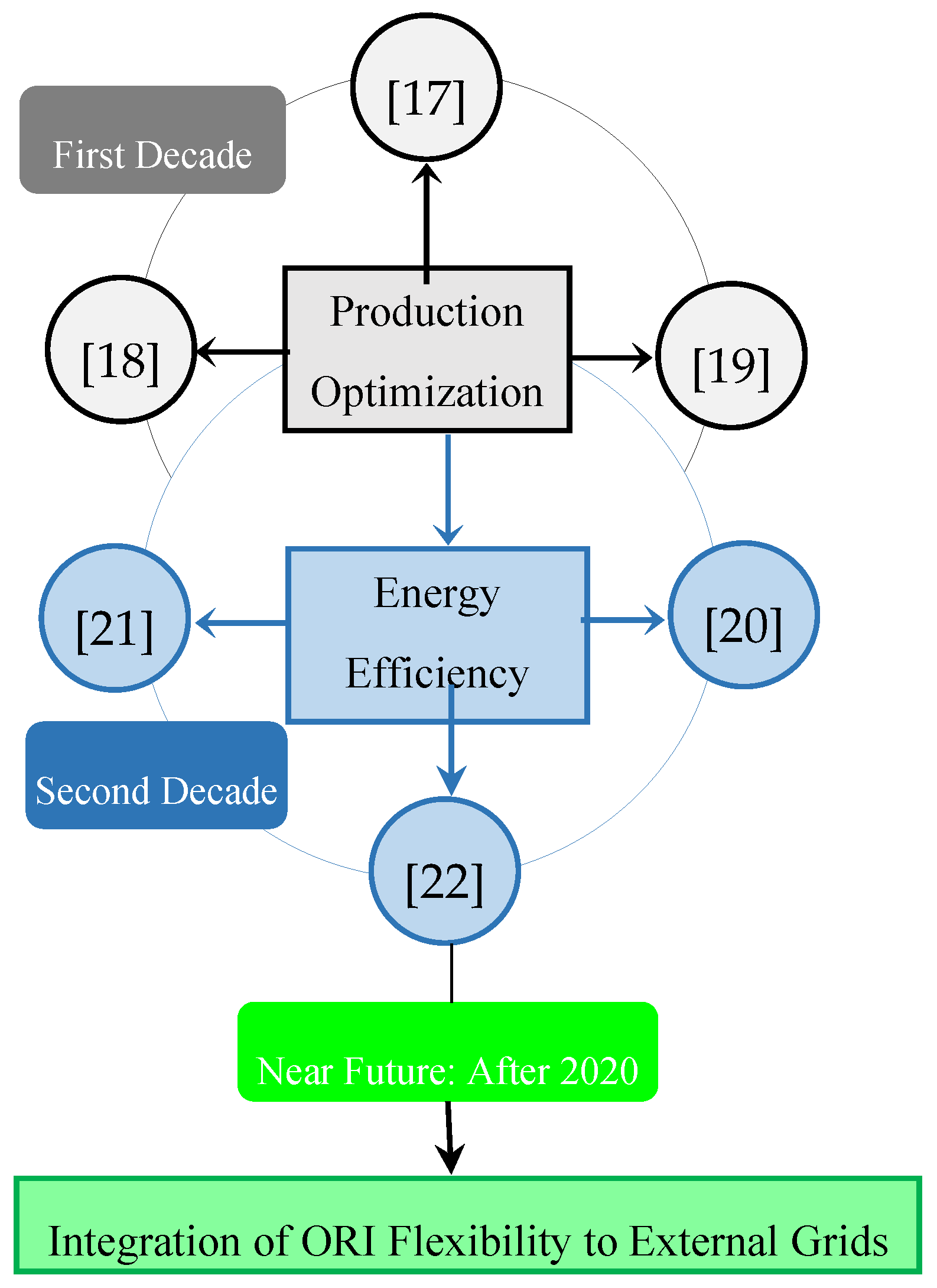
1.3. Paper Contributions and Organization

Based on the literature, the existing gaps in the literature can be stated as follows:

(1)

Mathematical frameworks of joint heat-power management in the ORI.

(2)

Integration of ORI flexibility into uncertain electricity markets.

Against the background, this paper proposes a flow-based mathematical model for the whole refining processes of the ORI to investigate the demand flexibilities among the whole processing units. In this way, the mass storage tanks are modeled mathematically between different stages of the refinery processes to store the input mass for a specific time, before being transported to the next refinery unit for further processing. The storage tanks make it possible to provide industrial flexibility to an external network without needing to interrupt or delay the start for upstream processing units. Moreover, the energy consumption of the processing units is described as a function of mass flow instead of fixed consumption. This issue was ignored in previous studies, while playing a crucial role in providing demand flexibility. Besides, to schedule the demand-side flexibility of the industry in an uncertain electricity market, the energy management of the ORI is optimized under electricity price uncertainty. Finally, the robust operation strategies of the ORI are determined in the worst-case realization of the electricity price uncertainty using a robust optimization approach. All in all, the contributions of the problem can be stated as follows:

(1)

Proposing a mathematical framework for whole processing units of the ORI.

(2)

Integrating joint heat-power flexibility of the ORI into the power system under electricity price uncertainty.

(3)

Investigating the role of self-generation facilities and storages on the ORI flexibility potentials.

The rest of the paper is organized as follows. In Section 2, the main industrial processes of a typical ORI plant are explained. In Section 3, the industrial processes of the ORIO are modeled mathematically. Section 4 describes the co-generation facilities of the industry. In Section 5, the mathematical formulation of an industrial boiler is illustrated. In Section 6, the framework of energy cost optimization is explained. The time framework of the industrial processes is described in Section 7. In Section 8, the solution methodology, as well as the robust optimization approach, are stated. Section 9 illustrates the integration of the demand-side flexibility to the external grid qualitatively. In Section 10, the simulation results are stated and discussed. Finally, Section 11 concludes the study.

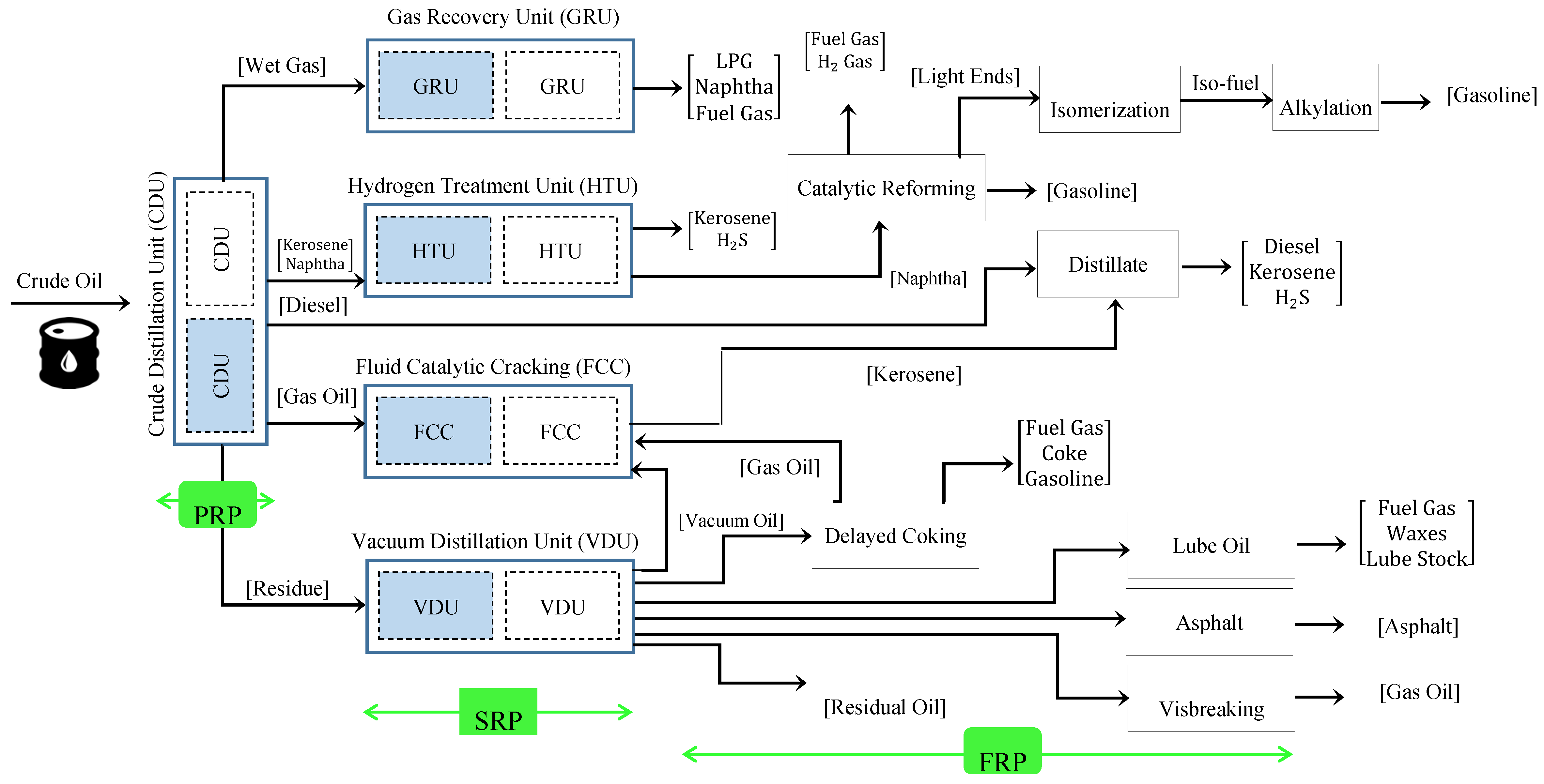
2. Description of Refinery Processes

In this section, the working procedures of a typical oil refinery industry are described briefly. In this paper, the study aims to explore the possibilities of demand-side flexibility among different refining processes of an ORI. To achieve the aim, the whole refining processes are split into three main sections, as follows:

(1)

Section 1: Primary refining processes (PRP), including the crude distillation unit (CDU).

(2)

Section 2: Secondary refining processes (SRP), including the gas recovery unit (GRU), hydrogen treatment unit (HTU), fluid catalytic cracking (FCC), and vacuum distillation unit (VDU).

(3)

Section 3: Final refining processes (FRP), including catalytic reforming unit (CRU), distillate hydroforming unit (DHU), delayed coking unit (DCU), lube oil processing unit (LPU), asphalt processing unit (APU) and visbreaking.

In the first stage, i.e., PRP, the crude oil is transferred to CDU, as a fractioning column, to be heated at about 400 °C. The crude oil, which is a combination of various hydrocarbons, is fractionated to refined products. i.e., wet gas, kerosene, naphtha, diesel, gas oil, and residual fractions. The output flows are cooler and less-volatile components, progressively condensing to liquids. The output products are entered into Section 2, i.e., SRP, for further refining.

The second stage, i.e., SRP, comprises four main refining units. First of all, the wet gas is processed in the GRU, to be split into liquefied petroleum gas (LPG), naphtha, and fuel gas. In the HTU, the kerosene and naphtha are hydrotreated to meet clean fuel requirements [23]. In the third process, the FCC converts the high-boiling, high-molecular-weight hydrocarbon fractions of crude oils, i.e., heavy oil gas, into more valuable gasoline and other products. The FCC is one of the most important refining processes used in an ORI. Finally, the VDU processes the atmospheric residue from the CDU to produce three or four waxy distillate side cuts.

In the third stage, i.e., FRP, the output productions of the SRP are further processed to be converted into marketable petroleum products. In this stage, the CRU is a chemical process used to convert petroleum refinery naphtha distilled from HTU into high-octane liquid products, e.g., gasoline. In this unit, two sub-processes including isomerization and alkylation are performed to enrich the naphtha. In the DHU, the feedstock, i.e., diesel and kerosene, is processed to reduce the Sulphur content. In this unit, the H₂S is produced in addition to the diesel and kerosene. In this stage, DCU, LPU, APU, and visbreaking are four sub-processes which are supplied from the VDU. First of all, the DCU heats the residual oil feed up to its thermal cracking temperature in a furnace with multiple parallel passes. This unit fractionates the heavy, long-chain hydrocarbon molecules of the residual oil into fuel gas, coke, and gasoline [3]. Secondly, the LPU is the final hydrofinishing step to remove the aromatic content and wax. This unit improves the product’s physicochemical properties to meet the color and stability requirements. Fuel gas, waxes, and lube oil are the marketable productions of this unit. Thirdly, the APU processes the asphalt stock to produce high-quality asphalt for roadstone coating objectives. Finally, visbreaking is a processing unit whose aim is to reduce the quantity of residual oil to increase the yield of more valuable middle distillates, e.g., gas oil. Heating in a furnace, the large hydrocarbon molecules are fractionated to small quantities of light hydrocarbons with lower viscosity.

In this section, the main refining units of the ORI is illustrated briefly. Detailed descriptions of the refining units are not within the scope of this study. The enthusiastic readers are encouraged to study book [3] for further clarifications. In the next sections, the proposed structure of the refining procedures is formulated mathematically.

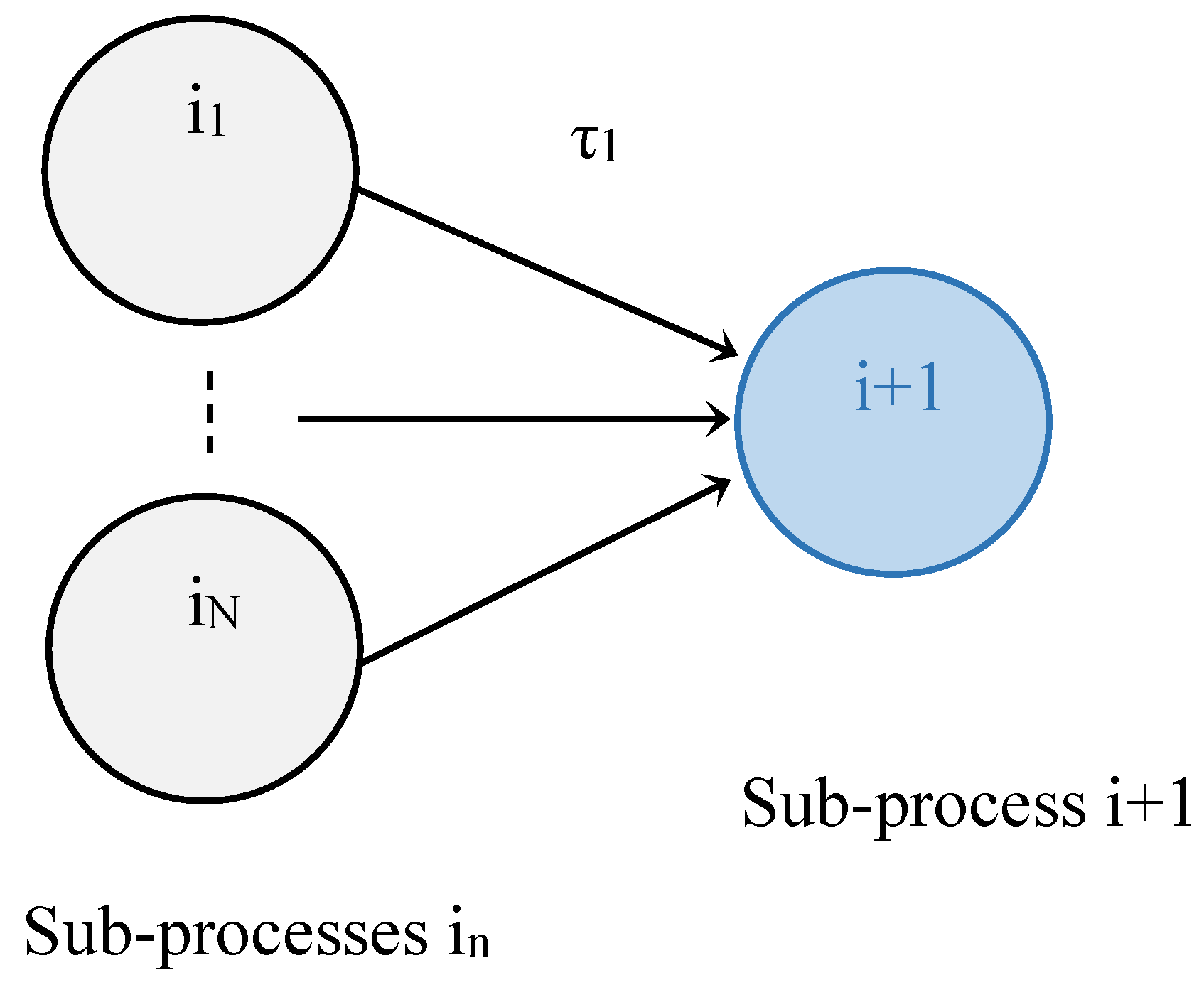
3. Formulation of Oil Refinery Industry

In this section, the refining processes of the ORI are formulated mathematically. To achieve the aim, the PRP and SRP are formulized individually. Regarding the FRP, while the FRP’s procedures depend heavily on the SRP operation, it is assumed that the FRP is operated continuously, receiving feedstock from the SRP. Therefore, the mathematical formulations and operational constraints of FRP are ignored, to avoid increasing complexity and intractability.

First of all, the mathematical structure of the PRP is modeled as follows:

$${\mathsf{\Pi }}_{\mathrm{t}}^{\mathrm{CDU}}{=\mathsf{\Pi }}_{\mathrm{R}}^{\mathrm{CDU}}{\times \mathrm{X}}_{\mathrm{t}}^{\mathrm{CDU}}$$

(1)

$${\mathsf{\Lambda }}_{\mathrm{t}}^{\mathrm{CDU}}={\mathsf{\Lambda }}_{\mathrm{R}}^{\mathrm{CDU}}\times {\mathrm{X}}_{\mathrm{t}}^{\mathrm{CDU}}$$

(2)

$${\mathrm{X}}_{\mathrm{t}}^{\mathrm{CDU}}={\mathsf{\eta }}^{\mathrm{PRP}}\times {\mathrm{X}}_{\mathrm{t}}^{\mathrm{SRP}}$$

(3)

$${\mathrm{SoS}}_{\mathrm{t}}^{\mathrm{CDU}}={\mathrm{SoS}}_{\mathrm{t}-1}^{\mathrm{CDU}}+{\mathrm{X}}_{\mathrm{t},\mathrm{in}}^{\mathrm{CDU}}-{\mathrm{X}}_{\mathrm{t},\mathrm{out}}^{\mathrm{CDU}}$$

(4)

$${\mathrm{X}}_{\mathrm{t},\mathrm{in}}^{\mathrm{CDU}}={\mathrm{X}}_{\mathrm{t}}^{\mathrm{CDU}}$$

(5)

$${\mathrm{X}}_{\mathrm{t},\mathrm{out}}^{\mathrm{CDU}}={\mathrm{X}}_{\mathrm{t}}^{\mathrm{SRP}}$$

(6)

In this model, Equations (1) and (2) illustrate the electricity and heat consumption of CDU as a function of variable material flow, respectively. Equation (3) describes the relationship between input and output material flows of PRP and SRP. Equation (4) shows the state of storage (SoS) for the CDU. In this way, the SoS depends on the previous SoS, input, and output material flows. Equality (5) states that the input flow of the storage is supplied from CDU. Besides, Equality (6) expresses that the output flow from the storage supplies the SRP unit.

The mathematical model of PRP, i.e., Equations (1)–(6), is subject to the following constraints:

$${\mathrm{X}}_{\min }^{\mathrm{CDU}}\le {\mathrm{X}}_{\mathrm{t}}^{\mathrm{CDU}}\le {\mathrm{X}}_{\max }^{\mathrm{CDU}}$$

(7)

$${\mathsf{\Pi }}_{\min }^{\mathrm{CDU}}\le {\mathsf{\Pi }}_{\mathrm{t}}^{\mathrm{CDU}}\le {\mathsf{\Pi }}_{\max }^{\mathrm{CDU}}$$

(8)

$${\mathsf{\Lambda }}_{\min }^{\mathrm{CDU}}\le {\mathsf{\Lambda }}_{\mathrm{t}}^{\mathrm{CDU}}\le {\mathsf{\Lambda }}_{\max }^{\mathrm{CDU}}$$

(9)

$${\mathrm{SoS}}_{\min }^{\mathrm{CDU}}\le {\mathrm{SoS}}_{\mathrm{t}}^{\mathrm{CDU}}\le {\mathrm{SoS}}_{\max }^{\mathrm{CDU}}$$

(10)

Inequality (7) limits the material flow of CDU between lower and upper thresholds. While the electricity and heat consumptions of the CDU depend on the variable material flow, Equations (8) and (9) bound the variations of the electricity and heat consumptions, respectively. Inequality (10) limits the storage capacity of the CDU.

The PRP unit is comprised of one unit, i.e., CDU. The output material of the CDU supplies the SRP unit, which includes four refinery processes. Based on the abovementioned facts, the mathematical formulations of the SRP can be presented as follows:

$$\forall \mathrm{i}\in \{\mathsf{\Theta }\}=\{\mathrm{GRU},\mathrm{HTU},\mathrm{FCC},\mathrm{VDU}\}:|\begin{array}{c}{\mathsf{\Pi }}_{\mathrm{t}}^{\mathrm{SRP}}={\displaystyle \sum _{\mathrm{i}\in \left\{\mathsf{\Theta }\right\}}^{}{\mathsf{\Pi }}_{\mathrm{t}}^{\mathrm{i}}}\\ {\mathsf{\Lambda }}_{\mathrm{t}}^{\mathrm{SRP}}={\displaystyle \sum _{\mathrm{i}\in \left\{\mathsf{\Theta }\right\}}^{}{\mathsf{\Lambda }}_{\mathrm{t}}^{\mathrm{i}}}\end{array}$$

(11)

$$|\begin{array}{c}{\left[{\mathsf{\Pi }}_{\mathrm{t}}^{\mathrm{i}}\right]}_{\mathrm{i}\times 1}{=\mathsf{\Pi }}_{\mathrm{R}}^{\mathrm{i}}{\left[\mathrm{I}\right]}_{\mathrm{i}\times \mathrm{i}}\times {\left[{\mathrm{X}}_{\mathrm{t}}^{\mathrm{i}}\right]}_{\mathrm{i}\times 1}\\ {\left[{\mathsf{\Lambda }}_{\mathrm{t}}^{\mathrm{i}}\right]}_{\mathrm{i}\times 1}={\mathsf{\Lambda }}_{\mathrm{R}}^{\mathrm{i}}{\left[\mathrm{I}\right]}_{\mathrm{i}\times \mathrm{i}}\times {\left[{\mathrm{X}}_{\mathrm{t}}^{\mathrm{i}}\right]}_{\mathrm{i}\times 1}\end{array}$$

(12)

$${\mathrm{X}}_{\mathrm{t}}^{\mathrm{SRP}}={\displaystyle \sum _{\mathrm{i}\in \left\{\mathsf{\Theta }\right\}}^{}{\mathrm{X}}_{\mathrm{t}}^{\mathrm{i}}}$$

(13)

$${\left[{\mathrm{SoS}}_{\mathrm{t}}^{\mathrm{i}}\right]}_{\mathrm{i}\times 1}={\left[{\mathrm{SoS}}_{\mathrm{t}-1}^{\mathrm{i}}\right]}_{\mathrm{i}\times 1}+{\left[{\mathrm{X}}_{\mathrm{t},\mathrm{in}}^{\mathrm{i}}\right]}_{\mathrm{i}\times 1}-{\left[{\mathrm{X}}_{\mathrm{t},\mathrm{out}}^{\mathrm{i}}\right]}_{\mathrm{i}\times 1}$$

(14)

$${\mathrm{X}}_{\mathrm{t},\mathrm{in}}^{\mathrm{i}}={\mathsf{\rho }}^{\mathrm{i}}\times {\mathrm{X}}_{\mathrm{t}}^{\mathrm{SRP}}$$

(15)

In this model, Equation (11) describes the total electricity and heat consumption of SRP as the summation of demand of i refinery units. Equation (12) states the electricity and heat consumptions of i refinery units as the function of variable material flow in a matrix form. Note that [I]_i×i is an identity matrix, which is the i × i square matrix with ones on the main diagonal and zeros elsewhere. Equality (13) ensures the material flow balance in the SRP units. In this way, the total input flow to the SRP must be equal to the summation of input flows to i refinery units. Equation (14) states the SoS for i units of SRP in the matrix form. In this way, the input flow of storage for subprocess i is a fraction of total material flow to the SRP. This constraint is expressed by Equation (15).

Following a similar pattern, the mathematical model of SRP, i.e., (11)–(15), must meet the following constraints:

$${\left[{\mathrm{X}}_{\min }^{\mathrm{i}}\right]}_{\mathrm{i}\times 1}\le {\left[{\mathrm{X}}_{\mathrm{t}}^{\mathrm{i}}\right]}_{\mathrm{i}\times 1}\le {\left[{\mathrm{X}}_{\max }^{\mathrm{i}}\right]}_{\mathrm{i}\times 1}$$

(16)

$${\left[{\mathsf{\Pi }}_{\min }^{\mathrm{i}}\right]}_{\mathrm{i}\times 1}\le {\left[{\mathsf{\Pi }}_{\mathrm{t}}^{\mathrm{i}}\right]}_{\mathrm{i}\times 1}\le {\left[{\mathsf{\Pi }}_{\max }^{\mathrm{i}}\right]}_{\mathrm{i}\times 1}$$

(17)

$${\left[{\mathsf{\Lambda }}_{\min }^{\mathrm{i}}\right]}_{\mathrm{i}\times 1}\le {\left[{\mathsf{\Lambda }}_{\mathrm{t}}^{\mathrm{i}}\right]}_{\mathrm{i}\times 1}\le {\left[{\mathsf{\Lambda }}_{\max }^{\mathrm{i}}\right]}_{\mathrm{i}\times 1}$$

(18)

$${\left[{\mathrm{SoS}}_{\min }^{\mathrm{i}}\right]}_{\mathrm{i}\times 1}\le {\left[{\mathrm{SoS}}_{\mathrm{t}}^{\mathrm{i}}\right]}_{\mathrm{i}\times 1}\le {\left[{\mathrm{SoS}}_{\max }^{\mathrm{i}}\right]}_{\mathrm{i}\times 1}$$

(19)

$${\displaystyle \sum _{\mathrm{t}=1}^{\mathrm{N}}{\mathrm{X}}_{\mathrm{t}}^{\mathrm{SRP}}}={\mathrm{X}}_{}^{\mathrm{Ord}}$$

(20)

In these constraints, inequalities (16)–(19) determine the lower and upper thresholds for material flow, electricity consumption, heat demand, and storage capacity for refinery subprocesses of the SRP, respectively. Equality (20) ensures that the total production of the ORI meets the total ordered value of the consumers. This is an important constraint that guarantees the industry’s production without interruption or reduction.

Finally, to give a general overview of the refinery processes of the ORI, a schematic diagram is depicted in Figure 2. The basic structure is extracted from [3]. In this figure, the material storages, which are shown in blue boxes, are added to refinery units to increase the demand flexibility of the refinery industry.

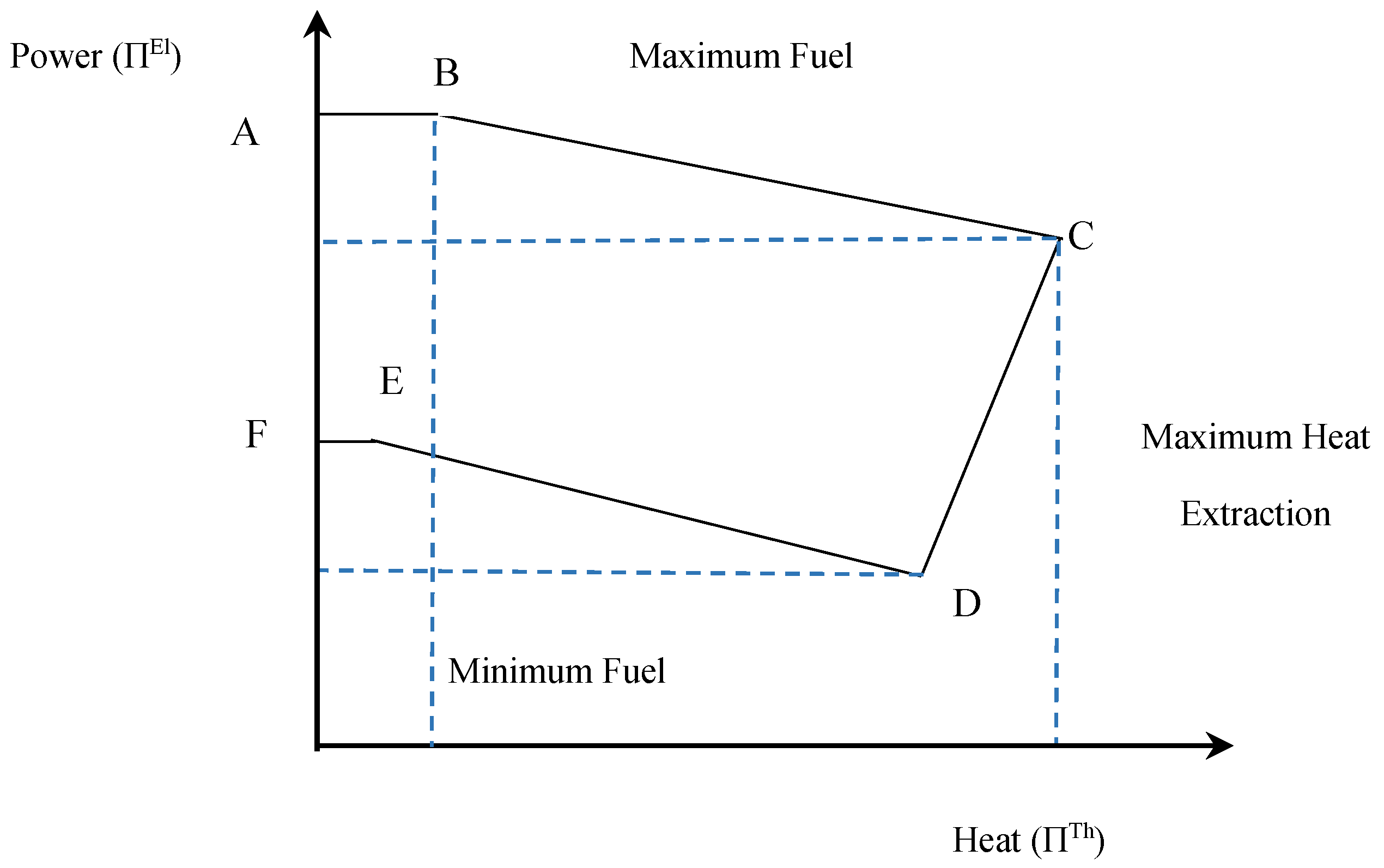
4. Co-Generation Units

The ORI consumes a lot of energy in terms of electricity and heat (steam). Generally, the ORIs are equipped with self-generation facilities to supply the required electricity as a stand-alone grid. In this way, the ORI has a high capacity to supply the power grid during power shortage. Therefore, the ORI can be operated in two modes, including stand-alone and grid-connected. Besides, some refining processes consume a large amount of steam. Broadly, the steam demand of the ORI is supplied by the industrial boilers. However, some parts of steam demand can be supplied by the co-generation units. As a result, power-only units should be substituted by the combined heat and power (CHP) unit. All in all, the mathematical formulations of the CHP units can be stated as follows:

$$\begin{array}{l}{\mathrm{C}}_{\mathrm{t}}^{\mathrm{CHP}}=\left[{\mathsf{\alpha }}_{\mathrm{El}}^{}{+(\mathsf{\beta }}_{\mathrm{El}}^{}{\times \mathsf{\Pi }}_{\mathrm{t}}^{\mathrm{El}}{)+(\mathsf{\gamma }}_{\mathrm{El}}^{}{\times \mathsf{\Pi }}_{\mathrm{t}}^{{\mathrm{El}}^2})\right]\\ +\left[{(\mathsf{\beta }}_{\mathrm{Th}}^{}\times {\mathsf{\Pi }}_{\mathrm{t}}^{\mathrm{Th}}{)+(\mathsf{\gamma }}_{\mathrm{Th}}^{}\times {\mathsf{\Pi }}_{\mathrm{t}}^{{\mathrm{Th}}^2})\right]+\left[{\mathsf{\nu }}_{\mathrm{CHP}}^{}\times {\mathsf{\Pi }}_{\mathrm{t}}^{\mathrm{El}}\times {\mathsf{\Pi }}_{\mathrm{t}}^{\mathrm{Th}}\right]\end{array}$$

(21)

$${\mathrm{G}}_{\mathrm{t}}^{\mathrm{CHP}}=\frac{\left({\mathsf{\Pi }}_{\mathrm{t}}^{\mathrm{El}}{+\mathsf{\Pi }}_{\mathrm{t}}^{\mathrm{Th}}\right)}{{\mathsf{\eta }}^{\mathrm{CHP}}{\times \mathrm{G}}^{\mathrm{HV}}}$$

(22)

Equation (21) shows the cost function of CHP in terms of power and heat generations. Equation (22) illustrates the gas consumption of the CHP as a function of the power-heat generation, by considering the local gas heat value and generation efficiency. The cost function of the CHP, i.e., Equation (21), is subject to the following constraints

$${\mathsf{\Pi }}_{\min }^{\mathrm{El}}({\mathsf{\Pi }}_{\mathrm{t}}^{\mathrm{Th}})\le {\mathsf{\Pi }}_{\mathrm{t}}^{\mathrm{El}}\le {\mathsf{\Pi }}_{\max }^{\mathrm{El}}({\mathsf{\Pi }}_{\mathrm{t}}^{\mathrm{Th}})$$

(23)

$${\mathsf{\Pi }}_{\min }^{\mathrm{Th}}({\mathsf{\Pi }}_{\mathrm{t}}^{\mathrm{El}})\le {\mathsf{\Pi }}_{\mathrm{t}}^{\mathrm{Th}}\le {\mathsf{\Pi }}_{\max }^{\mathrm{Th}}({\mathsf{\Pi }}_{\mathrm{t}}^{\mathrm{El}})$$

(24)

$${\mathsf{\Pi }}_{\mathrm{t}+1}^{\mathrm{El}}-{\mathsf{\Pi }}_{\mathrm{t}}^{\mathrm{El}}\le {\mathrm{R}}_{\mathrm{CHP}}^{\mathrm{U}}$$

(25)

$${\mathsf{\Pi }}_{\mathrm{t}}^{\mathrm{El}}-{\mathsf{\Pi }}_{\mathrm{t}-1}^{\mathrm{El}}\le {\mathrm{R}}_{\mathrm{CHP}}^{\mathrm{D}}$$

(26)

Inequality (23) states that the upper and lower boundaries of electricity generation of the CHP unit are a function of the heat generation of the unit. In the same way, constraint (24) illustrates that the upper and lower boundaries of heat generation of the CHP are a function of the electricity generation. These constraints make the feasible operation range (FOR) of the CHP into a polygon area. The parametric FOR is depicted in Figure 3. Equations (25) and (26) explain the ramp-up/-down of the CHP.

5. Industrial Boiler

The ORIs consume a large amount of steam in the refinery processes. The co-generation units can supply some part of steam demand. However, in many cases, the steam demand is high, and the co-generation units are not able to cope with the full steam demand of the refinery processes. Therefore, industrial boilers are considered to compensate for the lack of steam generation. The cost function of an industrial boiler is described as follows:

$${\mathrm{C}}_{\mathrm{t}}^{\mathrm{Bo}}{=\mathsf{\alpha }}_{\mathrm{Bo}}^{}{+(\mathsf{\beta }}_{\mathrm{Bo}}^{}{\times \mathsf{\Pi }}_{\mathrm{t}}^{\mathrm{Bo}}{)+(\mathsf{\gamma }}_{\mathrm{Bo}}^{}{\times \mathsf{\Pi }}_{\mathrm{t}}^{{\mathrm{Bo}}^2})$$

(27)

$${\mathsf{\Pi }}_{\min }^{\mathrm{Bo}}\le {\mathsf{\Pi }}_{\mathrm{t}}^{\mathrm{Bo}}\le {\mathsf{\Pi }}_{\max }^{\mathrm{Bo}}$$

(28)

Equation (27) shows the cost function of the boiler as a function of heat generation. The heat generation of the boiler is bounded to lower and upper thresholds by inequality (28). Note that α_Bo, β_Bo, and γ_Bo are coefficients of the cost function.

6. Energy Cost Optimization

In this study, the problem aims to optimize the energy consumption/production of the ORI to provide structural flexibility to the external networks, i.e., IEM, meeting the daily ordered value of final production. Therefore, the objective function of the problem can be stated as follows:

$$\mathrm{Minimize}\left(\mathrm{Cos}\mathrm{t}\right)={\displaystyle \sum _{\mathrm{t}=1}^{\mathrm{N}}\left[{\mathrm{C}}_{\mathrm{t}}^{\mathrm{Grid}}+{\mathrm{C}}_{\mathrm{t}}^{\mathrm{CHP}}{+\mathrm{C}}_{\mathrm{t}}^{\mathrm{Bo}}\right]}$$

(29)

$${\mathrm{C}}_{\mathrm{t}}^{\mathrm{Grid}}{=(\mathsf{\Pi }}_{\mathrm{t}}^{\mathrm{Grid}}{\times \mathsf{\lambda }}_{\mathrm{t}}^{\mathrm{Grid}})$$

(30)

Equation (29) illustrates that the objective function of the problem is to minimize the operation cost of the ORI. The objective function is comprised of three terms. The first term is the procurement cost from the power grid. The second term shows the cost function of the CHP unit which was modeled in (21)–(26). The third term states the cost function of the industrial boiler which was formulized in (27) and (28). Equation (30) explains the procurement cost from the power grid. In this way, the ORI can sell the excess of generated electricity to the main grid (Π^Grid < 0) or purchase the deficit of power from the network (Π^Grid > 0).

In addition to the operational constraints of the refinery processes, CHP unit and industrial boiler, i.e., Equations (1)–(28), the energy management of the ORI is subject to the following constraints:

$${\mathsf{\Pi }}_{\mathrm{t}}^{\mathrm{ED}}={\mathsf{\Pi }}_{\mathrm{t}}^{\mathrm{Grid}}+{\mathsf{\Pi }}_{\mathrm{t}}^{\mathrm{El}}$$

(31)

$${\mathsf{\Pi }}_{\mathrm{t}}^{\mathrm{ED}}={\mathsf{\Pi }}_{\mathrm{t}}^{\mathrm{CDU}}+{\mathsf{\Pi }}_{\mathrm{t}}^{\mathrm{SRP}}$$

(32)

$${\mathsf{\Lambda }}_{\mathrm{t}}^{\mathrm{SD}}={\mathsf{\Lambda }}_{\mathrm{t}}^{\mathrm{Bo}}+{\mathsf{\Lambda }}_{\mathrm{t}}^{\mathrm{Th}}$$

(33)

$${\mathsf{\Lambda }}_{\mathrm{t}}^{\mathrm{SD}}={\mathsf{\Lambda }}_{\mathrm{t}}^{\mathrm{CDU}}+{\mathsf{\Lambda }}_{\mathrm{t}}^{\mathrm{SRP}}$$

(34)

$${\mathsf{\Lambda }}_{\mathrm{t}}^{\mathrm{Bo}}=\kappa \times {\mathsf{\Pi }}_{\mathrm{t}}^{\mathrm{Bo}}$$

(35)

$${\mathsf{\Lambda }}_{\mathrm{t}}^{\mathrm{Th}}=\kappa \times {\mathsf{\Pi }}_{\mathrm{t}}^{\mathrm{Th}}$$

(36)

$${-\mathsf{\Pi }}_{\max }^{\mathrm{El}}\le {\mathsf{\Pi }}_{\mathrm{t}}^{\mathrm{Grid}}\le {\mathsf{\Pi }}_{\mathrm{Max}}^{\mathrm{ED}}$$

(37)

Equation (31) illustrates the electrical demand balance of the ORI, which is the summation of power procurement from the grid and power generation of the CHP. On the other hand, Equation (32) shows that the total electricity consumption of the ORI is equal to the electrical demand of PRP plus the electrical demand of SRP. Following a similar pattern, Equation (33) expresses that the total steam demand of the ORI is the summation of the steam generation of the CHP and the boiler. From the demand side, Equation (34) describes the total demand of the ORI as the summation of steam demand in PRP and SRP. Total thermal energy needed to generate steam in boiler and CHP is illustrated by Equations (35) and (36), respectively.

Finally, Equation (37) describes the upper and lower thresholds of transactive power. In detail, the inequality states that the upper bound of traded power, i.e., purchased power from the main grid Π^Grid > 0, is equal to the nominal electrical demand of the ORI. Besides, the lower bound of traded power, i.e., sold power to the main grid Π^Grid < 0, is equal to the maximum electricity generation capacity of the CHP.

7. Time Framework

Generally, energy management problems are considered based on hourly time slots. In the industrial sector, many research studies optimized the operational processes of heavy industries, e.g., cement plants and metal smelting factories, on an hourly basis. In the industries with low interdependency between industrial sub-processes, the hourly basis is a practical time framework to avoid increasing complexity in modeling. In contrast, in the industries with high interdependency, the hourly basis may fail to optimize the industrial processes effectively. In this regard, if a heavy interdependency is considered between refinery processes in the ORI, the time framework of the problem should be split into sub-hourly time slots. To address the sub-hourly time framework, an operation flow graph is developed in this study in accordance with [15].

Figure 4 describes the schematic diagram for the operation flow graph of two consecutive refinery stages.

To elaborate the procedure, suppose that the refinery process i+1 is supplied by the refinery sub-processes i₁, i₂, …, i_N. Because the process i+1 receives the raw materials from N refinery sub-processes, the operation of the process i may start only if the operations of sub-processes i₁, i₂, …, i_N are finished. The parameter τ_n is the weighting factor multiplied by the sub-hourly time slot. For example, the operational process to supply process i + 1 with sub-process i₁ takes τ₁ × T_m time. Therefore, the start-up time of sub-process i + 1 is described as follows:

$${\mathrm{t}}_{(\mathrm{i}+1)}^{\mathrm{start}}={\displaystyle \sum _{\mathrm{n}=1}^{\mathrm{N}}{\mathsf{\tau }}_{\mathrm{n}}{\times \mathrm{T}}_{\mathrm{m}}}$$

(38)

Note that T_m is the sub-hourly time slot (minute). Moreover, it is assumed that the refinery sub-processes i₁, i₂, …, i_N are not concurrent. In contrast, if two processes are performed concurrently, the biggest processing time is replaced in Equation (38). There is the same pattern for more than two concurrent sub-processes.

8. Solution Methodology

In this study, the ORI can purchase/sell the deficit/excess of electrical energy from/to the power network, i.e., the wholesale electricity market. Generally, the electricity price of the wholesale market is a variable with imperfect data [25]. Therefore, the problem is under electricity price uncertainty. Addressing the electricity price as a stochastic variable, a non-deterministic approach is adopted to solve the program. To achieve the aim, a robust optimization approach is used as the solution methodology. In the next subsections, first of all, the electricity price is modeled and uncertainty bound. Afterwards, an iterative procedure is used to determine the robust strategies of the ORI against the uncertain electricity price. The robust strategies mean the optimized strategies in the worst-case realization of the electricity price uncertainty.

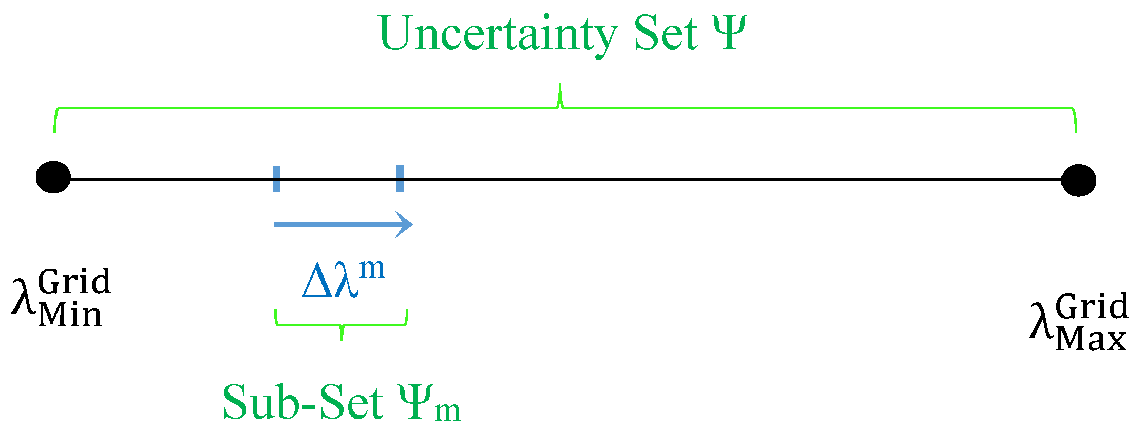
8.1. Electricity Price Uncertainty

In this study, the problem aims to co-optimize the joint electricity-heat procurement under electricity price uncertainty. The ORI can be connected to the main grid to compensate for the lack of electricity when the power system faces a power shortage or negative power imbalance. In contrast, the ORI prefers to purchase power from the main grid when the power system experiences the power excess or positive imbalance. In the former, the electricity price is high; therefore, the ORI should procure the required energy from the self-generation facilities as much as possible. Moreover, the excess power generation can be injected into the power system to help the power system making the load balance. Adversely, in the latter, the electricity price is low. In such s situation, the ORI may prefer to shut the self-generation facilities down to be supplied from the main grid. Making a decision about the generation unit commitment, the electricity price plays a crucial role. While the electricity price is a stochastic variable with imperfect data, the applicable studies should address the price uncertainties in the electricity market. In this study, to incorporate the electricity price uncertainty into the program, an envelope bound is considered for the electricity price uncertainty. The envelope bound is modeled as follows [26]:

$$\mathsf{\Psi }=\left[{\mathsf{\lambda }}_{\mathrm{Min}}^{\mathrm{Grid}},{\mathsf{\lambda }}_{\mathrm{Max}}^{\mathrm{Grid}}\right]=\left[(1-\mathsf{\delta })\times {\tilde{\mathsf{\lambda }}}_{\mathrm{t}}^{\mathrm{Grid}},(1+\mathsf{\delta })\times {\tilde{\mathsf{\lambda }}}_{\mathrm{t}}^{\mathrm{Grid}}\right]$$

(39)

Equality (39) determines a robustness region Ψ for the uncertain electricity price with lower and upper thresholds. The electricity price can take values within the whole interval Ψ. Therefore, to determine the robust strategies under possible realizations of the electricity price, the robustness region is portioned into M subintervals. This procedure can be stated as follows [27]:

$${\mathsf{\Psi }}_{\mathrm{m}}=\left\{{\mathsf{\lambda }}_{\mathrm{t}}^{\mathrm{Grid}}\in ℝ\begin{array}{cc},& \begin{array}{l}\begin{array}{cc}\forall \mathrm{t}=1,\dots ,\mathrm{N}:& {\mathsf{\lambda }}_{\mathrm{t}}^{\mathrm{M}}\in \left[{\mathsf{\lambda }}_{\mathrm{Min}}^{\mathrm{Grid}}{,\mathsf{\lambda }}_{\mathrm{Min}}^{\mathrm{Grid}}{+\mathsf{\Delta }\mathsf{\lambda }}^{\mathrm{m}}\right]\end{array}\\ \begin{array}{cc}\forall \mathrm{m}=1,\dots ,\mathrm{M}:& {\mathsf{\Delta }\mathsf{\lambda }}^{\mathrm{m}}=\mathrm{m}\times \frac{\left|{\mathsf{\lambda }}^{\max }{-\mathsf{\lambda }}^{\min }\right|}{\mathrm{M}}\end{array}\end{array}\end{array}\right\}$$

(40)

Equation (40) portions the robustness region Ψ into m = 1, …, M subintervals, i.e., Ψ_m. Therefore, the problem can be optimized in m subintervals of the electricity price uncertainty, instead of lower and upper bounds. Note that m = {1, …, M} is a counter index to cover the whole interval of the uncertainty set Ψ. Figure 5 illustrates the envelope bound for the electricity price uncertainty.

8.2. Robust Optimization Approach

Based on the abovementioned facts, the problem aims to determine the robust strategies of the ORI in the wholesale electricity market with price uncertainty. Therefore, the problem optimizes the operational strategies under the worst-case realization of the electricity price uncertainty. As a result, the objective function of the problem, i.e., (29), is restated as follows:

$$\mathrm{Minimize}\left(\mathrm{Cos}\mathrm{t}\right)={\displaystyle \sum _{\mathrm{t}=1}^{\mathrm{N}}\left[\mathrm{Maximum}\left(C_t^{\mathrm{Grid}}\right){+\mathrm{C}}_{\mathrm{t}}^{\mathrm{CHP}}{+\mathrm{C}}_{\mathrm{t}}^{\mathrm{Bo}}\right]}$$

(41)

To solve the problem, by using the duality theorem, the primal min-max problem is converted to a dual robust mixed-integer quadratic program (R-MIQP) as follows:

$$\mathrm{Minimize}\left(\mathrm{Cos}\mathrm{t}\right)={\displaystyle \sum _{\mathrm{t}=1}^{\mathrm{N}}\left[{\mathrm{C}}_{\mathrm{t}}^{\mathrm{Grid}}{+\mathrm{C}}_{\mathrm{t}}^{\mathrm{CHP}}{+\mathrm{C}}_{\mathrm{t}}^{\mathrm{Bo}}\right]}+{\displaystyle \sum _{\mathrm{t}=1}^N{\mathsf{\xi }}_{\mathrm{t}}}+\mathsf{\Gamma }\mathsf{\psi }$$

(42)

$$\begin{array}{cc}\forall \mathrm{t}\in \mathrm{N},\forall {\mathsf{\xi }}_t\ge 0,\forall \mathsf{\psi }\ge 0:& {\mathsf{\xi }}_{\mathrm{t}}+\mathsf{\psi }\ge ({\tilde{\mathsf{\lambda }}}_{\mathrm{t}}^{\mathrm{Grid}}\times {\mathsf{\Pi }}_{\mathrm{t}}^{\mathrm{Grid}})\end{array}$$

(43)

Equation (42) presents the final R-MIOP, which is solved to determine optimized strategies. Inequality (43) describes symbols ξ_t and ψ_t as dual variables of corresponding constraints in the duality theorem. In order to incorporate the uncertainty set Ψ_m into the R-MIQP, the step-by-step algorithm is illustrated in Algorithm 1.

Algorithm 1: Incorporation of robustness region to R-MIQP
1	Investigate lower and upper thresholds of possible electricity price $\to { \mathsf{\lambda }}_{\mathrm{Min}}^{\mathrm{Grid}} \mathrm{and} {\mathsf{\lambda }}_{\mathrm{Max}}^{\mathrm{Grid}}$
2	Construct the envelope bound $\to \mathsf{\Psi } = \left[{\mathsf{\lambda }}_{\mathrm{Min}}^{\mathrm{Grid}},{\mathsf{\lambda }}_{\mathrm{Max}}^{\mathrm{Grid}}\right]$
3	For m = 1, 2, …, M:
4	Add the incremental value $\mathsf{\Delta }{\mathsf{\lambda }}^{\mathrm{m}} \mathrm{to} {\mathsf{\lambda }}_{\mathrm{Min}}^{\mathrm{Grid}} \mathrm{to} \mathrm{construct} {\mathsf{\lambda }}_{\mathrm{t}}^{\mathrm{M}}$
5	Solve R-MIQP Equation (42)
6	Determine robust decisions in worst-case realization of ${\mathsf{\lambda }}_{\mathrm{t}}^{\mathrm{M}}$.
7	Increase counter index m→m + 1
8	End For

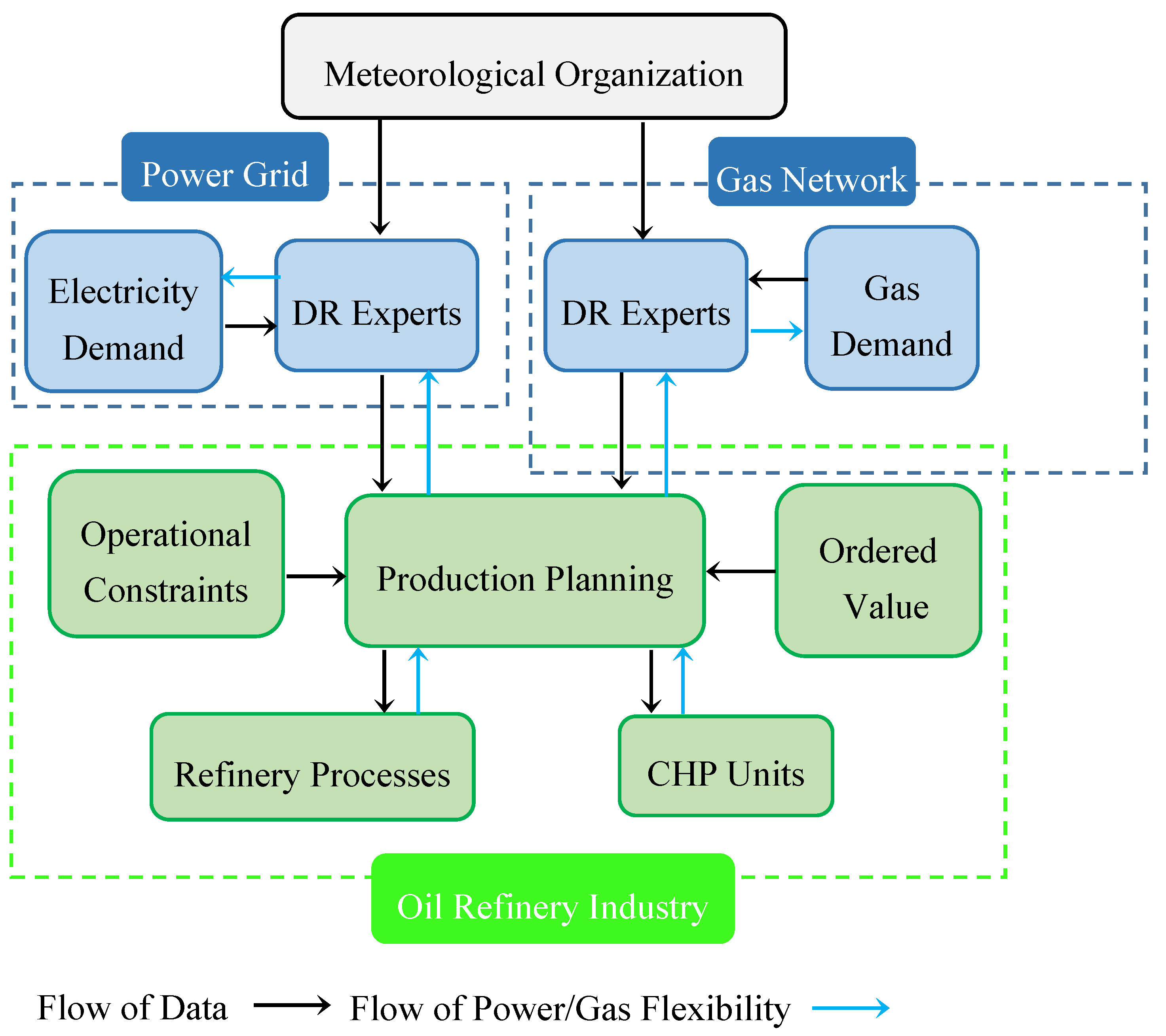
9. Integration of Flexibility to External Networks

As illustrated in the previous sections, the main aim of this study is to use the flexibility potentials of the ORI to overcome the external grid’s limitation. Therefore, the operation of refinery processes is optimized to provide electricity regulation to the power network when a serious electricity shortage occurs or the grid reliability is jeopardized [28]. This issue is a major problem for Iran Energy Market. The Iran Power Grid suffers from a power shortage at hot midday hours of summer, i.e., July to September, when the electrical demand of air conditioning systems of residential and commercial sectors is high. Increasing the capacity of electricity generation and transmission is not an economic decision. The reason is that more than half the capacity of the electricity network is not used out of peak season. Therefore, the practical solution is to optimize the operational processes of industries that consume electricity simultaneously. In this way, the industries equipped with CHP units are satisfactory solutions.

To meet the power limitations of the external grids, the production planning department of the ORI needs to work closely with demand response experts at Iran Power Grid. Based on the weather forecasting received from Iran Meteorological Organization, the demand response experts at Iran Power Grid calculate how much demand flexibility is needed to prevent a power shortage. The amount of demand flexibility is sent to the Production Planning Department of the ORI to optimize the operational processes of the industry for the next 24 h. The production planning department makes the final decision for the operation of the ORI, meeting the industry operational requirements. In this way, minor/daily maintenance programs, crew constraints, daily/weekly ordered value of final productions, and cost data of self-generation facilities are the key factors affecting the final production schedule. In this way, the production planning department can schedule minor maintenance actions to coincide with the peak demand of the external network. These kinds of coordination help the external network to supply demand without interruption.

Figure 6 clarifies the suggested coordination between Iran Power Grid, Meteorological Organization, and Production Planning Department.

To sum up the problem, Figure 7 illustrates the general structure of the proposed approach.

10. Numerical Studies

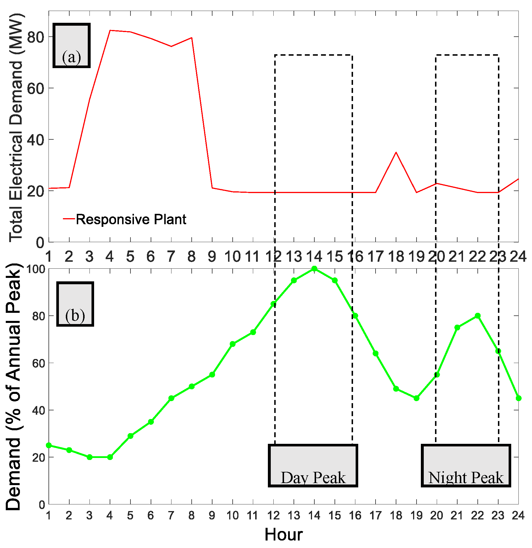
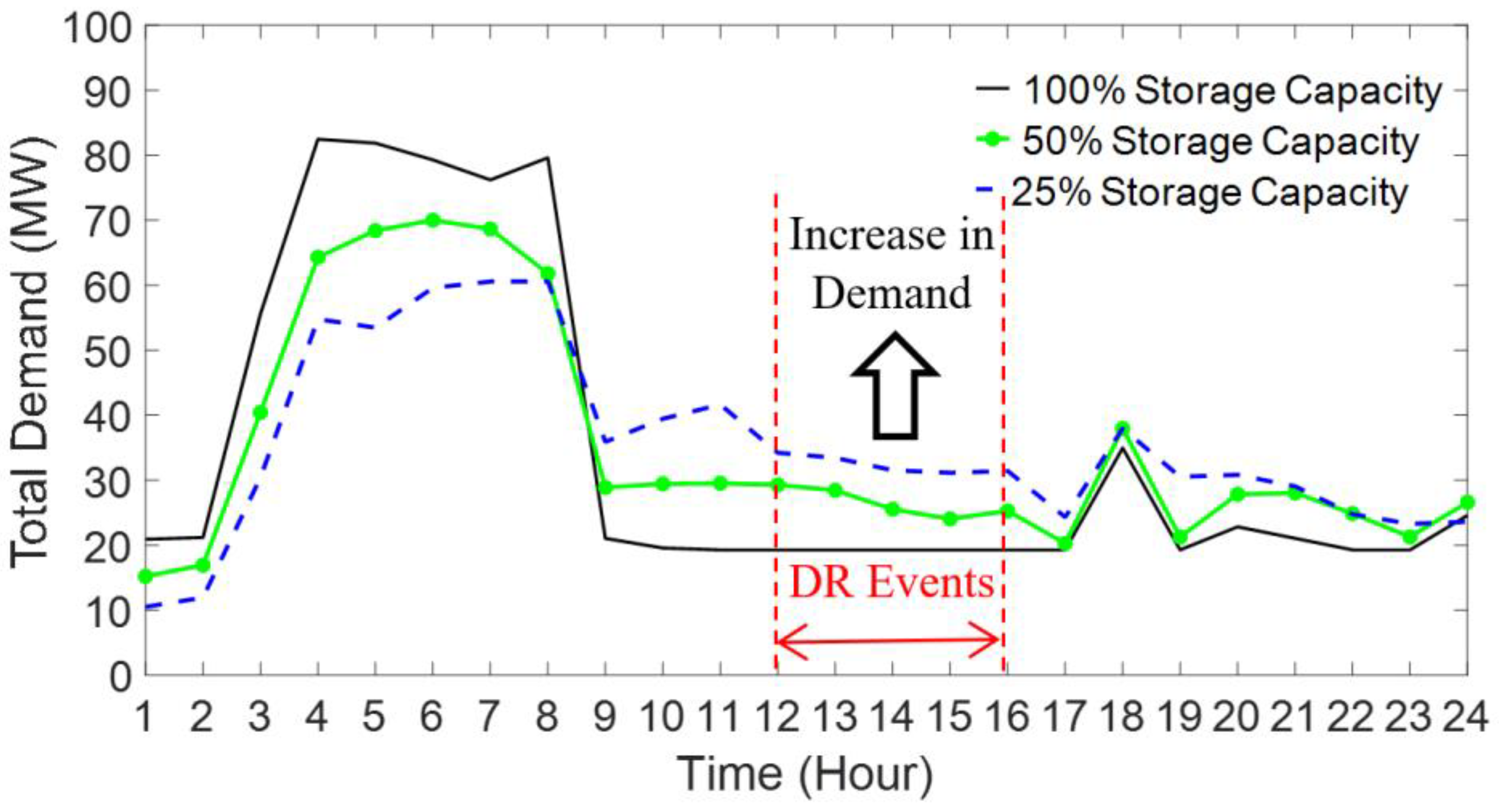
In this section, the proposed approach is implemented in the case studies. In this way, first of all, the input data are illustrated. Afterwards, the simulation results are described and discussed.

10.1. Input Data

The problem is simulated in an ORI to minimize the cost of energy consumption as well as maximize demand flexibility to the IEM. The study horizon is one day, i.e., 24 h. The problem is optimized based on hourly time resolution; therefore, T_m is chosen as 60 min.

The problem aims to determine optimized operation strategies of the ORI in the next 24 h, considering the uncertainty associated with the electricity market price. The target day is a hot day of summer when the IEM suffers from peak electricity demand due to the high electricity consumption of residential and commercial cooling systems. Therefore, the operation of the ORI is optimized to provide flexibility to the IEM in critical hours of both day and night peak hours. It is worth mentioning that the IEM has two peak durations a day in the summer. The first is the day peak that occurs between hours 12 and 16. The second is called the night peak during hours 21 to 23. The former stems from the high electrical demand of cooling systems, while the latter is caused by the high demand of lighting systems. Therefore, the demand-side flexibility of Iranian industries, especially the ORI, should be scheduled to provide power flexibility to the IEM in both day and night peak hours.

The pilot plant is a test ORI, called Pars ORI, in the south-west of Iran, where huge numbers of oil refinery plants are located in one of the most oil-rich areas in the world [29]. The total refinery capacity of the ORI is 48,000 ton/day crude oil. The scheduled vale of oil refinery is supposed to be 44,000 tons on the target day.

Table 1. Technical characteristics of the pilot Pars ORI.

Sub-Process	Electrical Demand (MWh/kt)	Steam Demand (GJ/kt)	Storage Capacity (kt)	Threshold of Feedstock Flow (kt/h)
CDU	3.68	8	4	1~4
GRU	7.5	12	2	0.25~1
HTU	20.5	33	2	0.25~1
FCC	25	25	2	0.25~1
VDU	18	138	2	0.25~1

describes the technical characteristics of the Pars ORI. Besides,

Table 2. Technical data of CHP and industrial boiler.

CHP	Cost Function Equation (21)	αEl	βEl	γEl	βTh	γTh	νCHP
		2950	28.5	0.1045	4.2	0.03	0.031
	FOR (ΠEl, ΠTh) Figure 3	A	B	C	D	E	F
		(247,0)	(247,0)	(215,180)	(81,104.8)	(98.8,0)	(98.8,0)
Boiler	Cost Function Equation (27)	αBo	βBo	γBo	${\mathsf{\Pi }}_{\min }^{\mathrm{Bo}}$	${\mathsf{\Pi }}_{\max }^{\mathrm{Bo}}$
		0	14.7	0	1	85

illustrates the technical data of CHP and industrial boiler of Pars ORI.

Figure 8 describes the electricity price of the target day of the IEM in June 2017 [30]. In this figure, the upper and lower thresholds of the electricity price are shown. The electricity price is quantified within the area filled by the shadowed area. As the figure reveals, the price gap is divided into 25 intervals to optimize the operation strategies of the ORI in the worst-case realization of the electricity price.

The suggested approach is mathematically modeled in GAMS 24.1.3 [31], linked with MATLAB 2019R through gdx file interface [20]. To optimize the mathematical formulations, CPLEX [32] and CONOPT solvers [33] are used. The program is simulated in Intel-based computer hardware with 16 GB of RAM.

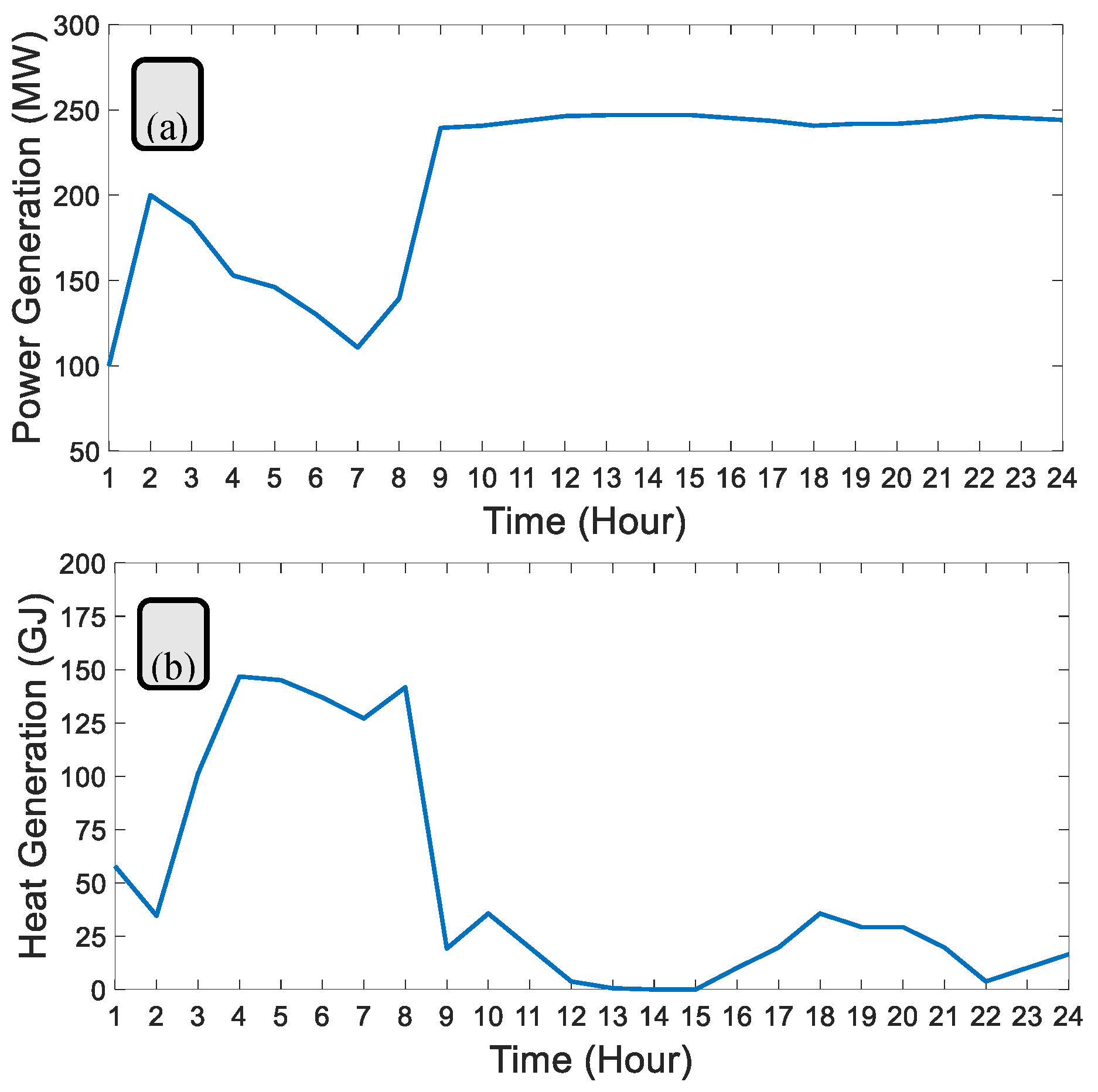
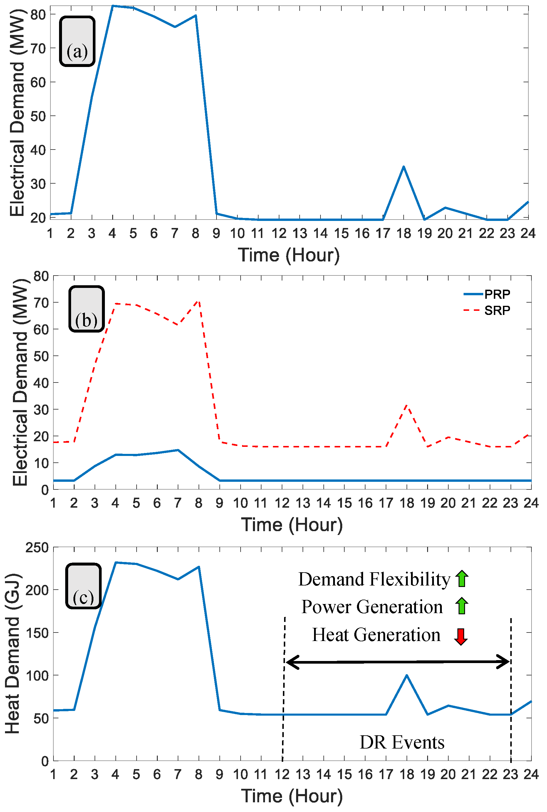
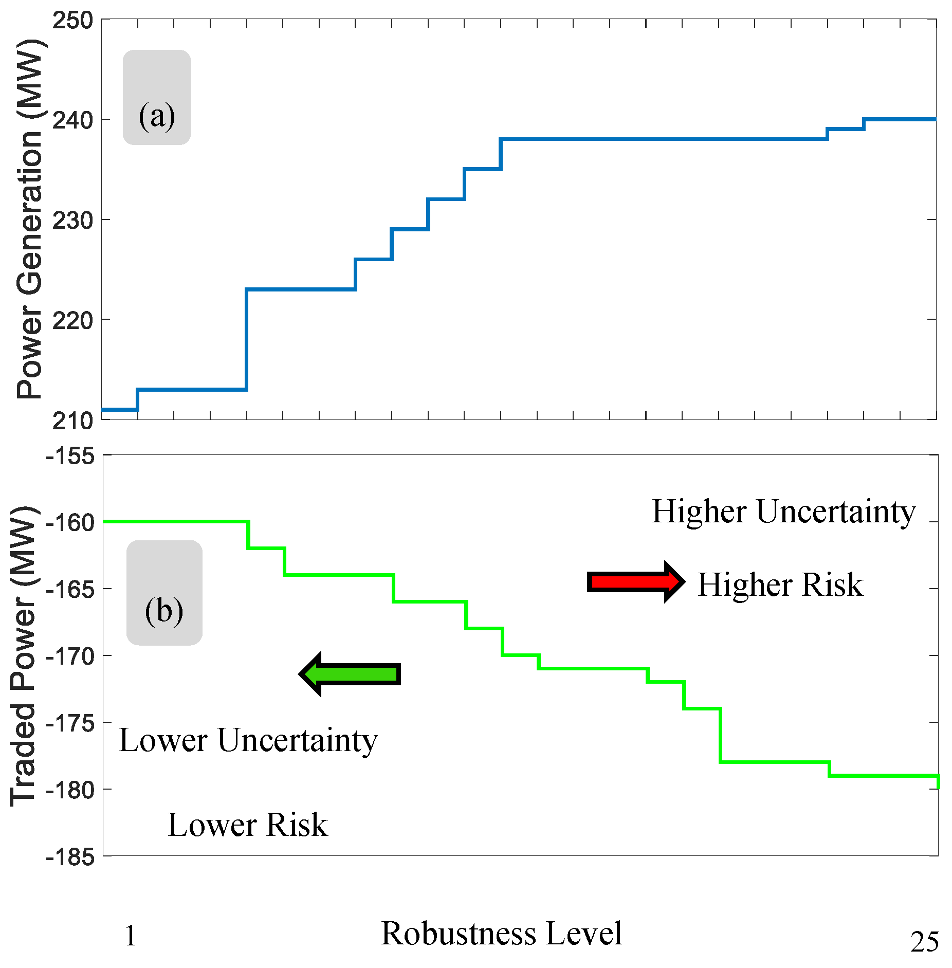
10.2. Results and Discussions

The main aim of the problem is to optimize the operation strategies of the test ORI, including procurement from the IEM, operation of refinery processes, and exploitation plans of CHP and boilers. Regarding the uncertain bound of electricity price, the procurement strategies are determined based on the worst-case realization of the electricity price.

First of all, Figure 9 describes the exploitation plan of CHP in terms of power and heat generations. Subfigure (a) shows the power generation of the CHP. Based on the graph, the CHP generates moderate electricity during off-peak hours, i.e., 1 to 8. In contrast, the electricity generation increases considerably from 9 to 24 when the day and night peak durations occur. Therefore, the CHP reaches the upper threshold of power generation in critical hours of the IEM, to provide power flexibility to the electricity market. Besides, subfigure (b) illustrates the heat generation of the CHP. As the graph reveals, the CHP produces a large amount of steam during hours 2 to 9, when the steam demand of the ORI is high (see the steam demand of the ORI in Figure 10). Adversely, the steam generation of the CHP decreases significantly during DR events, i.e., 9 to 24. There are two reasons to justify this fact. Firstly, the steam demand of the ORI is mainly supplied out of DR events in hours 2 to 9 (based on Figure 10). Besides, in the DR events, electrical power is the clear need for the IEM. Therefore, considering the FOR of the CHP in Figure 3, the CHP working point reaches the upper threshold of power generation, i.e., point A, which generates a low amount of heat.

Figure 10 illustrates the optimized operation of the ORI for 24 h. As subfigure (a) reveals, the largest amount of electricity consumption of the ORI is scheduled out of DR events. During the DR events, the ORI decreases the electricity consumption significantly to provide power flexibility to the upstream network. Subfigure (b) shows the electricity consumption of the PRP and SRP. Based on the graph, the two industrial sub-processes follow a similar pattern to maximize the demand-side flexibility of the ORI. Furthermore, subfigure (c) illustrates the total steam demand of the ORI. As can be seen, the steam demand of the ORI reaches the lowest point during DR events. Considering the FOR of the CHP in Figure 3, this enables the CHP to reach the upper threshold of electricity generation to overcome the power shortage in the IEM during the DR events. This is an interesting result that shows how the correlation between joint heat-electricity generation can be optimized to not only provide power flexibility to the electricity market, but also supply the joint electricity-heat demand of the industry.

Figure 11 describes the optimized operation of the industrial boiler. As the line graph reveals, the boiler generates a huge amount of steam out of DR events, i.e., hours 3 to 10. The reason is that the main part of the ORI operation is scheduled in this duration. To continue, the steam generation of the boiler decreases as the steam demand of the ORI reduces. It is worth mentioning that the boiler compensates for the lack of steam generation during DR events to help the CHP reach the upper threshold of power generation.

Figure 12 illustrates the hourly cumulative production of the ORI. Interpreting the figure, interesting results are obtained. First of all, the curve can be divided into two main areas representing DR events and out of DR events. The production rates for these two areas are shown with two symbolic ramps, m₁ and m₂. As the graph reveals, the value of m₁ is larger than m₂ (m₁ > m₂). This confirms that the industry schedules the industrial operation, mainly out of DR events. Approaching the DR duration, the ramp rate of production decreases moderately. In this way, hour 10 can be considered as a milestone, where the industry makes it ready to reduce the energy consumption 2 h before the DR event. The gap between the milestone and the beginning time of the DR event is caused due to technical constraints of the industry when the plant cannot change the energy consumption suddenly. Heat and electrical ramp rates of industrial sub-processes are the main constraints to determine the duration of the gap time. Finally, the cumulative production meets the daily ordered value of 44 kt.

Figure 13 illustrates the power traded in the IEM. The bar graph conveys the electricity sold to the wholesale electricity market. Based on the graph, the ORI prefers to use the self-generation facilities as the main electricity supply out of DR events when the electricity market price is relatively low. Therefore, the ORI consumes the power generation of the CHP for the internal processes. In contrast, during DR events, the ORI sells much more electrical power to the electricity market when the market price reaches the highest level in the day. As can be seen, the traded power reaches the highest point in hours 12–16 and 21–22 to provide flexibility to the power system in day and night peak hours. The sold power experiences a slight reduction between hours 16 and 21. This time duration is a gap time between day and night peaks of the IPG, which is followed by the ORI considering the ramp-up/-down of the CHP. Trading power in high price hours, the ORI increases the profit. Therefore, the ORI not only participate in the peak shaving of the upstream network, but also takes advantage of increased profit. As a result, both beneficiaries, including the ORI and IEM, take advantage of cost optimization and flexibility potential, respectively.

Figure 14 describes the total electrical demands of the ORI in response to the daily demand profile of the IPG. In the summer, the IPG experiences two peak durations during a day. The day peak normally occurs when the electrical demand of residential cooling systems increases significantly, i.e., hours 12–16. The night peak emanates from the increased lighting system of residential and commercial sectors. Therefore, the responsive plants should provide power flexibility in both peak durations. In Figure 14, the daily demand profile of the IPG is depicted in subfigure (b). Based on the graph, the industry can provide applicable flexibility to the IPG in both peak hours. In addition, the electricity consumption of the ORI increases moderately between the two peak slots, i.e., hours 17–19. Based on the line graph, as the ORI responds to the DR events, the peak demand of the plant is shifted out of DR events. In this way, the need for installing fast-run power generation facilities in the IPG is obviated.

Figure 15 illustrates the role of storage in providing power flexibility to the IPG. The graph is depicted in three states, considering 100, 50, and 25 percent of the original storage capacity. As the graph reveals, decreasing the storage capacity, the power demand of the industry moves to the DR events. Therefore, the capacity of the industry to provide power flexibility to the IPG decreases noticeably.

Figure 16 illustrates the robust decisions of the ORI. The robust values, including power generation of CHP and traded power in the wholesale market, corresponding to each robustness level are the average values of the decision variables for 24 h. Firstly, subfigure (a) shows the robust decisions of the electrical power generation of the CHP. Based on the graph, as the robustness level increases, the ORI prefers to generate more electrical energy through the self-generation facilities. In fact, by increasing the electricity price uncertainty, the industry decides to sell more energy to the electricity market. This is an interesting result that shows that risk-taker participants prefer to trade more energy in uncertain markets. Besides, subfigure (b) describes the robust decisions of the traded power in the electricity market. Following a similar pattern, as the robustness level increases, the risk-taker industry trades more energy in the uncertain market. Indeed, the risk-taker participants prefer to trade more energy in an uncertain electricity market. It is worth mentioning that a lower amount of robustness levels indicates lower uncertainty. A risk-averse participant prefers to work in this state. In contrast, a high amount of robustness level corresponds to higher uncertainty that is preferred by risk-taker market traders.

From the risk-bearing viewpoint, Figure 16 conveys two different aspects:

(1)

Risk-taker market participants

(2)

Risk-averse market participants

The risk-taker participants consider high levels of uncertainty in operational scheduling. Therefore, this type of participant prefers to participate in electricity market floors with high price uncertainty. In this study, the industry can supply the required energy from the self-generation facilities and the wholesale market. From the uncertainty viewpoint, the self-generation facilities have no uncertainty in the electricity price. In contrast, the wholesale market imposes a great deal of uncertainty in the electricity price. In such a situation, the risk-taker participants prefer to participate in the wholesale electricity market to make a profit in the uncertain electricity market. In fact, the risk-taker participants bear the burden of the market price uncertainty to make more profit. Adversely, risk-averse participants prefer not to purchase their required energy from the uncertain wholesale market. In this way, the risk-averse participants prefer to supply their energy from the self-generation facilities without price uncertainty.

Figure 17 illustrates the benefits of power trading in the wholesale electricity market. The benefits are described in terms of profit and flexibility. First of all, as the graph reveals, the ORI provides a relatively high income from selling energy to the wholesale market. In this way, an income of 378.7 × 10³ $ is provided by selling power to the wholesale market. Besides, based on the graph, most energy is injected to the IPG during hours 12–16 and 20–23, i.e., day and night peak hours. Therefore, the ORI is successful to provide power flexibility to the market during the daily peak hours. To sum up, the suggested approach not only provides power flexibility to the market, but also increases the income of the industry.

In industrial studies, the superiority of the suggested approaches should be investigated in comparison with the literature [34]. In this way, the key results are pointed out to show how the proposed approach outweighs the previous studies [35,36]. Therefore, the final results can be stated as follows:

(1)

Integration of joint heat-power flexibility to electricity markets with price uncertainty.

(2)

Cost-effective energy management for oil refinery industries, not only to provide demand-side flexibility to the electricity market, but also to increase the industries’ profit.

11. Conclusions

This paper proposed a novel structure to provide demand-side flexibility to the electricity market with price uncertainties. To achieve the aim, industrial sub-processes of a heavy oil refinery plant were modeled mathematically. The main feature of the problem was the integration of joint heat-power flexibility to the upstream network. To overcome the electricity price uncertainty, an iterative robust approach was suggested to determine the optimized exploitation plans of the industry under the worst-case realization of electricity prices. Moreover, to show the correlation between heat and power in providing demand-side flexibility, CHP and industrial boilers were simulated as self-generation facilities.

Simulation results showed that the CHP generated moderate values of electrical power and high values of heat out of DR events. In contrast, the CHP reached the highest level of power generation in DR events to provide flexibility to the power system. In this situation, the value of steam generation reduced significantly during DR events.

The ORI scheduled the main electricity consumption out of DR events. Therefore, the heat demand during DR events decreased considerably. This was the reason why the CHP generated less heat in DR duration. This stems from the fact that the power generation of CHP was injected into the outer network while the steam must be consumed in the internal processes.

Regarding the output production of the industry, the rate of production decreased considerably before the beginning of the DR events. In this way, a milestone can be detected in the production curve, followed by a gap time. This was a critical point for energy experts at the Department of Production Planning to respond to DR events on short or long notice. Ramp-up/-down rates of CHP and boilers played an important role in determining the value of gap time where the industrial sub-processes needed enough time to be turned down.

Finally, comparing the total electricity demand of the industry in responsive and non-responsive (traditional) states, it was shown that the plant can provide power flexibility to the upstream network; up to 72% of the nominal power. All in all, the results confirmed that the approach not only provides flexibility to the electricity market, but also increased the profit of the industry.

References

1. Golmohamadi, H.; Keypour, R.; Bak-Jensen, B.; Pillai, J.R.; Khooban, M.H. Robust Self-Scheduling of Operational Processes for Industrial Demand Response Aggregators. IEEE Trans. Ind. Electron. 2020, 67, 1387–1395. [Google Scholar] [CrossRef] [Green Version]
2. Golmohamadi, H.; Keypour, R.; Bak-Jensen, B.; Pillai, J.R. A multi-agent based optimization of residential and industrial demand response aggregators. Int. J. Electr. Power Energy Syst. 2019, 107, 472–485. [Google Scholar] [CrossRef]
3. James, D.G.; Gary, H.; James; Handwerk, H.; Mark; Kaiser, J. Petroleum Refining Technology and Economics; CRC Press: Boca Raton, FL, USA, 2007. [Google Scholar]
4. Branco, D.A.C.; Gomes, G.L.; Szklo, A.S. Challenges and technological opportunities for the oil refining industry: A Brazilian refinery case. Energy Policy 2010, 38, 3098–3105. [Google Scholar] [CrossRef]
5. Wu, N.; Chu, C.; Chu, F.; Zhou, M. Schedulability Analysis of Short-Term Scheduling for Crude Oil Operations in Refinery With Oil Residency Time and Charging-Tank-Switch-Overlap Constraints. IEEE Trans. Autom. Sci. Eng. 2011, 8, 190–204. [Google Scholar] [CrossRef]
6. Bayat, M.; Aminian, J.; Bazmi, M.; Shahhosseini, S.; Sharifi, K. CFD modeling of fouling in crude oil pre-heaters. Energy Convers. Manag. 2012, 64, 344–350. [Google Scholar] [CrossRef]
7. Johansson, D.; Franck, P.-Å.; Berntsson, T. CO2 capture in oil refineries: Assessment of the capture avoidance costs associated with different heat supply options in a future energy market. Energy Convers. Manag. 2013, 66, 127–142. [Google Scholar] [CrossRef]
8. Flores, L.I.R.; García, J.A.E. Modernization of National Oil Industry in Mexico: Upgrading With IEC61850. IEEE Access 2014, 2, 571–576. [Google Scholar] [CrossRef]
9. Zhou, L.; Liao, Z.; Wang, J.; Jiang, B.; Yang, Y.; Du, W. Energy configuration and operation optimization of refinery fuel gas networks. Appl. Energy 2015, 139, 365–375. [Google Scholar] [CrossRef]
10. Yang, Q.; Qian, Y.; Zhou, H.; Yang, S. Conceptual design and techno-economic evaluation of efficient oil shale refinery processes ingratiated with oil and gas products upgradation. Energy Convers. Manag. 2016, 126, 898–908. [Google Scholar] [CrossRef]
11. Eldean, M.A.S.; Soliman, A.M. A novel study of using oil refinery plants waste gases for thermal desalination and electric power generation: Energy, exergy & cost evaluations. Appl. Energy 2017, 195, 453–477. [Google Scholar] [CrossRef]
12. Khodabakhsh, A.; Arí, I.; Bakír, M.; Ercan, A.O. Multivariate Sensor Data Analysis for Oil Refineries and Multi-mode Identification of System Behavior in Real-time. IEEE Access 2018, 6, 64389–64405. [Google Scholar] [CrossRef]
13. Renzi, M.; Rudolf, P.; Štefan, D.; Nigro, A.; Rossi, M. Installation of an axial Pump-as-Turbine (PaT) in a wastewater sewer of an oil refinery: A case study. Appl. Energy 2019, 250, 665–676. [Google Scholar] [CrossRef]
14. Ashok, S.; Banerjee, R. Optimal operation of industrial cogeneration for load management. IEEE Trans. Power Syst. 2003, 18, 931–937. [Google Scholar] [CrossRef]
15. Gholian, A.; Mohsenian-Rad, H.; Hua, Y.; Qin, J. Optimal industrial load control in smart grid: A case study for oil refineries. In Proceedings of the 2013 IEEE Power Energy Society General Meeting, Vancouver, BC, Canada, 21–25 July 2013; pp. 1–5. [Google Scholar] [CrossRef]
16. Alarfaj, O.; Bhattacharya, K. Material Flow Based Power Demand Modeling of an Oil Refinery Process for Optimal Energy Management. IEEE Trans. Power Syst. 2019, 34, 2312–2321. [Google Scholar] [CrossRef]
17. Rivero, R.; Garcia, M.; Urquiza, J. Simulation, exergy analysis and application of diabatic distillation to a tertiary amyl methyl ether production unit of a crude oil refinery. Energy 2004, 29, 467–489. [Google Scholar] [CrossRef]
18. Kumar, A.; Gautami, G.; Khanam, S. Hydrogen distribution in the refinery using mathematical modeling. Energy 2010, 35, 3763–3772. [Google Scholar] [CrossRef]
19. Weijermars, R. Accelerating the three dimensions of E&P clockspeed—A novel strategy for optimizing utility in the Oil & Gas industry. Appl. Energy 2009, 86, 2222–2243. [Google Scholar] [CrossRef]
20. Gueddar, T.; Dua, V. Novel model reduction techniques for refinery-wide energy optimisation. Appl. Energy 2012, 89, 117–126. [Google Scholar] [CrossRef]
21. Coatalem, M.; Mazauric, V.; le Pape-Gardeux, C.; Maïzi, N. Optimizing industries’ power generation assets on the electricity markets. Appl. Energy 2017, 185, 1744–1756. [Google Scholar] [CrossRef]
22. Mete, E.; Turkay, M. Energy Network Optimization in an Oil Refinery. In 13 International Symposium on Process Systems Engineering (PSE 2018); Eden, M.R., Ierapetritou, M.G., Towler, G.E., Eds.; Elsevier: Amsterdam, The Netherlands, 2018; Volume 44, pp. 1897–1902. [Google Scholar]
23. The International Council of Clean Transportation. An Introduction to Petroleum Refining and the Production of Ultra Low Sulfur Gasoline and Diesel Fuel; MathPro: Bethesda, MD, USA, 2011. [Google Scholar]
24. Golmohamadi, H.; Keypour, R.; Mirzazade, P. Multi-objective co-optimization of power and heat in urban areas considering local air pollution. Eng. Sci. Technol. Int. J. 2020. [Google Scholar] [CrossRef]
25. Golmohamadi, H.; Keypour, R. Retail Energy Management in Electricity Markets: Structure, Challenges and Economic Aspects—A Review. Technol. Econ. Smart Grids Sustain. Energy 2017, 2, 20. [Google Scholar] [CrossRef] [Green Version]
26. Golmohamadi, H.; Keypour, R. A bi-level robust optimization model to determine retail electricity price in presence of a significant number of invisible solar sites. Sustain. Energy Grids Netw. 2018, 13, 93–111. [Google Scholar] [CrossRef]
27. Golmohamadi, H.; Keypour, R. Application of Robust Optimization Approach to Determine Optimal Retail Electricity Price in Presence of Intermittent and Conventional Distributed Generation Considering Demand Response. J. Control. Autom. Electr. Syst. 2017, 28, 664–678. [Google Scholar] [CrossRef]
28. Golmohamadi, H.; Keypour, R.; Hassanpour, A.; Davoudi, M. Optimization of green energy portfolio in retail market using stochastic programming. In Proceedings of the 2015 North American Power Symposium (NAPS), Charlotte, NC, USA, 4–6 October 2015; pp. 1–6. [Google Scholar] [CrossRef]
29. International Energy Agency, IEA. 2020. Available online: https://www.iea.org/ (accessed on 3 February 2020).
30. Iran Grid Management Company (IGMC). 2019. Available online: https://www.igmc.ir/Power-grid-status-report (accessed on 11 January 2019).
31. GAMS Software. Available online: https://www.gams.com/ (accessed on 2 April 2019).
32. CPLEX Solver. Available online: https://www.ibm.com/dk-en/analytics/cplex-optimizer (accessed on 11 July 2019).
33. CONOPT Solver. Available online: http://www.conopt.com/ (accessed on 11 July 2019).
34. Zhang, Z.; Ding, S.; Sun, Y. A support vector regression model hybridized with chaotic krill herd algorithm and empirical mode decomposition for regression task. Neurocomputing 2020, 410, 185–201. [Google Scholar] [CrossRef]
35. Zhang, Z.; Ding, S.; Jia, W. A hybrid optimization algorithm based on cuckoo search and differential evolution for solving constrained engineering problems. Eng. Appl. Artif. Intell. 2019, 85, 254–268. [Google Scholar] [CrossRef]
36. Li, M.-W.; Geng, J.; Hong, W.-C.; Zhang, L.-D. Periodogram estimation based on LSSVR-CCPSO compensation for forecasting ship motion. Nonlinear Dyn. 2019, 97, 2579–2594. [Google Scholar] [CrossRef]
Figure 1. Flow diagram of the literature on the oil refining industries (ORI), with the clear need for future research.
Energies 13 04874 g001
Figure 2. Industrial subprocesses of a modern ORI.
Energies 13 04874 g002
Figure 3. Heat-power feasible operation range (FOR) of the combined heat and power (CHP) [24].
Energies 13 04874 g003
Figure 4. Flow diagram of operation between two consecutive refinery processes.
Energies 13 04874 g004
Figure 5. Robustness region for the electricity price uncertainty.
Energies 13 04874 g005
Figure 6. Coordination between different entities to provide demand flexibility for external grids.
Energies 13 04874 g006
Figure 7. The flowchart of the proposed approach with input and output data.
Energies 13 04874 g007
Figure 8. Robust bound of wholesale market price.
Energies 13 04874 g008
Figure 9. Optimized operation of CHP (a) power generation and (b) heat generation.
Energies 13 04874 g009
Figure 10. Optimized operation of the ORI in terms of (a) Total electricity demand (b) Electricity demand of two sub-processes and (c) Total heat demand.
Energies 13 04874 g010
Figure 11. Optimized steam generation of the industrial boiler.
Energies 13 04874 g011
Figure 12. Cumulative production of the ORI for 24 h.
Energies 13 04874 g012
Figure 13. Traded power in the wholesale electricity market.
Energies 13 04874 g013
Figure 14. (a) Optimized electrical demand of the ORI in response to (b) demand profile of Iran Power Grid (IPG).
Energies 13 04874 g014
Figure 15. Role of storage in peak shaving.
Energies 13 04874 g015
Figure 16. Robust decisions of the ORI in the uncertain electricity market (a) Power generation; (b) Traded power.
Energies 13 04874 g016
Figure 17. Benefits of selling electricity to the market in terms of income and power flexibility.
Energies 13 04874 g017