Recovery Mechanisms for Cyclic (Huff-n-Puff) Gas Injection in Unconventional Reservoirs: A Quantitative Evaluation Using Numerical Simulation

Abstract

Unconventional reservoirs produce large volumes of oil; however, recovery factors are low. While enhanced oil recovery (EOR) with cyclic gas injection can increase recovery factors in unconventional reservoirs, the mechanisms responsible for additional recovery are not well understood. We examined cyclic gas injection recovery mechanisms in unconventional reservoirs including oil swelling, viscosity reduction, vaporization, and pressure support using a numerical flow model as functions of reservoir fluid gas–oil ratio (GOR), and we conducted a sensitivity analysis of the mechanisms to reservoir properties and injection conditions. All mechanisms studied contributed to the additional recovery, but their significance varied with GOR. Pressure support provides a small response for all fluid types. Vaporization plays a role for all fluids but is most important for gas condensate reservoirs. Oil swelling impacts low-GOR oils but diminishes for higher-GOR oil. Viscosity reduction plays a minor role for low-GOR cases. As matrix permeability and fracture surface area increase, the importance of gas injection decreases because of the increased primary oil production. Changes to gas injection conditions that increase injection maturity (longer injection times, higher injection rates, and smaller fracture areas) result in more free gas and, for these cases, vaporization becomes important. Recovery mechanisms for cyclic gas injection are now better understood and can be adapted to varying conditions within unconventional plays, resulting in better EOR designs and improved recovery.

1. Introduction

Unconventional reservoirs such as the Eagle Ford, Bakken, and others have had tremendous success over the last decade. Production from these low-permeability, liquid-rich reservoirs has increased to over 8 million stock tank barrels per day (STB/day) in the US, which accounts for almost 65% of US oil production [1] and, in North America, these types of reservoirs have cumulatively produced over 10 billion barrels of oil. This success has been due to improvements in two important areas of the petroleum industry: extended-reach horizontal wells and multi-stage hydraulic fracturing. Possibly even more important than the high rates are the volumes of in-place oil for these unconventional reservoirs. In each formation, there are hundreds of billions of barrels of oil in place [2,3,4], which exceeds even the largest conventional reservoirs. These unconventional reservoirs served as the source rocks for many conventional reservoirs, and while much oil migrated out to fill higher-permeability reservoirs, even more has remained at the source.

However, there are still major issues to be addressed. The wells may start producing at very high rates, but the rates drop off quickly, and the wells have low recovery factors, generally less than 10% [5,6]. Even as longer horizontal wells and larger hydraulic fractures are implemented, the initial rates tend to get higher, but the general behavior remains the same—rapid decline and low overall recovery. Therefore, the need to develop methods to improve overall recovery is evident. Some increases from infill drilling and improvements in hydraulic fracturing have the potential to increase the recovery factors to some extent, but they are expected to continue to be much less than 20%. To achieve recovery factors of 20% and higher, some form of fluid injection is likely needed.

The value of enhanced oil recovery (EOR) for unconventional reservoirs like the Bakken and Eagle Ford was noted early in the production of these reservoirs [7,8], and there has been significant research over the last decade on this topic (summaries in Alfarge et al. [9] and Kanfar et al. [10]). Much of this early work was done in the laboratory (e.g., Jin et al. [11] and Tovar et al. [12]) or with numerical models (e.g., Li et al. [13] and Gala and Sharma [14]), where they looked at questions of overall recovery, the type of gas, soak time, vaporization, and utilization.

There have been a few field trials, but most data from them are held within the companies. The limited public data from these field trials were published for the Bakken [15] and the Eagle Ford [16], but many of the data were not available, such as bottom hole flowing pressures, injection rates/pressures, and producing gas–oil ratios. Therefore, it was difficult to validate the results from the laboratory experiments or the numerical models. Then, in 2013, a company started having success by injecting natural gas in the Eagle Ford in a cyclic manner where the injection wells and producing wells were the same, often called huff-n-puff gas injection. In May 2016, the company reported their results [17], which showed incremental recovery for the process to be between 30% and 70%.

Since that time, other companies have tried this process and found similar increases in oil recovery, but the reasons for the additional recovery have not been extensively reported. Understanding how fluid injection can help increase oil recovery from unconventional reservoirs will require a multi-pronged approach to fully comprehend the issues and develop solutions that work. This paper focuses on the recovery mechanisms for huff-n-puff natural gas injection projects to determine why additional oil is recovered.

Recovery mechanisms are important for understanding what is happening in the reservoir and for improving the overall recovery and efficiency. If the process is better understood, procedures can be developed to maximize the recovery efficiency; thus, more oil can be produced with less gas injected. Without understanding the recovery mechanisms, improving the process becomes an expensive trial-and-error endeavor.

There have been numerous recovery mechanisms proposed for gas injection into liquid-rich unconventional reservoirs. Nine are shown below, which should be considered a thorough but not exhaustive list.

• Vaporization;
• Viscosity reduction;
• Secondary solution gas drive;
• Interfacial tension reduction;
• Wettability changes;
• Oil swelling (expansion);
• Pressure support;
• Rock/fluid interactions;
• Injection-induced fracturing.

The first five mechanisms (vaporization, swelling, secondary solution gas drive, viscosity reduction, and pressure support) are the most often cited and appear to be the most significant from a literature review. This work focuses on these, but it does not mean that the other mechanisms are not important.

While there has been significant work with enhanced oil recovery (EOR) in unconventional reservoirs over the last decade, there has been little focus on the recovery mechanisms. Tovar et al. [18] used laboratory data to discuss the importance of vaporization and declared that it is the main recovery mechanism for gas injection EOR in organic rich shales. Hamdi et al. [19] discussed the complex function of mass transfer and extraction processes related to a number of different potential mechanisms. Hoffman and Rutledge [20] compared the role of diffusion and advection for the oil-swelling mechanism using analytical models. While these are good papers to start discussing mechanisms, they either focus on a single mechanism or have only a qualitative comparison of different mechanisms. A fully systematic and quantitative evaluation of different mechanisms is needed, which this paper intends to address.

This effort is inspired by and builds upon work done trying to understand the importance of various recovery mechanisms in thermal recovery/steam injection methods by Wu [21]. Burger et al. [22] published a chart showing how the relative significance of the mechanisms for thermal recovery changed as a function of the American Petroleum Institute (API) gravity of the oil (Figure 1).

Heavy (low API) oils are influenced by viscosity reduction, while thermal expansion and vaporization are more significant for lighter oils. While this is a qualitative view of recovery as a function of the oil density, a more quantitative evaluation was conducted for a medium-weight oil (22 API) as a function of pore volumes of steam injected [23]. For this oil, all mechanisms contribute significantly; this work also showed that the relative importance of the mechanisms changes slightly as a function of pore volumes injected or time (Figure 2)

While huff-n-puff gas injection into unconventional reservoirs is different to thermal recovery, a similar approach can be used to evaluate the mechanisms, including determining the recovery as a function of fluid properties. The in-situ fluid properties can change dramatically across an unconventional basin. The Eagle Ford is a good example, where, from northwest to southeast, the fluid goes from a low gas–oil ratio (GOR) (<500 standard cubic feet per stock tank barrel (scf/STB)) black oil to a dry gas, as shown in Figure 3.

Unlike conventional reservoirs, deeper zones have more gas due to the higher temperatures needed for gas generation. This is called an inverted petroleum system. Huff-n-puff gas injection has occurred from the black low-GOR oils to high-GOR volatile oils and the gas condensate regions of the Eagle Ford. Therefore, we evaluated the recovery mechanisms as a function of GORs ranging from 500 scf/STB to 20,000 scf/STB.

In addition to the study of recovery mechanisms with respect to GOR, the sensitivity of the recovery mechanisms to reservoir properties and huff-n-puff operational parameters is also investigated. We focus on the case with a GOR of 1200 scf/STB and evaluate a wide range of reservoir and operational parameters to understand how the recovery mechanisms are impacted.

2. Reservoir Model

For this study, reservoir models were constructed to simulate the production from a liquid-rich unconventional reservoir undergoing a huff-n-puff type gas injection process. The models were used to assess (1) the contributions from various production mechanisms to the incremental production resulting from the gas injection, and (2) the sensitivity of various reservoir and gas injection parameters to the production mechanisms.

Two reservoir models were used for the study: a larger-scale single-well sector model and a smaller-scale quarter-fracture model based on the single well model. The single-well model was used for the initial history match and investigation of the influence of the GOR on the EOR mechanisms. This model was also used to study the effects of hydraulic fracture density on the EOR mechanisms. The smaller quarter-fracture model was used to investigate the effects of additional reservoir and EOR injection/production parameters on the EOR mechanisms. The development of the models is discussed below.

2.1. Single-Well Model

The single-well model simulated a hydraulically fractured horizontal well in a low-permeability liquid-rich unconventional reservoir. It represents a typical well such as those currently being drilled in the Bakken, Eagle Ford, Permian, or other source rock basins. Because most of the gas injection projects in unconventional reservoirs occurred in the Eagle Ford, typical properties from the Eagle Ford were used. Furthermore, the model was validated by history-matching it to an Eagle Ford cyclic gas injection field pilot dataset.

The model is representative of a single well in an eight-well-per-section pattern. It is 10,550 ft (~2 miles) long and 650 feet wide. The model is 72 ft thick, which is a typical value for the Lower Eagle Ford. The grid blocks are 50 ft × 50 ft × 8 ft; thus, there are 13 in the x-direction, 211 in the Y-direction, and nine in the z-direction. There is a single 9550 ft long horizontal well through the middle of the model (z = 5), leaving 500 feet on each end (Figure 4).

There are 40 hydraulic fractures along the wellbore modeled as planar, parallel, equidistant features 250 feet apart (Figure 4).While hydraulic fractures are often considered to have complexity with fractures occurring in multiple directions, for gas injection, the fracture surface area in contact with the matrix is one of the most important attributes for recovering additional hydrocarbons. In this model, simple planar fractures are used that have the same surface area as the more complex ones; thus, they can be considered as reasonable approximations [20]. For this model, the total surface area of the fractures is 3.7 million ft². In a recent study, a core was taken from a well near a previous well that was hydraulically fractured [25]. In that study, they estimated the amount of fracture surface area in a modern multistage fracture stimulation, and it is comparable to the value used in this study. The permeability of the hydraulic fractures was determined through the history-matching process.

The hydraulic fractures are modeled as discrete fractures that interact with the matrix and wells through the non-neighbor connections using a dual permeability formulation. The matrix properties were assumed to be homogeneous throughout the model and set to 8% porosity and 100 nanodarcys (nd) [26]. The initial water saturation was set at 37.5% which is the range of water saturations observed for the Eagle Ford [26]. Since, in many places, little water is produced from the Eagle Ford, we assumed that the initial water was also the irreducible water saturation. This allowed the water pore volume to be removed from the model, improving the simulation performance and having negligible effects on the results.

The pore volume of the fractures was controlled by setting the porosity values for the fracture gridblocks (${\varnothing }_{gb}$) to very small values using Equation (1).

$$w_{gb}{\varnothing }_{gb}=w_f{\varnothing }_f,$$

(1)

where w_gb is the width of the gridblocks, which in this case was 50 ft, and w_f is the actual width of the fracture, which was assumed to be 1/8 of inch in this case. A 24% fracture porosity (${\varnothing }_f$) was assumed. Therefore, the porosity, ${\varnothing }_{gb}$, used in the fracture gridblocks was 0.00005 (0.005%) resulting in a 50 ft gridblock representing a 1/8-inch fracture.

Pressure-dependent permeability is often used to simulate changes in permeability resulting from pressure depletion in unconventional reservoirs [7,27,28,29]. This accounts for the micro and meso fractures (less than 50 ft) in the reservoir that close and reduce permeability as pressure is reduced. Therefore, a pressure-dependent permeability function was included in the model for the matrix blocks (Figure 5) and used as a history-matching parameter. The fracture gridblocks did not have pressure-dependent permeability since it is so much greater than the matrix permeability that it had insignificant impacts on the overall results. The curve shown in Figure 5 is the final history-matched pressure-dependent permeability function. As gas is injected back into the reservoir, it will likely reopen these weak planes and increase permeability; thus, this pressure-dependent permeability is also reversible.

Figure 6 shows the relative permeability for both the matrix and the fractures. Straight-line relative permeability is used for the fractures, whereas typical Corey-type curves are used for the matrix. The matrix gas relative permeability in Figure 6a includes changes needed to history-match the gas injection process. The capillary pressure was set to zero for this gas–oil system.

The initial reservoir pressure was 5500 pounds per square inch (psi). The producing bottom hole pressure (BHP) was constrained to 500 psi, as we assumed that the well is operating efficiently. During the injection cycles, the well was constrained to a gas injection rate of 1000 Mscf/day. The BHP pressure increased during injection, but never exceeded 6500 psi. For the base model, which is a 1200 scf/STB GOR fluid, the bubble point pressure (Pb) was 3200 psi.

2.2. Fluid Model

For this research, the fluid model is one the most important aspects, and a significant amount of effort was spent on the fluid description. Initially, we planned to create a compositional fluid model, but that type of model is not able to evaluate the mechanisms of viscosity reduction or oil swelling (expansion) on recovery. A properly constructed black-oil model, however, could evaluate these mechanisms along with vaporization and pressure support. Therefore, a black-oil formulation with dissolved gas in the liquid phase and vaporized oil in the gas phase was used.

Whitson and Sunjerga [30] published the mole fraction compositions for plausible Eagle Ford in situ hydrocarbons for a wide range of GORs from which we selected three different base fluid types for our fluid models: a 1200 scf/STB GOR black oil, a 4000 scf/STB volatile oil, and a 10,000 scf/STB gas condensate. Compositions for the three different reservoir fluids were imported into a reservoir fluid property simulator, PVTi [31], along with the data from differential liberation (DL), constant composition expansion (CCE), and constant volume depletion (CVD) experiments that were obtained from Whitson and Sunjerga [30]. Each fluid was then matched to its GOR and bubble-point pressure (Pb) or dew-point pressure (Pd), and the black-oil simulation properties were exported for live oil and wet gas using the Whitson and Torp method [32]. To get a larger range of fluid types, the initial GOR was increased and/or decreased for each base fluid, and additional cases were run for each of those.

Table 1. Initial gas–oil ratios (GORs) and bubble-point pressures (Pb) or dew-point pressures (Pd) for the 12 different fluid models; 1200 standard cubic feet per stock tank barrel (scf/STB) is the base case. Pb is for black oil and volatile oil fluids, whereas Pd is for gas condensate reservoirs.

	Black Oil					Volatile Oil			Gas Condensate
GOR (scf/STB)	500	1000	1200	1400	1800	2400	3100	4000	6200	10,000	14,500	20,000
Pb/Pd (psi)	1900	2900	3200	3550	4100	4650	5100	5500	4450	4000	3300	2650

shows the GOR and respective bubble-point and dew-point pressures for all 12 cases.

2.3. History-Matching Single-Well Model

The single-well model was history-matched to data from a gas injection huff-n-puff pilot well in the Eagle Ford. This provided confidence that the properties used in the model were reasonable. Parameters changed in the matching process included matrix permeability, hydraulic fracture permeability, pressure dependent permeability, and relative permeability. The final history-match is shown in (Figure 7) and it is very close to the field data

The early peak production from the model was a little high. Early in the life of the well, when it is flowing under natural energy, the BHP may be higher than 500 psi, which could be why the model over-predicted the oil rates at early times. Since the wells were on for a few months before peak production (when the model was started), the cumulative recovery is within 5% error. Most importantly, the oil production during the gas injection phase matched very closely.

Table 2. Reservoir model properties. BHP, bottom hole pressure.

Property	Value	Property	Value
Matrix Permeability	100 nd	Initial Pressure	5500 psi
Matrix Porosity	8%	Model x-Dimension	650 ft
Number fractures	40	Model y-Dimension	10,550 ft
Fracture Half-length, xf	325 ft	Model Thickness (z)	72 ft
Fracture Permeability	5 md	Well Length	9550 ft
Fracture Spacing	250 ft	Well Producing BHP	500 psi
Water Saturation, Sw	37.5%	Injection Rate	1 MMcf/d

lists the final properties used, which are the same as those mentioned in the previous subsection. These values were used for all the models that evaluated the recovery mechanisms.

2.4. Quarter-Fracture Model

The single-well model was reconstructed into a quarter-fracture model to represent one side of a half-fracture. This allowed for smaller gridblocks and enabled higher-resolution simulations that were required for much of the sensitivity analysis. A fracture half-length of 325 ft was used from the single-well model; therefore, the quarter-fracture model length was 325 ft. The distance between two fractures in the single-well model was 250 feet; thus, the width of the quarter-fracture model was half of that or 125 feet. The gridblocks parallel to the fracture were 1 ft wide; hence, there were 125 gridblocks. Figure 8 shows the new higher-resolution quarter-fracture model. All the other parameters in the small model were the same as the larger model.

The new model was run on primary production and with the same gas injection scenarios as the single-well model except for the 1/160 the injection rate—to mimic the smaller scale. The production from the small model was multiplied by 160 to get a rate that could be compared to the single-well model. Figure 9 shows the production from the gas injection case for both models and the measured data from the field trial that were used for history-matching the single-well model. The small model produced slightly less oil than the large model, especially early on, but the small model continued to match the field data well, even with no other changes to the model.

As an additional check on the model, the saturation and pressure changes in the near-fracture area were examined for the injection and production periods (Figure 10). Prior to injection, gas had come out of solution and acted as a primary solution gas drive. Once the gas saturation exceeded its critical value, it started flowing in the reservoir such that the producing GOR started to increase (Figure 10A). After gas injection started, the pressure started to increase, and the gas saturation decreased as gas was forced back into solution. Once the pressure in the matrix was above the bubble-point pressure, then all the gas was back into the oil phase (Figure 10B). When the well was put back on production, the pressure dropped below the bubble-point pressure again, and a secondary solution gas drive mechanism was initiated (Figure 10C). As the next cycle of injection began, the pressure was raised, and gas dissolved back into the oil. The process was repeated over the cycles of production and injection.

After many cycles, however, the bubble point of the in-situ reservoir fluids increased because the mix of the gas and oil changed with each cycle. This is a common behavior described as the variable bubble-point pressure [33]. For late cycles, some free gas remained in the reservoir during injection (Figure 10D); this is partially because the pressure was not as high as early injection cycles and partially due to the variable bubble-point pressure.

3. Methodology to Isolate Unique Recovery Mechanisms

After the model was validated through history-matching, it was used to assess the different recovery mechanisms. This novel approach uses the flow simulator in a unique manner to model phenomena that cannot be evaluated in real reservoirs. In the real reservoir, all of the mechanisms are happening at the same time and it is impossible to separate the contribution of each one; however, since the physical behaviors are simply equations in the simulator, they can be turned on and off in the model to isolate the contribution of individual mechanisms. The paragraphs below describe in more detail how the production for the various recovery mechanisms was isolated.

The amount of oil recovered due to swelling or expansion is equal to the change in the oil formation volume factor. Therefore, if the oil formation volume factor term (Bo) is set to a constant value corresponding to its average initial value for all pressures and solution GORs, then the change in Bo is always zero, and the contribution from oil expansion is essentially turned off.

To turn off the vaporization mechanism, the vaporized oil–gas ratio term, Rv, was set to zero for all pressures resulting in no liquids being vaporized into the gas phase and, therefore, there was no contribution due to vaporization. When this happens, the recovery is only a function of the other mechanisms. Similarly, the oil viscosity term (μo) can be set to a constant value that corresponds to average initial viscosity. When gas dissolves into the oil, the viscosity in the model stays the same; thus, there is no additional oil production from reducing viscosity.

For this evaluation, the production was simulated for a total of just over 5 years. Gas injection occurred for the last 3 years and 2 months, mimicking the field test shown in Figure 9. The process below outlines how the contributions from the different recovery mechanisms were determined for varying fluid GORs. This process was also used for the sensitivity analysis.

A base case or primary model without gas injection was constructed for a given set of fluid properties with a unique initial GOR and run on primary production for just over 5 years. In addition to knowing the initial GOR, the initial values of Bo and μo were also known. The cumulative recovery at the end of the model run was recorded, and a restart file was output when gas injection would have started, in this case, 1 November 2014.

Next, a gas injection huff-n-puff case that included all recovery mechanisms and mimicked the injection and producing times from the field trials shown in Figure 9 was run. Since the first 2 years of production were the same as for the base case, the restart file was used to run the model starting in November 2014. In this case, all the mechanisms contributed to the recovery. The cumulative recovery at the end of the model run was also recorded. The difference in the production from the gas injection case and the base case represents the total increase in production due to the gas injection.

To determine the contribution from pressure support, all the gas injection recovery mechanisms except pressure support were shut off. This was done by setting Bo and μo to the respective constant initial values and setting Rv to zero. The model was again restarted in November 2014 so that these changes did not impact the primary recovery. The cumulative recovery at the end of the model run (31 December 2018) was recorded. The difference between this cumulative recovery and the cumulative recovery from the primary model is the contribution due to pressure support.

The contribution from the expansion mechanism was determined by setting Bo to the original values and setting μo to a constant value and Rv to zero and running the model beginning in November 2014 using the restart file. The difference between this cumulative recovery and the cumulative recovery from the base case run is the contribution due to oil expansion. This process was repeated for the vaporization mechanism by setting Rv to the original values and setting Bo and μo to constant values. For the viscosity reduction mechanism, μo was set to the original values and Bo to a constant value and Rv to zero.

To further validate the method, the contributions from the four different mechanisms were summed, which should be approximately equal to the difference between the full gas injection model and the primary model. The relative importance of each mechanism can be determined by dividing each individual contribution by the total additional recovery due to gas injection.

The results can also be checked by making three more runs. In these runs, all the mechanisms are turned on except the one being investigated. The contribution of that mechanism is determined by calculating the difference in cumulative recovery between that run and the run where all the mechanisms are turned on, i.e., full gas injection case. Once all the contributions are calculated, the relative importance of each one can be determined as before.

Due to the numerical nature of the solutions, the results should not be exactly the same, but they should be close to each other, within 10% to 20%. If they are not, the models may have to be interrogated more closely for potential issues.

Once the results for this set of properties or injection parameters are satisfactory, a new fluid model is created with a different GOR and the above steps are repeated to find the relative importance of the different mechanisms for this new model.

In these simulations, it is not possible to distinguish between the additional oil produced due to liquid expansion versus the oil due to secondary solution gas drive. Both phenomena are related to the oil formation volume factor and cannot be individually turned on or off. Therefore, when evaluating the different recovery mechanisms, additional oil due to both liquid expansion and secondary solution gas drive are reported together.

Example

An example of the process is shown below for a 1200 scf/STB GOR oil. It is based upon the initial gas production from the field pilot test shown in Figure 9. This is also the model that was used to history-match the field data. Figure 11 shows the results from running (1) the primary production case, (2) the gas injection case, and (3) the injection case with the mechanisms turned off.

The difference between the primary production case (1) and the injection case with the mechanisms turned off (3) is the contribution due to pressure support. Figure 12a shows the incremental production due to oil swelling/solution gas drive (4), and Figure 12b shows the incremental production from vaporization (5). A similar plot could also be created for viscosity reduction.

Additionally, three new runs were completed. This time, instead of comparing each run to the “no mechanisms” case, they were compared to the “gas injection” case. Figure 13 shows how these runs were used to determine the contribution of different mechanisms. Adding up these differences is another way of determining the relative contribution of each mechanism and verifying the previous results.

The cumulative production for each case and the absolute and relative contributions for each of the mechanisms are shown in

Table 3. Results from simulation runs of 1200 scf/STB oil used to determine the relative contribution of different mechanisms.

Method 1				Method 2
	Cumulative Recovery (STB)	Relative Contribution (STB)	Fraction of Contribution\(%)		Cumulative Recovery (STB)	Relative Contribution (STB)	Fraction of Contribution (%)
Primary	125,700	--	--	Primary	125,700	--	--
No Mechanisms	138,000	12,300	14.5	Pressure Support	--	7600	9.0
Only Swelling	198,900	60,900	72.0	No Swelling	148,600	61,700	72.9
Only Vaporization	143,300	5300	6.3	No Vaporization	202,200	8100	9.6
Only Viscosity Reduction	144,100	6100	7.2	No Viscosity Reduction	203,100	7200	8.5
Gas Injection	210,300	84,600	100.0	Gas Injection	210,300	84,600	100.0

. The left side of the table (Method 1) shows the results when the mechanisms are turned on one-by-one and compared to the "no mechanisms case. To determine the pressure support contribution for these runs, the no mechanisms case was compared to the primary case. The right side of the table shows the additional comparison (Method 2) where one mechanism is turned off, and the contribution was determined by comparing each case to the full gas injection case. To determine the pressure support for this workflow, the primary cumulative recovery was subtracted from the gas injection, and then the relative contributions of the three other mechanisms were also subtracted from this number.

Both methods gave similar but not exactly the same results, which is expected with a numerical solution. The general trends, however, do appear to be the same. For this low-GOR oil, the oil-swelling mechanism appears to be the major source for the incremental oil production and the other three mechanisms make less meaningful contributions. Method 1 was used for the results presented in the next section.

4. Results

Results from both the study on the impact of reservoir fluid properties and the sensitivity analysis of the reservoir properties and gas injection parameters are presented in this section.

4.1. Reservoir Fluid Properties (GOR)

The process described in the previous section was completed for 12 different hydrocarbon systems ranging from 500 scf/STB to 20,000 scf/STB. Each evaluation was carried out as explained for the 1200 scf/STB oil. Figure 14 shows the total liquid recovery from primary production and for huff-n-puff gas injection for the different GORs. The cases are split into black oil, volatile oil, and gas condensate on the basis of the GOR. The incremental gas injection recovery is equal to the difference between bars in Figure 14.

Table 4. Percentage that each mechanism contributes to the recovery due to gas injection.

GOR	Pressure Support	Oil Swelling	Vaporization	Viscosity Reduction
500	21.9	65.8	2.5	9.8
1000	14.5	74.8	4.4	6.2
1200	14.5	72.0	6.3	7.2
1400	13.2	74.1	9.7	2.9
1800	6.3	71.6	20.9	1.1
2400	9.4	56.0	34.6	0.0
3100	4.5	55.4	40.2	0.0
4000	5.3	43.2	51.6	0.0
6200	8.5	10.6	80.9	0.0
10,000	7.1	7.1	85.7	0.0
14,500	6.7	6.7	86.7	0.0
20,000	6.3	6.3	87.5	0.0

shows the percentage that each mechanism contributes to the recovery from gas injection, and Figure 15A shows the same data in graphical form.

Oil swelling/secondary solution gas drive was most important for low-GOR oil and dropped off as GOR increases. The opposite was true for vaporization; its importance increased as GOR increases. This makes sense, but the results may be more extreme than expected. Since these are light oils, viscosity reduction played only a minor role for low GOR oils but overall did not contribute significantly for any case. Above a GOR of 1800 scf/STB, the pressure support contribution behaved somewhat erratically. For the 3100 scf/STB GOR case, the pressure support contribution was less than 5%; then, it bounced around between 5% and 9%. This may be due to the way the pressure support contribution was calculated. At lower GORs, it contributed 10% to 20%.

From Figure 15A, it is easy to see the importance of oil swelling for low-GOR hydrocarbons and vaporization for high-GOR ones. Figure 15B has the same ratios for the mechanisms, but the y-axis is the incremental oil production for gas injection over primary (the difference between bars in Figure 14.). In the highest-GOR cases, there was less liquid hydrocarbon to recover for both primary and EOR situations; thus, the incremental recovery for reservoirs with these fluid types was less.

Figure 16 again has the same ratios as Figure 16 but now the y-axis is the incremental recovery due to gas injection divided by the primary recovery. This gives the incremental percentage of recovery due to huff-n-puff gas injection. Depending on the GOR, the additional recovery was between 35% and 45%, which is reasonable when compared to field case studies with 3 years of injection. In Figure 16, the relative contribution is also broken down by the four different recovery mechanisms.

While Figure 15 and Figure 16 show a quantitative display of the results, Figure 17 represents a more qualitative view that summarizes the impacts of the mechanisms. The y-axis (efficiency) represents the EOR recovery divided by the primary recovery. This figure is similar to Figure 1 for thermal recovery.

4.2. Sensitivity Analysis

The sensitivity analysis was completed using the base case model with a 1200 scf/STB GOR fluid. Several model parameters could have an impact on the recovery and how much each mechanism contributed. The following is a partial list of the parameters that may influence the recovery:

• Permeability;
• Porosity;
• Initial pressure;
• Relative permeability;
• Critical gas saturation;
• Diffusion;
• Fracture surface area;
• Injection rate;
• Injection pressure;
• Cycle time;
• Total injection time;
• Bottom hole pressure;
• Injection gas composition;
• Wellbore length.

Some of the parameters were not included in the final analysis because they could not be implemented in the software (e.g., diffusion) and other parameters had similar behavior to each other (e.g., injection rate and injection pressure), but six different parameters were tested and because some parameters required two different changes (e.g., matrix permeability); thus, there were 9 unique models.

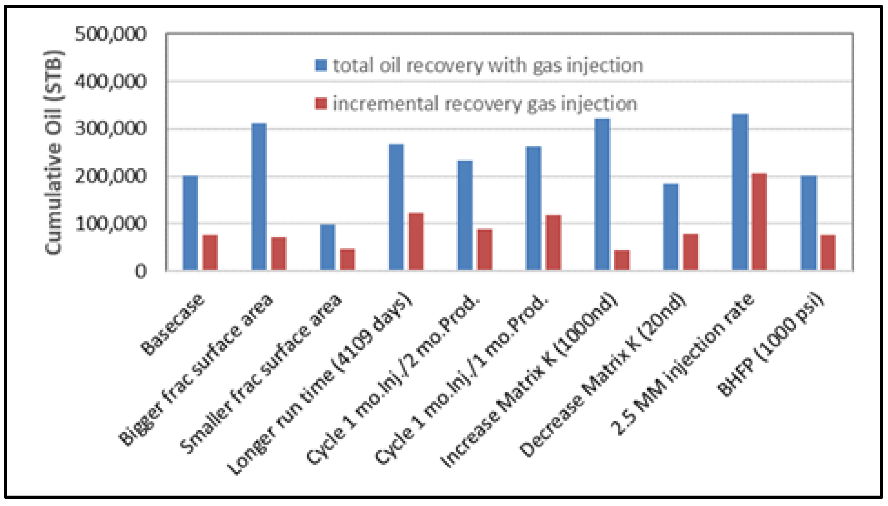
To begin with, all the models were run on primary production. Next, the models were run with gas injection with all the mechanisms turned on. Figure 18 shows the recovery for the base case and the nine other models. The taller (blue) columns represent the total oil recovered at the end of the gas injection, and the shorter (red) columns are for the incremental recovery. The difference between the two bars is the amount of oil that would have been produced on primary for that case.

Increasing the injection rate had the largest impact on overall recovery, which shows why getting gas into the reservoir is so important for these types of processes. Cases with more fractures and higher matrix permeability had increased overall production, but their incremental recoveries were not as great because they produced a lot of oil during the primary production stage of development. The case that ran the longest also had a big incremental increase, and the case with the smaller fracture area seems to be helped the most by gas injection, probably because there was the most amount of oil remaining. The sections below look at how the recovery mechanisms are affected by the various parameters.

4.2.1. Reservoir Rock Properties

The base case model had a matrix permeability of 100 nd. To evaluate the influence of matrix permeability, two additional models were created—one with a permeability of 1000 nd and one with a permeability of 20 nd. These are within the expected permeability range for unconventional oil reservoirs. Figure 19A shows the cumulative production for both the primary and gas injection cases.

For the higher-permeability case, from the time gas injection started until the end of the run, there was a lot of additional oil produced; however, during this time, the primary production also continued to increase and, thus, the relative contribution was not as much. For the two lower-permeability cases, the primary production leveled off; thus, the gas injection made a more significant contribution. If the high-permeability cases were run longer, the gas injection would have even more impact.

Figure 19B shows the relative influence of the different mechanisms. The two lower-permeability cases were about the same, but the higher-permeability case was influenced more by vaporization and oil swelling/solution gas drive and less by pressure support and viscosity reduction.

4.2.2. Fracture Surface Area

The area available for gas to interact with the oil in the matrix plays a significant role in the gas huff-n-puff process; therefore, different cases were built to evaluate the impact of the fracture surface area. The base case model had 40 hydraulic fractures with a total surface area of 3.7 million ft² (40 × 650 ft length × 72 ft height × 2 sides). Two additional cases were compared where the fracture area was doubled and halved. This was done simply by adding fractures closer to each other (an 80-fracture model) and removing fractures (a 20-fracture model).

Figure 20 shows the cumulative oil recovery forecasts for both primary and gas injection cases. The larger-surface-area case produced more on primary and more during EOR as there was more volume being accessed by the fractures. It appeared to increase recovery at the end of the run time, whereas the small fracture area case was close to its maximum recovery. This further shows, for both primary and secondary recovery, how important it is to maximize fracture surface area.

Figure 21 displays the relative contribution of the different recovery mechanisms for fracture surface area. Both the base case and the case the with twice the fracturing show similar results. Since recovery continued to increase, these cases did not reach maturity. For the case with half the fractures, more gas came into contact with the oil near the fractures; thus, this pattern became more mature, which caused the contribution due to vaporization to increase some.

4.2.3. Gas Injection Parameters

In conventional reservoirs that are gas-flooded with either CO₂ or natural gas, a common surveillance measure is the gas utilization factor, which is the amount of gas injected per barrel of oil produced [34]. This is a way of comparing pattern efficiency and evaluating the maturity of gas floods across different fields. A low gas utilization factor indicates a more efficient process. The units are often Mscf/stb and can be calculated as an instantaneous or cumulative value. For huff-n-puff gas injection, the cumulative method is more appropriate. Figure 22 shows the gas utilization factor for the base case gas injection model.

To drive the pressure above the bubble point, this field location required a significant amount of gas for fill-up; therefore, the utilization started out high and slowly decreased. The thick black line represents the 3 years of injection/production shown in Figure 7. The extended pink thin line represents the case with the longer run time. This case represents 5 more years (8 years total) of huff-n-puff, with cycles of 2 months of injection followed by 2 months of production. As with conventional gas injection, the project became less efficient over time.

As the pattern became more mature, the utilization tended to increase. In conventional reservoirs, a utilization factor below 10 is considered efficient by rule of thumb [34]; however, of course, it can vary widely on the basis of the project location, the cost of gas, etc. For huff-n-puff gas injection in unconventional reservoirs, a standard efficiency has not been established, but it may be similar to conventional gas floods.

The base case had a BHP of 500 psi. A second model was run where the BHP was set to 1000 psi, but this had a very minor impact on all results. We were initially surprised by this small change; however, in low-permeability reservoirs, there was already a large pressure difference between the reservoir and the wellbore. Therefore, when the pressure drop was lowered by 500 psi, it did not seem to make too much difference.

During the sensitivity analysis, a model was run where the injection rate increased from 1 MMscf/day to 2.5 MMscf/day. This caused more oil to be produced than changing any other parameter in this study, which also further exemplifies how important it is to get gas into the reservoir. High-injection-rate cases are common in many of the field trials and may be higher than 5 MMscf/day/well in some cases [35]. We tried increasing the injection rate further; however, due to limitations with the model, 2.5 MMscf/day was the highest that could be achieved.

This also caused the vaporizing mechanism to be more significant. Its contribution went from 6% to 14% for the case with the higher injection rate. In this case, more gas enters the reservoir, but only a certain amount can dissolve into the oil. The remaining gas stays in gas phase and is available to vaporize the liquids. Subsequently, the contribution from both viscosity reduction and pressure support was reduced by about 4%, and oil swelling/solution gas drive contribution remained the same.

Three different scenarios were evaluated with different injection production cycles. The base case had 2-month injection and 2-month production cycles. A case was completed that had 1-month injection followed by 2 months of production, and the third case had 1-month injection and 1-month production times.

Figure 23 shows the oil production response for the different scenarios. The cases that had equal time for injection and production performed similarly. The case that had less injection time than production time did not produce as much. In this case, the pressure could not be maintained in the model and less gas was able to go back into solution.

A separate model was also constructed to determine how longer injection times impact the results. The new case had 5 additional years of huff-n-puff injection for a total of 8 years of injection, plus three years of primary production for a total of 11 years. For the new forecast, the injection cycle times were 2 months of injection and 2 months of production. Figure 24A shows the cumulative production for this case.

As the patterns became more mature, the amount of gas remaining in the reservoir each cycle increased, as Figure 10 demonstrates. This helped promote the vaporization mechanism such that, as patterns matured, the contributions from oil swelling and solution gas drive mechanisms decreased and vaporization became more important (Figure 24B). Moreover, the case that was injecting longer was further influenced by pressure support.

A further model was completed where the higher injection rates were combined with the longer run time (8 years of injection). For this case, the development strategy was 1 month of injection followed by 2 months of production. When the higher rates were used, the best of both situations could be achieved: a shorter injection time and, thus, less non-production time, as well as higher oil rates during production. Figure 25 shows the oil rates for the two cases. The higher injection rates made a significant difference.

5. Discussion

These results were based on a model and, as such, are subject to all of the potential issues with models. We tried to address some potential issues by making the model as realistic as possible, history-matching it to real field pilot data, and using two different methods to determine the mechanisms. However, it is just a model, and it may not exactly represent the subsurface. This is a first attempt to quantitatively determine the importance of various mechanisms for gas injection in unconventional reservoirs, and, if needed, it can be improved upon in the future.

However, this model indicates that there is variability in the total recovery as a function of reservoir properties and operating parameters. While characteristics out of our control, such as matrix permeability, have a big impact on the results, operating conditions, which we can control, such as injection rates and cycles times also have a large effect on recovery. Higher injection rates improve production and can allow shorter injection cycles and longer production cycles.

Other recovery mechanisms such as changes in wettability or interfacial tension and counter current flow due to imbibition appear to be less important for gas injection processes, but they are likely to be significant for water or surfactant injection. We recommend further study of the recovery mechanisms for these other injection strategies, which may be done in a similar manner to the gas injection mechanisms in the current research. Furthermore, the nanopores in unconventional reservoirs likely alter the phase behavior due to the pore confinement effect [36], and this impact should be addressed in future work with regard to recovery mechanisms for gas injection in unconventional reservoirs.

6. Conclusions

Huff-n-puff natural gas injection has shown promise in unconventional reservoirs; for example, pilot projects in the Eagle Ford have successfully produced more oil than primary production alone. As gas injection EOR in unconventional reservoirs is becoming more mature, a better understanding of the physical processes that cause the increased oil production is needed. While increased recovery occurs, the physical mechanisms for the added production are not well understood. This paper uses a model to show the importance of the different mechanisms and to demonstrate how the results change as model parameters are varied.

• This paper is a first attempt to quantitatively show the relative importance of different potential recovery mechanisms for this process.
• Recovery is a strong function of gas–oil ratio (GOR) with the highest total recoveries for black oils (GOR: 500–2000 scf/STB); however, as a percentage of the primary recovery, all hydrocarbon GORs produce about 40% more from gas injection than primary production over a 3 year period.
• The quarter-fracture model shows that gas coming out of solution during the production cycles is part of the reason more oil is produced when gas is dissolved into the oil phase. Since the model cannot resolve this mechanism from the oil-swelling mechanism, the two were combined for the purpose of this analysis.
• Of the five mechanisms evaluated in this study, vaporization is the most important for high-GOR reservoirs (6000+ scf/STB); oil swelling/secondary solution gas drive is the most important for low-GOR reservoirs (500–2000 scf/STB). Pressure support played a minor role (~10%) for many cases, and viscosity reduction had a very small impact for the lowest GOR reservoirs (500–2000 scf/STB) and was insignificant for the other cases.
• Other mechanisms (injection-induced fracturing, interfacial tension reduction, rock/fluid interactions, wettability changes, etc.) may be important for recovery as well and should be further assessed, particularly for other types of EOR in unconventional reservoirs.
• Measures of pattern efficiency such as the cumulative gas utilization factor are important metrics for understanding the effectiveness of the huff-n-puff gas injection process, and standards and rules of thumb should be developed for unconventional reservoirs.
• The largest impact on incremental production occurs when (1) the injection rate is increased and (2) the overall time of the project is increased. In both situations, more gas is accessing the same volume of reservoir. Other parameters such as increased matrix permeability and fracture surface area increase overall production from gas injection; however, because the primary recovery also increases in these cases, the incremental production due to gas injection is not as much.
• More mature gas injection projects appear to be influenced more by vaporization and less by the other mechanisms. More mature patterns are ones where there is more free gas present, which often occurs later in the life of the project. The following are some reasons for a pattern becoming more mature:
  • Doing more cycles of injection/injecting longer;
  • Injecting gas at a higher rate;
  • Less fracture surface area.