Single Pole-to-Ground Fault Analysis of MMC-HVDC Transmission Lines Based on Capacitive Fuzzy Identification Algorithm

Abstract

The probability of a single pole-to-ground fault in high voltage direct current (HVDC) transmission lines is relatively high. For the modular multilevel converter HVDC (MMC-HVDC) systems, when a single pole-to-ground fault occurs, the fault current is small, and it is difficult to identify the fault quickly. Through a detailed analysis of the characteristics of the single pole-to-ground fault of the MMC-HVDC transmission line, it is found that the single pole-to-ground fault has obvious capacitance-related characteristics, and the transient process after the single pole-to-ground fault is the discharge process of the distributed capacitance of the line. However, other faults do not have such obvious capacitance-related characteristics. Based on such feature, this paper proposes a novel capacitive fuzzy identification method to identify the single pole-to-ground fault. This algorithm can effectively identify both the fault of single pole-to-ground and the fault pole, which can contribute to the large database of the future smart grid.

1. Introduction

The past decade has witnessed a dramatic booming of renewable energy around the globe, while the large penetration of them into power grid has become a common phenomenon and is deemed as the future trend of smart grids by both developed and developing countries [1,2,3]. However, their inherent property of high randomness and intermittency inevitably results in numerous problems [4,5]. Particularly, the renewable energy is usually located far from load centers thus an effectively bulk electrical power transmission with long distance is of great importance to ensure a reliable and controllable power supply [6].

In recent years, due to its unique technical and economic advantages, high voltage direct current (HVDC) systems have been widely used in long-distance large-capacity power transmission and large-area network scenarios. The rapid HVDC system development is due to the fact that it can enable an asynchronous operation of two power systems and connect power systems with different frequencies, which means that an HVDC system can be interconnected asynchronously and it also has the ability to prevent inadvertent loop flows in an interconnected alternating current system [7,8,9,10,11].

Compared with traditional direct current, modular multilevel converter direct current (DC) [12,13,14,15,16,17,18] transmission system has many advantages, such as no reactive power compensation problem, no commutation failure problem, power supply for passive system, independent regulation of active power and reactive power, flexible control, low loss, and so on [19,20]. Due to the above advantages, modular multilevel converter high voltage direct current (MMC-HVDC) systems are gaining popularity. Modular multilevel converters that can effectively solve the high switching frequency and significant losses in the traditional two or three level voltage source converters is a new topology. What is more, the control of the sub-module structure of MMC is relatively simple and easy, which can be readily expanded to the field of high voltage and large capacity. As a consequence, the research on MMC-HVDC system is of great significance [21,22,23,24,25].

With the demand of long-distance and large-capacity power transmission [26], MMC-HVDC systems using overhead lines gain more attention. The probability of a single pole-to-ground fault is higher for DC transmission lines. However, for the MMC-HVDC system, the fault current is small, and it is difficult to quickly identify the fault when the pole-to-ground fault occurs. After the transient, the voltage of the fault pole becomes zero and the voltage of the other pole becomes two times the rated voltage. This requires a higher level of insulation for DC transmission lines. Therefore, it is of great importance to effectively and efficiently identify the single-pole-to-ground fault.

This paper presents a novel method called capacitive fuzzy identification, in which the single pole-to-ground fault of MMC-HVDC transmission lines can be reliably and rapidly identified by utilizing the capacitive characteristics of transmission lines, while a correlation analysis is also undertaken to identify the single pole-to-ground faults.

The remaining of this paper is organized as follows: Section 2 is devoted to MMC-HVDC modelling while Section 3 develops the analysis of a single pole-to-ground fault of an MMC-HVDC transmission line. In Section 4, several other types of faults are analyzed. Then, in Section 5, a capacitive fuzzy identification algorithm is proposed and simulation results are presented. At last, some conclusions are summarized in Section 6.

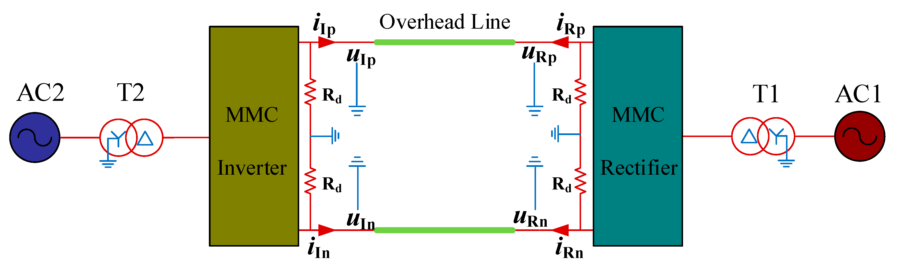
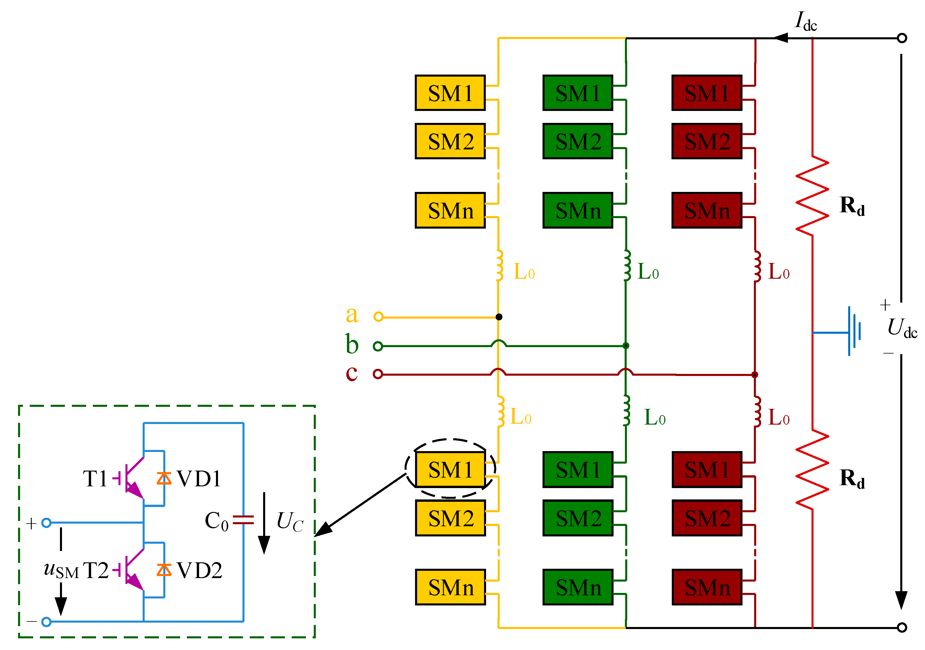
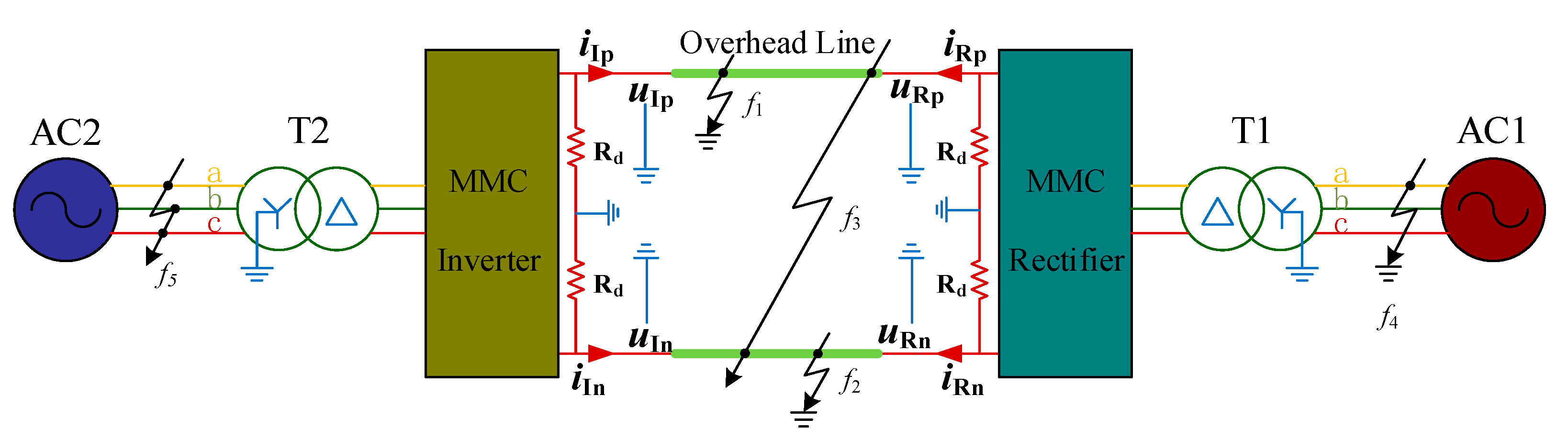
2. System Modelling of MMC-HVDC

An MMC-HVDC system [27] is mainly composed of MMC converter stations at both sides and DC transmission lines. The structure of MMC-HVDC system is shown in Figure 1. Here, alternating current (AC) systems at both converter stations are active networks, and the equivalent model of AC system with a rated voltage of 230 kV and frequency of 50 Hz is adopted. The winding of the valve side of the connecting transformer adopts triangle connection without neutral point, while the AC side of the connecting transformer adopts star connection and its neutral point is directly grounded. The DC side is grounded by the clamp resistance (R_d) whose resistance value is very large. The main function of the clamp resistance is to provide the voltage at both poles of the clamp and the potential reference point of the DC system during normal operations. The rated DC voltage is ±320 kV, the transmission line is 400 km, and the rated power is 1200 MVA. Four observation points are set on the MMC-HVDC system at the rectifier and inverter. The corresponding voltage and current can be measured at the observation point. u_Rp and u_Rn are, respectively, the positive and negative voltage on the rectifier side, and u_Ip and u_In are, respectively, the positive and negative voltage on the inverter side. i_Rp and i_Rn are positive and negative currents on the rectifier side, while i_Ip and i_In are positive and negative currents on the inverter side. The reference direction of the current is shown in Figure 1. The circuit diagram of a symmetrical MMC and the structure of one sub-module are shown in Figure 2. The arm inductances and sub-module capacitances of each MMC are La = 50 mH and C = 2800 μF, respectively.

3. Single Pole-to-Ground Fault Analysis

In the MMC-HVDC system shown in Figure 1, the DC side bus is grounded by clamping resistance. Since the DC side is grounded by two large resistors, the DC voltage at both poles is clamped to provide potential reference points for the DC system. As the DC valve sides at both ends are triangular wiring, when a single pole-to-ground fault occurs in the MMC-HVDC system, there is no connection point to the ground. Additionally, the clamping resistance on the DC side has a large resistance value, which can be approximately regarded as open circuit when single pole-to-ground fault occurs. For the AC side, only the potential reference point of the DC system is changed theoretically, while the DC system can still transmit power. For DC transmission lines, after steady state, the fault pole voltage is reduced to 0, the other pole voltage is clamped to the double, and the interpole voltage U_dc remains unchanged. Therefore, the insulation level of non-fault pole is required to be higher, and the transmission system should diagnose the single pole-to-ground fault in time.

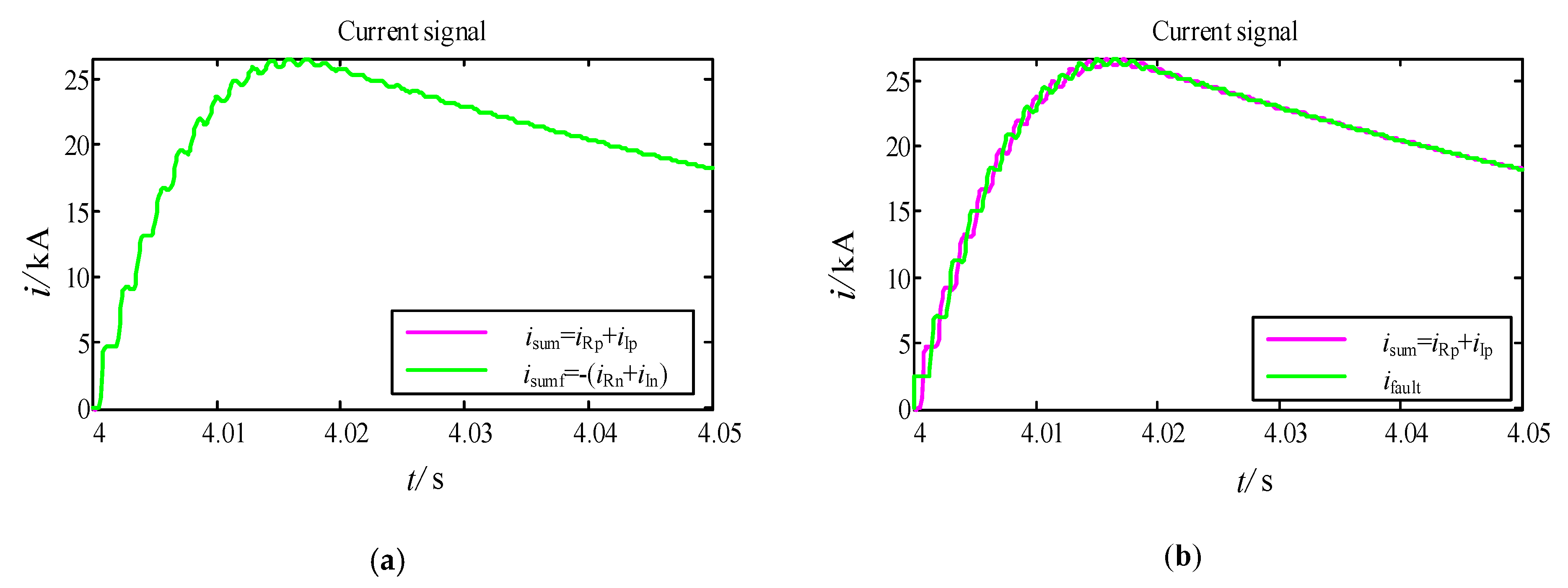
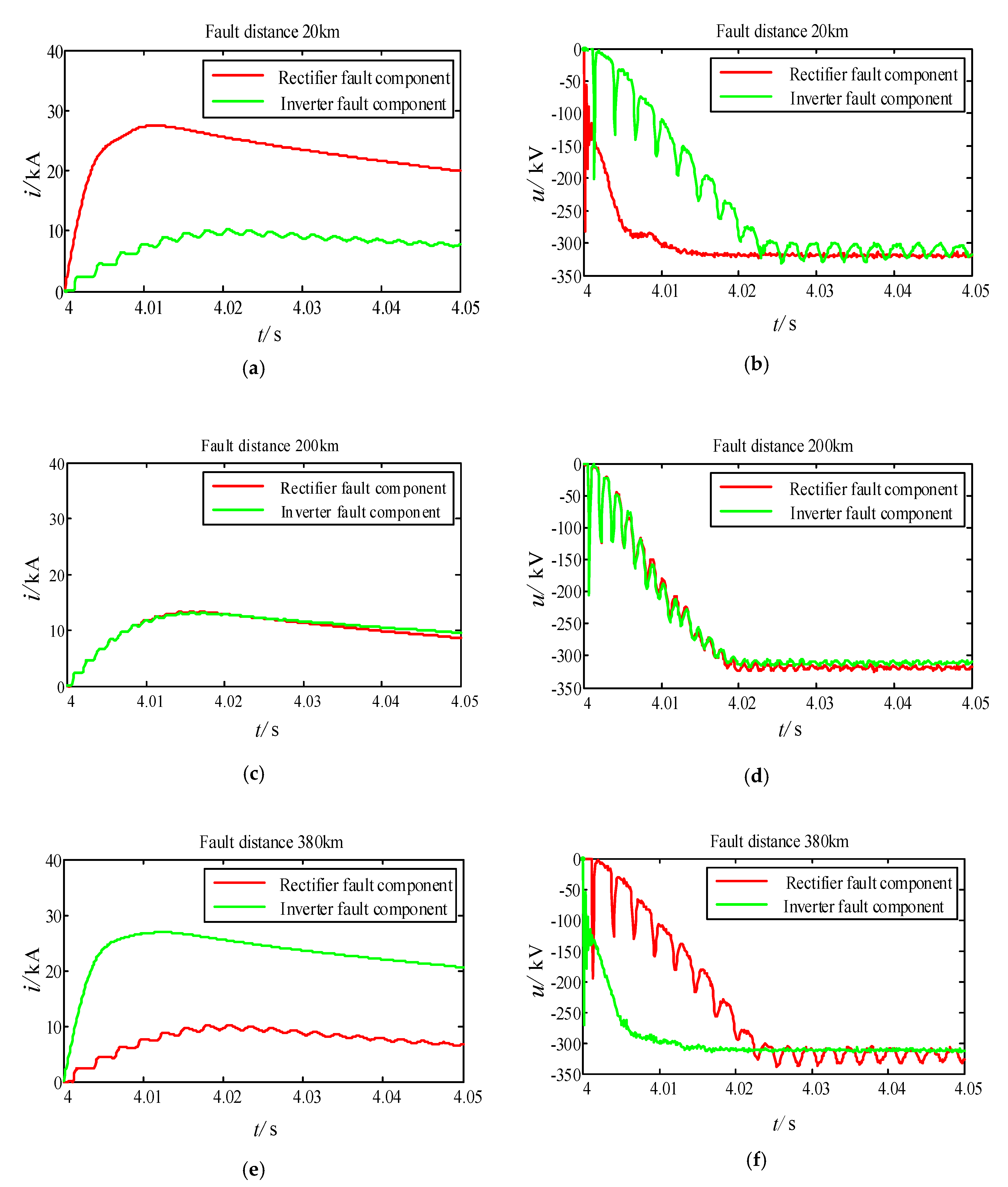
3.1. Transient Process after Single Pole-to-Ground Fault

If the system has a pole-to-ground fault at the positive pole line f₁, due to the distributed capacitance of the transmission line, after the fault pole is grounded by the resistance R_f, the distributed capacitance of the non-fault pole and the fault pole will form a path for the fault transient current illustrated in Figure 3. The simulation results show that the current flowing from the fault point to the negative electrode line coincides with the current flowing from the positive electrode line to the fault point, which is consistent with the theoretical results. The fault current comparison is shown in Figure 4. The current observed in the positive electrode line at the rectifier side and the inverter side is basically consistent with the current measured at the fault point, while the fault current is slightly greater than the sum of the current measured at both ends. This is because the inter-electrode distributed capacitance conduction provides a path for part of the fault current, which does not pass through the measuring points at both ends.

The magnitude of the current i₁ and i₂ in the two circuits is related to the impedance of the circuit at both ends, while the impedance of the circuit is related to the length of the circuit: the longer the line is, the greater of the impedance and smaller of the shunt will be. In this paper, the fault distance refers to the distance from the fault point to the rectifier side. A closer fault distance means a smaller line impedance. Compared with i₂, the amplitude of i₁ is larger and the oscillation is more obvious. When the fault occurs in the middle of the line, the line impedance at both ends is the same, that is, i₁ is almost equal to i₂. The fault components of the current and voltage on the rectifier side and the inverter side are compared in Figure 5, in which the fault distances are 20, 200, and 380 km, respectively.

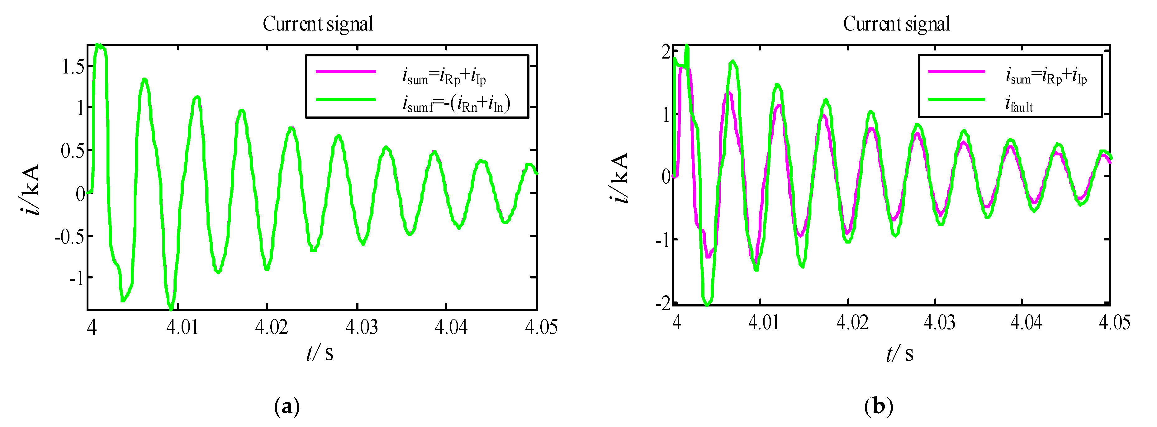
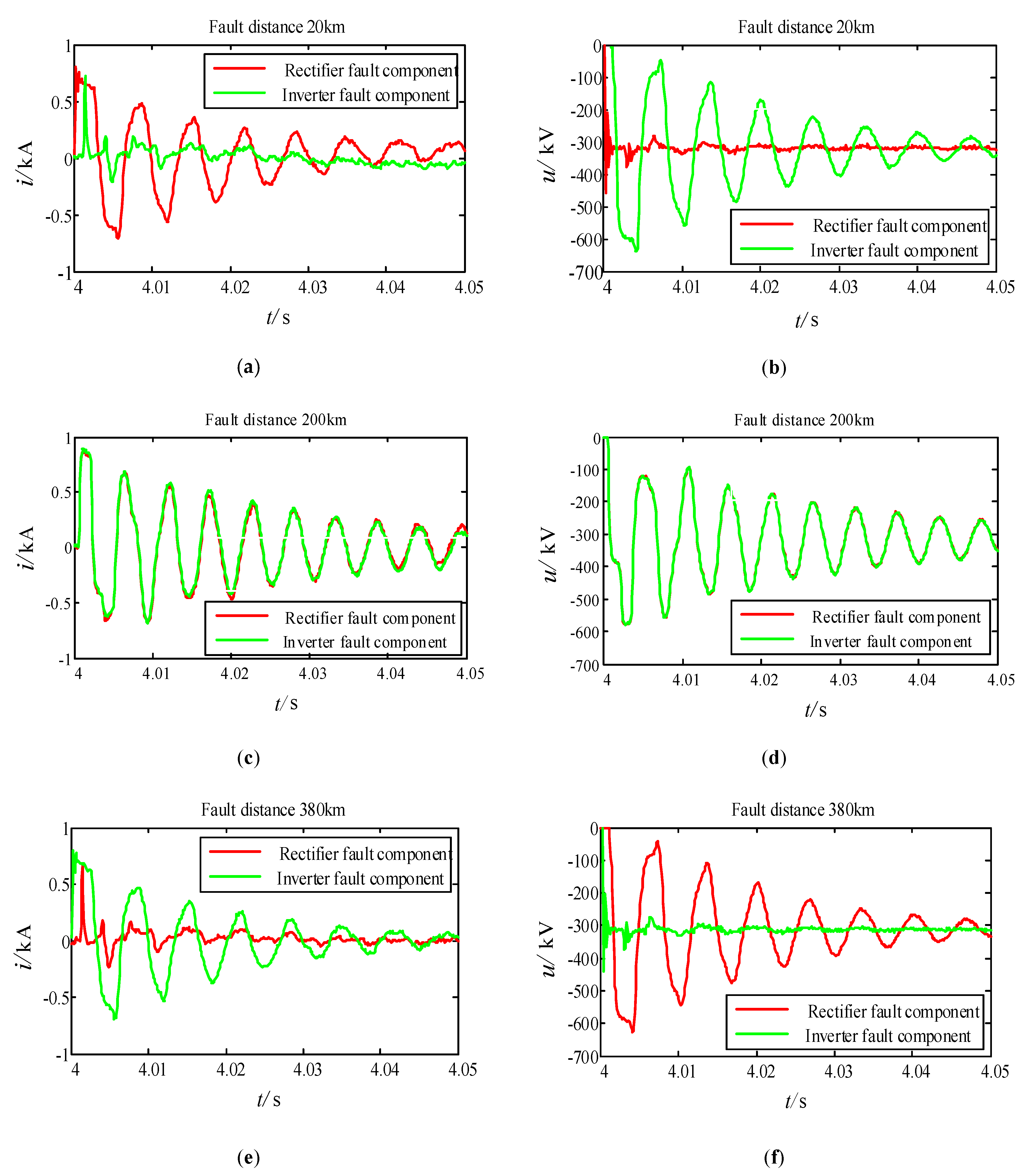
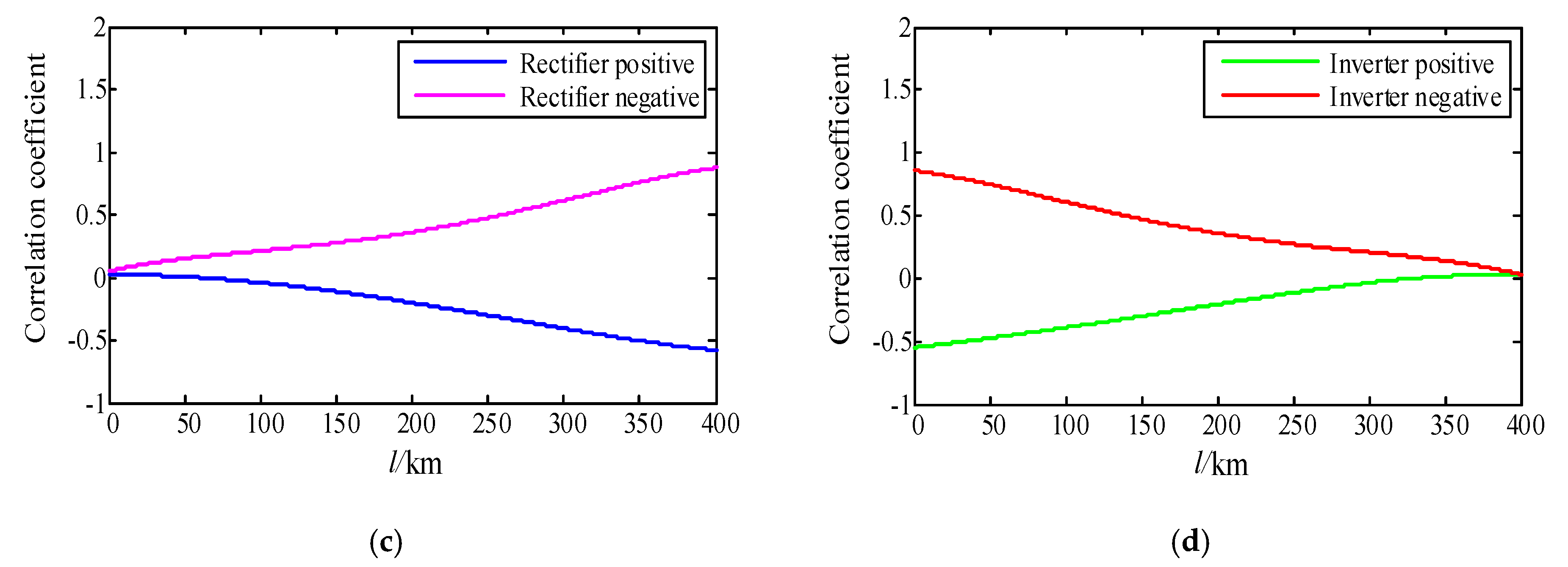
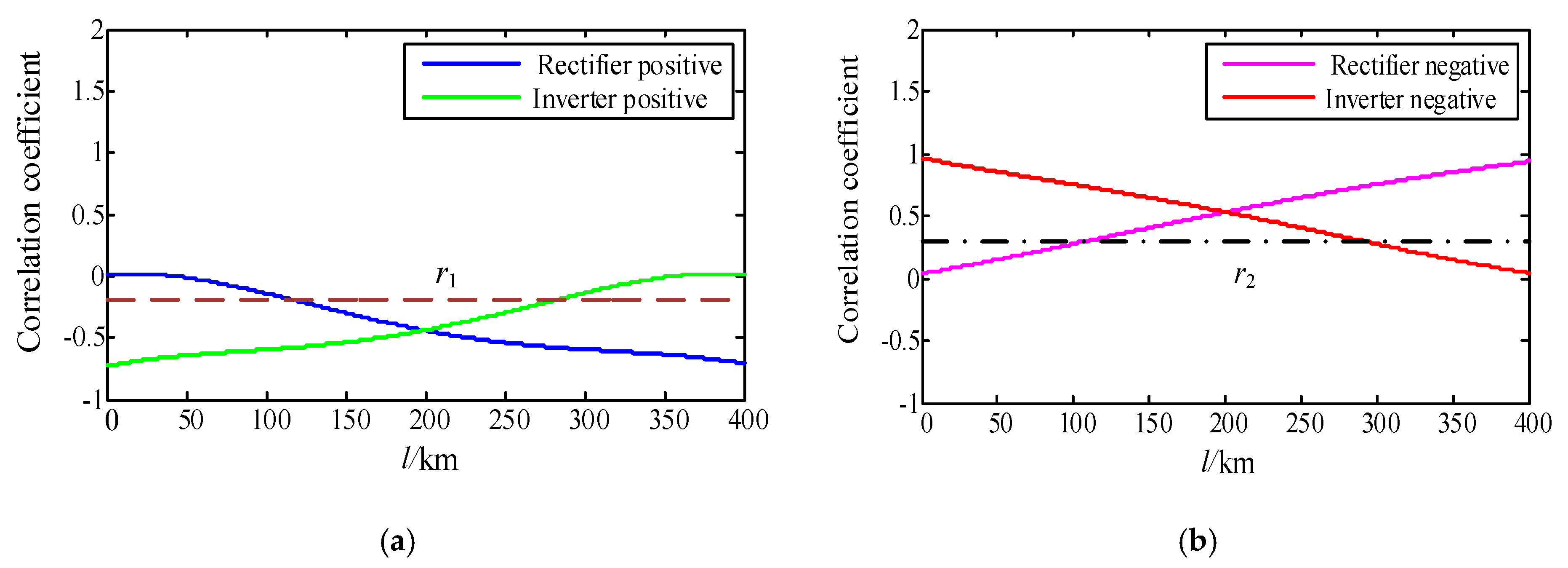
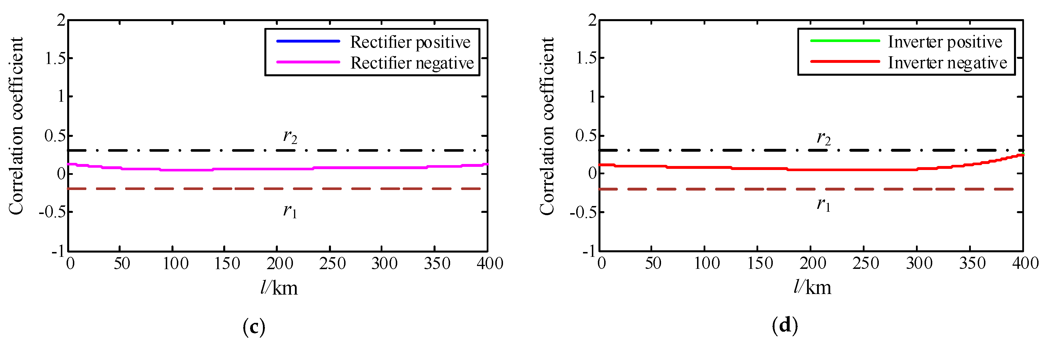
3.2. Correlation Analysis of Single Pole-to-Ground Fault

The transient process of MMC-HVDC system after a single pole-to-ground fault is the discharge process of line distributed capacitance. From Equation (1), it can be seen from the relation of voltage and current of capacitor element that if the relationship of the current and voltage change rate is proportional, the element is considered to be capacitive [28]. For the transmission line, it is actually a complex RLC circuit with both capacitive and inductive characteristics. That mean the transmission line is a second order system, which is shown in Figure 5. This paper analyzes and describes the difference between a single pole-to-ground fault and other types of fault from the perspective of capacitive characteristics. The correlation coefficient between voltage change rate and current is proposed to characterize the capacitive characteristics of the observation point after failure.

$$i=C\frac{\mathrm{d}u}{\mathrm{d}t}.$$

(1)

The correlation coefficient of Pearson is to measure the correlation degree of two variables by using covariance and variance, which is not affected by the amplitude of variables [29]. The correlation coefficient of Pearson can effectively measure the similarity of two different variables, and the discrete expression of the correlation coefficient is described as

$$\rho (\mathrm{d}u/\mathrm{d}t,i)=\rho (x,y)=\frac{{\displaystyle \sum _{k=1}^n(x_k}-\frac{1}{n}{\displaystyle \sum _{j=1}^n{x}_j)}(y_k-\frac{1}{n}{\displaystyle \sum _{j=1}^n{y}_j)}}{\sqrt{{\displaystyle \sum _{k=1}^n(x_k}-\frac{1}{n}{\displaystyle \sum _{j=1}^n{x}_j{)}^2}}\sqrt{{\displaystyle \sum _{k=1}^n(y_k}-\frac{1}{n}{\displaystyle \sum _{j=1}^n{y}_j{)}^2}}}$$

(2)

where x and y are two different variables, $x=\{x_1,x_2,\dots ,x_n\}$, $y=\{y_1,y_2,\dots ,y_n\}$, and n are the sampling points. Variable $\mathrm{d}u/\mathrm{d}t$ is equivalent to x, and variable i is equivalent to y.

Here, $r=\rho (\mathrm{d}u/\mathrm{d}t,i)=1$ indicates that the change rules of the two variables $\mathrm{d}u/\mathrm{d}t$ and i are exactly the same, e.g., the correlation is the strongest and the two waveforms represented are completely similar. Meanwhile, $r=\rho (\mathrm{d}u/\mathrm{d}t,i)=-1$ indicates that the change rules of two variables $\mathrm{d}u/\mathrm{d}t$ and i are completely opposite, e.g., the strongest correlation is negative. The two waveforms represented are axisymmetric and completely similar as negative. When the absolute value of r is close to zero, it indicates that the variation rules of the two variables are significantly different, e.g., the correlation is extremely weak and the similarity of the two waveforms represented is extremely low.

For pole-to-ground faults, the correlation between the voltage change rate and the current at the measurement point is related to the internal structure of the MMC and the length of the transmission line. For the studied system, the internal structure of the MMC has been determined. The variation of the correlation coefficient $\rho (\mathrm{d}u/\mathrm{d}t,i)$ between the voltage change rate and the current at the measurement point is mainly related to the line length: the longer the transmission line, the greater the distributed capacitance between the poles, and the greater the correlation coefficient between the voltage change rate and the current obtained at the measurement point.

The positive pole-to-ground fault of the transmission line is simulated through the whole line to obtain the correlation coefficient between voltage change rate and current at different fault locations, as shown in Figure 6 and Figure 7. One can observe that the correlation coefficients between the voltage change rate and current of the positive pole on the rectifier side and the inverter side are compared, as well as the correlation coefficients of the negative pole. Similarly, the correlation coefficients of the positive and negative pole on the rectifier side and the correlation coefficients of the positive and negative pole on the inverter side are compared, respectively, as well as the correlation coefficients of two different transition resistances.

As it can be seen from Figure 6 and Figure 7, in the case of proximal fault (the fault is close to the rectifier side), the correlation coefficient between the voltage change rate and the current of the positive pole line on the rectifier side is close to zero. With the increase of fault distance, the correlation between positive line voltage change rate and current increases, and the absolute value of correlation coefficient increases, but it is negative, indicating that the negative correlation is gradually increasing. The correlation coefficient between the voltage change rate and the current of the negative line on the rectifier side is also close to zero when the proximal fault occurs. With the increase of the fault distance, the correlation between the negative line voltage change rate and the current increases and it is positive. The absolute value of the correlation coefficient increases. The correlation between the voltage change rate and the current on the inverter side is opposite to that on the rectifier side. When the proximal side of the rectifier fails, the correlation coefficient between the voltage change rate and the current on the positive side of the inverter side is the most negative, showing a strong negative correlation. With the increase of fault distance, the absolute value of correlation coefficient decreases, and the negative correlation weakens. The correlation coefficient between the negative line voltage change rate and the current on the inverter side is the positive maximum value in the case of proximal fault (the fault is close to the rectifier side), showing a positive strong correlation. With the increase of fault distance, the absolute value of correlation coefficient decreases, and the positive correlation weakens. Moreover, the correlation coefficient between the voltage change rate and the current at the same positive and negative observation points is roughly one positive and one negative.

When the positive pole-to-ground fault occurs on the transmission line, for the positive electrode line, the correlation coefficient ${\rho }_{j\mathrm{p}}=\rho (\mathrm{d}{u}_{j\mathrm{p}}/\mathrm{d}t,i_{j\mathrm{p}})$ (j = R or j = I) between the voltage change rate and the current obtained from the two observation points on the rectifier side or the inverter side is less than or equal to certain value r₁ (−1 < r₁ < 0), giving

$$\min ({\rho }_{\mathrm{Rp}},{\rho }_{\mathrm{Ip}})\le r_1.$$

(3)

If the correlation coefficient of the rectifier side is greater than r₁ and close to zero, while the correlation coefficient of the inverter side is less than r₁, the fault location is closer to the rectifier side. If the correlation coefficients of the rectifier side and the inverter side are less than r₁, the fault location is located in the middle of the transmission line. If the correlation coefficient of the rectifier side is less than r₁, while the correlation coefficient of the inverter side is greater than r₁ and close to zero, the fault location is closer to the inverter side.

When the positive pole-to-ground fault occurs on the transmission line, for the negative line, the correlation coefficient between the voltage change rate and the current obtained from two observation points on the rectifier side or the inverter side is greater than or equal to certain value r₂ (0 < r₂ < 1), yielding

$$\max ({\rho }_{\mathrm{Rn}},{\rho }_{\mathrm{In}})\ge r_2.$$

(4)

If the correlation coefficient of the rectifier side is less than r₂ and close to zero, while that of the inverter side is greater than r₂, the fault location is closer to the rectifier side. If the correlation coefficients of the rectifier side and the inverter side are greater than r₂, the fault location is located in the middle of the transmission line. If the correlation coefficient of the rectifier side is greater than r₂, while that of the inverting side is less than r₂ and close to zero, the fault location is closer to the inverter side. The correlation coefficients with the reference value is shown in Figure 8.

It can also be found from the above analysis that when the transmission line has a single pole-to-ground fault, the fault can be identified by combining the information of the observation points of the fault pole and the non-fault pole. Additionally, the correlation coefficients of the fault pole and non-fault pole are positive and negative. The correlation coefficient between voltage change rate and current of the fault pole is mainly negative, while the correlation coefficient of the non-fault pole is mainly positive. In addition, the absolute value of the correlation coefficient of the non-fault pole is slightly larger than that of the fault pole. Therefore, the correlation coefficient between voltage change rate and current can be obtained from the four observation points at both ends of the transmission line, so that the fault line can be determined and the approximate location of the fault (proximal, intermediate, or distal) can be diagnosed.

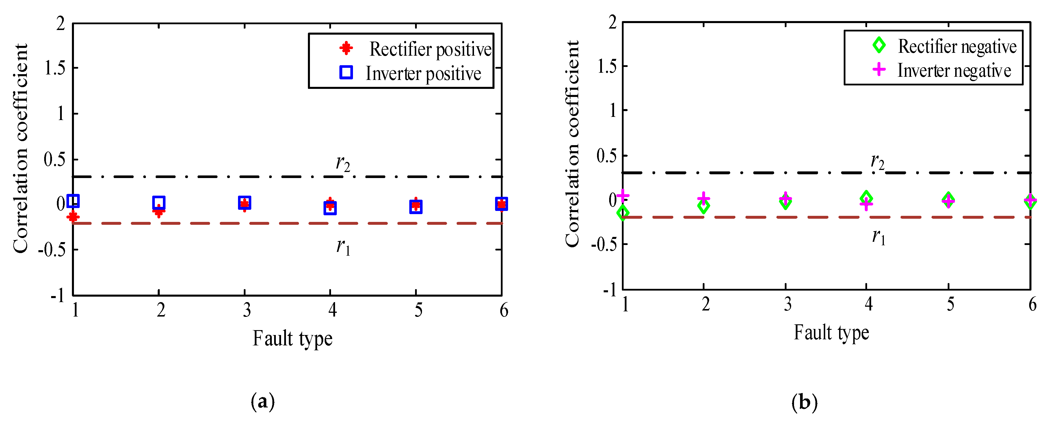
4. Analysis of Other Faults

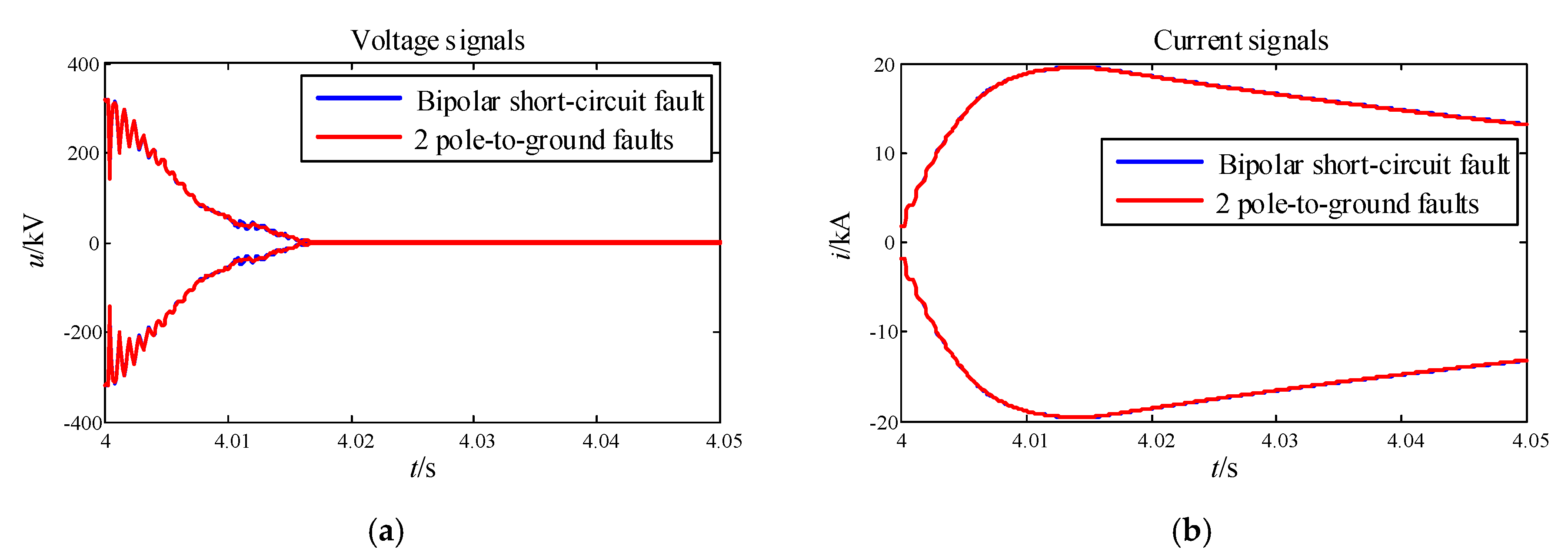
4.1. Bipolar Short-Circuit Fault

After a bipolar short-circuit fault occurs in the MMC-HVDC transmission line, both the positive and negative voltage of the DC transmission line and the inter-electrode voltage drop, and the amplitude of the decline is related to the transition resistance. In the event of a metallic bipolar short-circuit fault, the voltage amplitude of the transmission line falls to zero. The transient process of a bipolar short-circuit fault in DC transmission lines is also very different from that of a single pole-to-ground fault. The fault current calculated at both ends after the bipolar short-circuit fault and that measured at the fault point are compared in Figure 9. It can be seen that the two currents are basically identical, with little difference in value, which is quite different from the single pole-to-ground fault. The calculated value of the current at both ends of the single pole-to-ground fault is significantly less than the value measured at the fault point. This indicates that there is no obvious discharge process in the distributed capacitance of the bipolar line during the transient process of the bipolar short-circuit fault, which is essentially different from the single pole-to-ground fault. Figure 10 shows the current fault component and the voltage fault component of the rectifier side and the inverter side in the fault distances of 20, 200, and 380 km, respectively. It can be seen that the fault component of the proximal current has a large shunt.

If there are two pole-to-ground faults happening at the same time, it is a bipolar short-circuit fault for the MMC-HVDC system. Unlike a bipolar short-circuit fault, the current flow path of two pole-to-ground faults must be pole-to-ground-to-pole. The voltage and current of the two scenarios are compared in Figure 11. The voltage and current under two pole-to-ground faults that happened at the same time are basically consistent with the bipolar short-circuit fault.

When a bipolar short-circuit fault occurs, the distributed capacitance between the poles of the transmission line is equivalent to being short-connected, and the correlation between the voltage change rate and the current obtained at the measurement point is weak with a small correlation coefficient $\rho (\mathrm{d}u/\mathrm{d}t,i)$. The correlation coefficients between the voltage change rate and the current of the bipolar short-circuit fault are shown in Figure 12. When the bipolar short-circuit fault occurs, both for positive and negative lines, the correlation coefficients between the voltage change rate and the corresponding current obtained from the two observation points on the rectifier side and the inverter side are both greater than a certain value r₁ (−1 < r₁ < 0), and less than a certain value r₂ (0 < r₂ < 1). This can be expressed as follows

$$r_1<{\rho }_{\mathrm{R}i},{\rho }_{\mathrm{I}i}<r_2,$$

(5)

where i = p, or I = n, ${\rho }_{\mathrm{R}i}$ represents the correlation coefficient of positive or negative circuits on the rectifier side, and ${\rho }_{\mathrm{I}i}$ represents the correlation coefficient of positive or negative circuits on the inverter side.

In other words, when the bipolar short-circuit fault occurs, the correlation coefficient between the voltage change rate and corresponding current obtained from the four observation points at both ends of the transmission line are between the two fixed values.

4.2. AC Side Fault

In the case of an AC side fault, the correlation between voltage change rate and current obtained from observation points at both ends is related to the MMC-HVDC system, and the correlation between voltage change rate and current is very weak. Figure 13 shows the correlation coefficient between the voltage change rates and the current when the AC side fails. Here, 1 is single-phase grounding fault (A-G) on the rectifier side, 2 is two-phase grounding fault (AB-G) on the rectifier side, 3 is three-phase short-circuit fault (ABC) on the rectifier side, 4 is single-phase grounding fault (A-G) on the inverter side, 5 is two-phase grounding fault (AB-G) on the inverter side, and 6 is three-phase short-circuit fault (ABC) on the inverter side. When an AC side fault occurs, for the positive line, the correlation coefficient between the voltage change rate and the corresponding current obtained from the two observation points on the rectifier side and the inverter side are both greater than a certain value r₁ (−1 < r₁ < 0), and less than a certain value r₂ (0 < r₂ < 1). For the negative line, the correlation coefficient between the voltage change rate and the corresponding current obtained from the two observation points on the rectifier side and the inverter side are both greater than a certain value r₁ (−1 < r₁ < 0), and less than a certain value r₂ (0 < r₂ < 1). In other words, when an AC side fault occurs, the correlation coefficient between the voltage change rate and corresponding current obtained from the four observation points at both ends of the transmission line are between the two fixed values, which also satisfies Equation (5).

5. Capacitive Fuzzy Identification of a Single Pole-to-Ground Fault

5.1. Capacitive Fuzzy Recognition Algorithm

In general, for the single pole-to-ground fault of MMC-HVDC transmission line, the correlation coefficient between voltage change rate and current of the fault pole is mainly negative, while the correlation coefficient of the non-fault pole is mainly positive. Additionally, the absolute value of the correlation coefficient of the non-fault pole is slightly larger than that of the fault pole. For the fault line, the correlation coefficient between the voltage change rate and the current obtained from two observation points on the rectifier side or the inverter side is less than a certain value r₁ (−1 < r₁ < 0). For the non-fault line, the correlation coefficient between the voltage change rate and the current obtained from two observation points on the rectifier side or the inverter side is greater than a certain value r₂ (0 < r₂ < 1). The correlation coefficients between the voltage change rate and the current at the same positive and negative observation points are generally one positive and one negative.

When other faults occur in MMC-HVDC systems, the correlation between the voltage change rate and the current is very weak. The correlation coefficient between the voltage change rate and the current at the positive pole is consistent with the symbol of the correlation coefficient at the negative pole, and the absolute values of the correlation coefficients are also very close.

Let ${\rho }_{j\mathrm{p}}=\rho (\mathrm{d}{u}_{j\mathrm{p}}/\mathrm{d}t,i_{j\mathrm{p}})$ (j = R or j = I) be the correlation coefficient of the positive line voltage change rate and current on the rectifier or inverter side, and let ${\rho }_{j\mathrm{n}}=\rho (\mathrm{d}{u}_{j\mathrm{n}}/\mathrm{d}t,i_{j\mathrm{n}})$ (j = R or j = I) be the correlation coefficient between the negative line voltage change rate and current on the rectifier or inverter side, then the ratio K_j (j = R or j = I) is

$$K_j=\frac{{\rho }_{j\mathrm{p}}}{{\rho }_{j\mathrm{n}}}=\frac{\rho (\mathrm{d}{u}_{j\mathrm{p}}/\mathrm{d}t,i_{j\mathrm{p}})}{\rho (\mathrm{d}{u}_{j\mathrm{n}}/\mathrm{d}t,i_{j\mathrm{n}})}.$$

(6)

According to the characteristics of an MMC-HVDC transmission line after a single pole-to-ground fault, K_j should be negative, while K_j should be positive when other faults occur.

When the near-end single pole-to-ground fault occurs (assume in the rectifier side), the correlation between the voltage change rate and the current is relatively weak, and the corresponding correlation coefficient is near zero. Due to factors such as measurement error and calculation error, the ratio of K_R may be positive. However, for the other end, it is the fault of the remote end. The correlation between the voltage change rate and the current is very strong, and the corresponding correlation coefficient is also relatively high. The ratio K_I must be negative. Therefore, if only one ratio K_j is negative, a single pole-to-ground fault can be determined. It can also be expressed that as long as the small K_j value is negative, it can be determined as a single pole-to-ground fault, which gives

min(K_R,K_I) < 0.

(7)

It can be seen from the previous analysis that the absolute value of the voltage change rate and current correlation coefficient of the fault pole is slightly less than that of the non-fault pole when the single pole-to-ground fault occurs. K_j is the correlation coefficient of the positive line divided by the correlation coefficient of the negative line. In case of the positive pole-to-ground fault, the correlation coefficient ${\rho }_{j\mathrm{p}}$ of the positive pole is slightly less than that of negative pole ${\rho }_{j\mathrm{n}}$. Therefore, |K_j| is less than 1. If the negative pole-to-ground fault occurs, the positive line correlation coefficient ${\rho }_{j\mathrm{p}}$ is slightly greater than the negative line correlation coefficient ${\rho }_{j\mathrm{n}}$, so |K_j| is greater than 1, as follows

$$\{\begin{array}{l}\left|K_{\mathrm{R}}\right|<1,\left|K_{\mathrm{I}}\right|<1,\mathrm{Positive}\mathrm{pole}-\mathrm{to}-\mathrm{ground}\mathrm{fault}\\ \left|K_{\mathrm{R}}\right|<1,\left|K_{\mathrm{I}}\right|<1,\mathrm{Negative}\mathrm{pole}-\mathrm{to}-\mathrm{ground}\mathrm{fault}\end{array}.$$

(8)

Note that the above method is called capacitive fuzzy recognition because it derives from the capacitive characteristics of the line measured according to the correlation.

5.2. Fault Identification Flow Chart

From the aforementioned analysis, the correlation coefficient ratio between positive and negative in the case of a single pole-to-ground fault in MMC-HVDC transmission lines, K_j, is quite different from the correlation coefficient ratio calculated in other types of faults. The ratio K_j of the rectifier side and the inverter side is calculated respectively. According to Equation (7), it is determined whether the MMC-HVDC transmission line has a single pole-to-ground fault. If a single pole-to-ground fault occurs, the fault pole can be identified according to Equation (8). The single pole-to-ground fault identification process is demonstrated in Figure 14.

5.3. Quantitative Simulation Results

The studied MMC-HVDC system is built on PSCAD4.5 version via a personal computer with an IntelR CoreTMi5 CPU at 3.2 GHz and 12 GB of RAM. The fault setting points are shown in Figure 15. For the single pole-to-ground fault on the DC side, positive pole-to-ground fault (f₁) and negative pole-to-ground fault (f₂) are set at different positions. For other faults, the bipolar short-circuit fault (f₃), the single-phase grounding fault (A-G) on the AC side of the rectifier (f₄), and the three-phase short-circuit fault (ABC) on the AC side of the inverter (f₅) are set. When a fault occurs in the MMC-HVDC system, the capacitive fuzzy recognition algorithm is applied to identify the single pole-to-ground fault of MMC-HVDC transmission line. According to Equation (7), it is determined whether the MMC-HVDC transmission line has a single pole-to-ground fault. If a single pole-to-ground fault occurs, the fault pole can be identified according to Equation (8). The quantitative simulation results are provided in

Table 1. Results of fault type.

Fault Types	Fault Distance (km)	Fault Resistance (Ω)	KR	KI	Min (KR, KI) < 0	Result
f1	20	0.01	0.679	−0.751	Y	Single pole-to-ground fault
f1	60	0.01	−0.168	−0.744	Y	Single pole-to-ground fault
f1	140	100	−0.295	−0.683	Y	Single pole-to-ground fault
f1	180	0.01	−0.735	−0.858	Y	Single pole-to-ground fault
f1	260	100	−0.698	−0.294	Y	Single pole-to-ground fault
f1	320	0.01	−0.799	−0.461	Y	Single pole-to-ground fault
f2	90	0.01	−2.230	−1.302	Y	Single pole-to-ground fault
f2	190	0.01	−1.201	−1.159	Y	Single pole-to-ground fault
f2	360	0.01	−1.344	−8.442	Y	Single pole-to-ground fault
f3	100	100	1.000	1.000	N	Other faults
f3	150	0.01	0.998	1.000	N	Other faults
f3	300	0.01	1.000	1.000	N	Other faults
f4	--	0.01	0.999	1.000	N	Other faults
f5	--	0.01	1.006	1.000	N	Other faults

and

Table 2. Results of fault pole.

Fault Types	Fault Distance (km)	Fault Resistance (Ω)	KR	KI	|KR| < 1, |KI| < 1	|KR| > 1, |KI| > 1	Result
f1	20	0.01	0.679	−0.751	Y	N	Positive pole-to-ground fault
f1	60	0.01	−0.168	−0.744	Y	N	Positive pole-to-ground fault
f1	140	100	−0.295	−0.683	Y	N	Positive pole-to-ground fault
f1	180	0.01	−0.735	−0.858	Y	N	Positive pole-to-ground fault
f1	260	100	−0.698	−0.294	Y	N	Positive pole-to-ground fault
f1	320	0.01	−0.799	−0.461	Y	N	Positive pole-to-ground fault
f2	90	0.01	−2.230	−1.302	N	Y	Negative pole-to-ground fault
f2	190	0.01	−1.201	−1.159	N	Y	Negative pole-to-ground fault
f2	360	0.01	−1.344	−8.442	N	Y	Negative pole-to-ground fault

, respectively, considering different fault distance, faulty poles, and fault resistance.

In Table 1, the positive pole-to-ground fault and the negative pole-to-ground fault are correctly identified as a single pole-to-ground fault by using Equation (7), and the bipolar short-circuit fault and AC side faults are other faults. For the single pole-to-ground faults, the fault poles are identified correctly according to Equation (8). The results are presented in Table 2.

6. Conclusions

This paper presents a novel capacitive fuzzy identification algorithm based on the characteristics of a single pole-to-ground fault in MMC-HVDC transmission lines. After the single pole-to-ground fault of the MMC-HVDC transmission line occurs, the correlation coefficient between the voltage change rate and the current of the fault pole is mainly negative, while the correlation coefficient of the non-fault pole is mainly positive. Additionally, the absolute value of the correlation coefficient of the non-fault pole is slightly larger than that of the fault pole. However, other types of failures have no such characteristics.

In the proposed algorithm, the ratio of correlation coefficients (K_j) is calculated by the rectifier side and the inverter side, respectively. As long as K_j is negative on one side, it can be determined that the MMC-HVDC transmission line has a single pole-to-ground fault. Based on the value of |K_j|, whether it is less or greater than 1, the fault pole can be identified.

When the single pole-to-ground fault occurs in the MMC-HVDC transmission line, the approximate location of the fault (proximal, intermediate, and distal) can be roughly determined from both the fault pole and non-fault pole. For the fault line, if the correlation coefficient of the rectifier side is greater than r₁ and close to zero, while the correlation coefficient of the inverter side is less than r₁, the fault location is closer to the rectifier side. On the other hand, if the correlation coefficients of both the rectifier side and the inverter side are less than r₁, the fault location is located in the middle of the transmission line. Moreover, if the correlation coefficient of the rectifier side is less than r₁, while the correlation coefficient of the inverter side is greater than r₁ and close to zero, the fault location is closer to the inverter side.

References

1. Yang, B.; Yu, T.; Shu, H.C.; Dong, J.; Jiang, L. Robust sliding-mode control of wind energy conversion systems for optimal power extraction via nonlinear perturbation observers. Appl. Energy 2018, 210, 711–723. [Google Scholar] [CrossRef]
2. Yang, B.; Yu, T.; Shu, H.C.; Zhang, Y.M.; Chen, J.; Sang, Y.Y.; Jiang, L. Passivity-based sliding-mode control design for optimal power extraction of a PMSG based variable speed wind turbine. Renew. Energy 2018, 119, 577–589. [Google Scholar] [CrossRef]
3. Yang, B.; Jiang, L.; Wang, L.; Yao, W.; Wu, Q.H. Nonlinear maximum power point tracking control and model analysis of DFIG based wind turbine. Int. J. Electr. Power Energy Syst. 2016, 74, 429–436. [Google Scholar] [CrossRef] [Green Version]
4. Yang, B.; Zhang, X.S.; Yu, T.; Shu, H.C.; Fang, Z.H. Grouped grey wolf optimizer for maximum power point tracking of doubly-fed induction generator based wind turbine. Energy Convers. Manag. 2017, 133, 427–443. [Google Scholar]
5. Yang, B.; Yu, T.; Zhang, X.S.; Li, H.F.; Shu, H.C.; Sang, Y.Y.; Jiang, L. Dynamic leader based collective intelligence for maximum power point tracking of PV systems affected by partial shading condition. Energy Convers. Manag. 2019, 179, 286–303. [Google Scholar] [CrossRef]
6. Yang, B.; Yu, T.; Shu, H.C.; Qu, K.P.; Jiang, L. Democratic joint operations algorithm for optimal power extraction of PMSG based wind energy conversion system. Energy Convers. Manag. 2018, 159, 312–326. [Google Scholar] [CrossRef]
7. Andersen, B.R.; Xu, L. Hybrid HVDC system for power transmission to island networks. IEEE Trans. Power Deliv. 2004, 19, 1884–1890. [Google Scholar] [CrossRef]
8. O’Reilly, J.; Wood, A.R.; Osauskas, C.M. Frequency domain based control design for an HVDC converter connected to a weak AC network. IEEE Trans. Power Deliv. 2003, 18, 1028–1033. [Google Scholar] [CrossRef]
9. Thallam, R.S.; Mogri, S.; Burton, R.S. Harmonic impedance and harmonic interaction of an AC system with multiple DC infeeds. IEEE Trans. Power Deliv. 1988, 3, 2064–2071. [Google Scholar] [CrossRef]
10. Zheng, X.D.; Tai, N.L.; Thorp, J.S.; Yang, G.L. A transient harmonic current protection scheme for HVDC transmission line. IEEE Trans. Power Deliv. 2012, 27, 2278–2285. [Google Scholar] [CrossRef]
11. Long, W.; Nilsson, S. HVDC transmission: Yesterday and today. IEEE Power Energy Mag. 2007, 2, 22–31. [Google Scholar] [CrossRef]
12. Bi, T.S.; Wang, S.; Jia, K. Single pole-to-ground fault location method for MMC-HVDC system using active pulse. IET Gener. Transm. Distrib. 2018, 12, 272–278. [Google Scholar] [CrossRef]
13. Adam, G.P.; Ahmed, K.H.; Finney, S.J.; Bell, K.R. New breed of network fault tolerant voltage source converter HVDC transmission system. IEEE Trans. Power Syst. 2012, 28, 335–346. [Google Scholar] [CrossRef]
14. Trainer, D.R.; Davidson, C.C.; Oates, C.D.M.; Macleod, N.M.; Critchley, D.R.; Crookes, R.W. A new hybrid voltage sourced converter for HVDC power transmission. CIGRE 2010, 2010, 1–12. [Google Scholar]
15. Xu, Y.; Liu, J.Y.; Fu, Y. Fault-line selection and fault-type recognition in DC systems based on graph theory. Prot. Control. Mod. Power Syst. 2018, 3, 267–276. [Google Scholar] [CrossRef]
16. Li, B.; He, J.W.; Li, Y.; Li, B.T. A review of the protection for the multi-terminal VSC-HVDC grid. Prot. Control. Mod. Power Syst. 2019, 4, 239–249. [Google Scholar] [CrossRef]
17. Musa, M.H.H.; He, Z.Y.; Fu, L.; Deng, Y.J. A cumulative standard deviation sum based method for high resistance fault identification and classification in power transmission lines. Prot. Control. Mod. Power Syst. 2018, 3, 291–302. [Google Scholar] [CrossRef] [Green Version]
18. Fan, W.; Liao, Y. Wide area measurements based fault detection and location method for transmission lines. Prot. Control. Mod. Power Syst. 2019, 4, 53–64. [Google Scholar] [CrossRef]
19. Akhmatov, V.; Callavik, M.; Franck, C.M.; Rye, S.E. Technical guidelines and prestandardization work for first HVDC grids. IEEE Trans. Power Deliv. 2014, 29, 327–335. [Google Scholar] [CrossRef] [Green Version]
20. Flourentzou, N.; Agelidis, V.G.; Demetriades, G.D. VSC-based HVDC power transmission systems: An overview. IEEE Trans. Power Electron. 2009, 24, 592–602. [Google Scholar] [CrossRef]
21. Gemmell, B.; Dorn, J.; Retzmann, D.; Soerangr, D. Prospects of multilevel VSC technologies for power transmission. In Proceedings of the 2008 IEEE/PES Transmission and Distribution Conference and Exposition, Chicago, IL, USA, 21–24 April 2008; pp. 1–16. [Google Scholar]
22. Xu, T. Research on Modeling and Control Strategies of Modular Multi-Level VSC-HVDC System. Master’s Thesis, Shenyang University of Technology, Shengyang, China, 2017. [Google Scholar]
23. Ma, Y.Q.; Wang, W.A.; Zhang, J.; Tang, J.Z.; Ren, T. Analysis of MMC-HVDC transient response characteristic under typical disturbances. Proc. Chin. Soc. Univ. Electr. Power Syst. Its Autom. 2011, 23, 110–118. [Google Scholar]
24. Wang, X.; Ooi, B.T. High voltage direct current transmission system based on voltage source converters. In Proceedings of the 21st Annual IEEE Conference on Power Electronics Specialists, San Antonio, TX, USA, 4–6 May 1990; pp. 325–332. [Google Scholar]
25. Pereira, L.; Kosterev, D.; Davies, D.; Patterson, S. New thermal governor model selection and validation in the WECC. IEEE Trans. Power Syst. 2004, 19, 517–523. [Google Scholar] [CrossRef]
26. Rajaraman, P.; Sundaravaradan, N.A.; Mallikarjuna, B.; Reddy, J.B. Robust fault analysis in transmission lines using Synchrophasor measurements. Prot. Control. Mod. Power Syst. 2018, 3, 108–110. [Google Scholar]
27. Friedrich, K. Modern HVDC Plus application of VSC in Modular Multilevel Converter Topology. In Proceedings of the 2010 IEEE International Symposium on Industrial Electronics, Bari, Italy, 4–7 July 2010. [Google Scholar] [CrossRef]
28. Lee, J.; Kang, D.; Lee, J. A Study on the Improved Capacitor Voltage Balancing Method for Modular Multilevel Converter Based on Hardware-In-the-Loop Simulation. Electronics 2019, 8, 1070. [Google Scholar] [CrossRef] [Green Version]
29. Ahlgren, P.; Jarneving, B.; Rousseau, R. Requirements for a cocitation similarity measure, with special reference to Pearson’s correlation coefficient. J. Am. Soc. Inf. Sci. Technol. 2003, 54, 550–560. [Google Scholar] [CrossRef]
Figure 1. Schematic diagram of a modular multilevel converter high voltage direct current (MMC-HVDC) transmission system.
Energies 13 00319 g001
Figure 2. Circuit diagram of a symmetrical MMC.
Energies 13 00319 g002
Figure 3. Fault current diagram.
Energies 13 00319 g003
Figure 4. Fault current comparison. (a) Positive pole current (isum) and negative pole current (isumf). (b) Positive pole current (isum) and fault current in the fault location.
Energies 13 00319 g004
Figure 5. The fault components of the current and voltage. (a) The current fault component. (b) The voltage fault component. (c) The current fault component. (d) The voltage fault component. (e) The current fault component. (f) The voltage fault component.
Energies 13 00319 g005
Figure 6. The correlation coefficients with fault resistance of 0.01 Ω. (a) The correlation coefficients of the positive line. (b) The correlation coefficients of the negative line. (c) The correlation coefficients on the rectifier side. (d) The correlation coefficients on the inverter side.
Energies 13 00319 g006
Figure 7. The correlation coefficients with fault resistance of 100 Ω. (a) The correlation coefficients of the positive line. (b)The correlation coefficients of the negative line. (c) The correlation coefficients on the rectifier side. (d) The correlation coefficients on the inverter side.
Energies 13 00319 g007aEnergies 13 00319 g007b
Figure 8. The correlation coefficients with the reference value. (a) The correlation coefficients of the positive line. (b) The correlation coefficients of the negative line.
Energies 13 00319 g008
Figure 9. Fault current comparison of bipolar short-circuit fault. (a) Positive pole current (isum) and negative pole current (isumf). (b) Positive pole current (isum) and fault current in the fault location.
Energies 13 00319 g009
Figure 10. The fault components of the current and voltage obtained under bipolar short-circuit fault. (a) The current fault component. (b) The voltage fault component. (c) The current fault component. (d) The voltage fault component. (e) The current fault component. (f) The voltage fault component.
Energies 13 00319 g010
Figure 11. Comparison of the two scenarios. (a) Rectifier voltage signals. (b) Rectifier current signals.
Energies 13 00319 g011
Figure 12. The correlation coefficients with the reference value under bipolar short-circuit fault. (a) The correlation coefficients of the positive line. (b) The correlation coefficients of the negative line. (c) The correlation coefficients on the rectifier side. (d) The correlation coefficients on the inverter side.
Energies 13 00319 g012aEnergies 13 00319 g012b
Figure 13. The correlation coefficients with the reference value under an AC side fault. (a) The correlation coefficients of the positive line. (b) The correlation coefficients of the negative line. (c) The correlation coefficients on the rectifier side. (d) The correlation coefficients on the inverter side.
Energies 13 00319 g013aEnergies 13 00319 g013b
Figure 14. Fault identification flow chart.
Energies 13 00319 g014
Figure 15. Faults setting.
Energies 13 00319 g015