Geophysical Prospecting for Geothermal Resources in the South of the Duero Basin (Spain)

Abstract

The geothermal resources in Spain have been a source of deep research in recent years and are, in general, well-defined. However, there are some areas where the records from the National Institute for Geology and Mining show thermal activity from different sources despite no geothermal resources being registered there. This is the case of the area in the south of the Duero basin where this research was carried out. Seizing the opportunity of a deep borehole being drilled in the location, some geophysical resources were used to gather information about the geothermal properties of the area. The employed geophysical methods were time-domain electromagnetics (TDEM) and borehole logging; the first provided information about the depth of the bedrock and the general geological structure, whereas the second one gave more detail on the geological composition of the different layers and a temperature record across the whole sounding. The results allowed us to establish the geothermal gradient of the area and to discern the depth of the bedrock. Using the first 200 m of the borehole logging, the thermal conductivity of the ground for shallow geothermal systems was estimated.

1. Introduction

The use of geophysical methods for the characterization of geothermal resources has been applied in many countries of the world. A large number of works have been carried out for this purpose using a wide variety of techniques. Among the many research works conducted in Poland [1] was a very interesting use of a new approach that used common-reflection-surface (CRS) seismic 3D methods to characterize deep geothermal reservoirs [2]. Additionally, the United States has been subject of numerous works that have characterized geothermal resources by geophysical methods [3]. We can also name Italy, Iceland, China and many others as examples of application of these techniques [4,5,6].

Increasing knowledge about the geothermal resource in a given place is essential to promote its use. For this reason, geophysical prospecting campaigns, which play an important role in characterizing these resources, are an important step prior putting them into operation.

Geothermal resources in Spain had not been exploited in a significant way until recently. Some ground source heat pump geothermal systems have been implemented in recent years, but other geothermal possibilities with fluid temperatures above low enthalpy ones are widely unknown and therefore unexploited [7,8].

Different works have been published on the distribution of geothermal resources in Spain [9,10]. However, this has not significantly contributed to boosting to the implementation of this type of energy system, which may be very important in the future for the lowering of emissions from heating/cooling systems in order to meet the objectives set by the European Union [11].

Figure 1 shows the usual depth/temperature distribution of different geothermal resources. Region I embraces resources that need to make use of a heat pump in heating/cooling geothermal systems, those that can be used directly for heating purposes and for thermal industrial processes that take place at those temperatures are in region II, and there are geothermal resources capable of producing electricity in region III. In Spain, most of the installed geothermal systems have come from region I [12], with only some region III resources being under evaluation in the Canary Islands [13].

Works on the distribution of geothermal resources in the Iberian Peninsula often mention very little about the zone in which this research is located (sedimentary layers in the south-center of the Duero river basin) [14,15,16], although there have been several hints about the possible existence of some kind of geothermal resources [17] more likely to belong to region II from Figure 1.

Taking advantage of a water well drilling operation in the area of interest at about 700 m deep, geophysical studies were carried out to determine the detailed geological structure, as well as borehole logging of the sounding, to characterize the composition and the geothermal gradient of the area. We intended to determine the depth of the bedrock, as well as the depth and temperature of the different aquifers crossed by the borehole. All this was done with the intention of identifying the area’s geothermal resources and their possibilities of use.

The geophysical work carried out included:

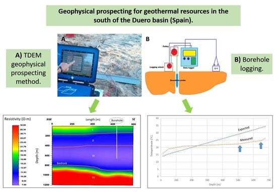
• The time domain electromagnetic (TDEM) method was used to estimate the geological structure of the sedimentary layers even beneath the length of the borehole in study. This method also revealed the depth of the bedrock in the area and how far it was from the end of the borehole logging performed. The geological information obtained with this method could be used to estimate the thermal properties of the ground to assess the performance of future geothermal systems in the location.
• Borehole logging, crossing the entire length of the sounding with a downhole probe, was able to collect data from multiple sensors that provided varied detailed information about the geological composition, traversed aquifers, temperatures throughout the borehole, etc. Additionally, from the detailed information about the geological formations crossed by the logging, it was possible to estimate the thermal properties of the ground to design well fields in geothermal systems with more detail than with the TDEM method.

The results were not completely satisfactory. The thermal gradient from the borehole logging was not as promising as expected. However, in the final part of the borehole, a more pronounced increment of temperature seemed to appear. Perhaps drilling closer to the bedrock (now clearly located by the TDEM method) could find a thermal gradient capable of providing low and medium enthalpy resources that could be used for processes in the food industry, which is a force for economic development in the area.

2. Materials and Methods

2.1. Time Domain Electromagnetic Prospecting Methods

The time domain electromagnetic (TDEM) method of geophysical prospecting was a very important innovation in the field of applied geophysics at the beginning of the 1980s [18,19]. From those years on, the application of the method has allowed for remarkable experiences regarding the capacity of this technique in hydrological science, mining, underground environmental pollution quantification, archeology, etc. In addition, in these years, its advantages over electrical vertical sounding (EVS), limitations, and fields of application have been set. The accumulated experience and the technological improvement in devices have transformed this method into one of the most effective in current geophysics.

Within the TDEM method is time domain electromagnetic sounding (TDEMS), which we performed for this work. TDEMS is a geophysical tool capable of providing very detailed information on the distribution of subsurface resistivity; it can determine its variations both laterally and vertically.

The TDEMS system is classified within the electromagnetic research systems with artificial sources.

Performing a TDEMS consists of injecting a constant current in a loop or transmitter coil (Tx) to generate a constant primary magnetic field. When the current flowing through the Tx is instantaneously interrupted, the primary magnetic field ceases to be constant and decreases its value over time until it becomes zero. In agreement with Faraday’s law, when the ground is exposed to a variable magnetic field in time and a series of electromagnetic inductions of electric currents (Eddy currents) occur in the subsoil (Figure 2). These currents flow in paths closed by the subsoil, laterally migrating in depth and decreasing the current’s intensity over time. This, in turn, generates a decreasing transient secondary magnetic field on the surface.

This secondary field induces a time-varying voltage in the receiving loop (Rx). The voltage drop contains information on the resistivity of the ground because the magnitude and distribution of induced currents depend on the resistivity of the medium.

The electromotive force created in the Rx can be described as follows (Equation (1)) [20]:

$$E=K\ast A\ast N$$

(1)

where E is the electromotive force (V), K is a constant that depends on the magnetic field generated in the Tx (V/m²), A is the area of the Rx (m²), and N is the number of turns in the Tx.

The generated Eddy currents are inducted in the ground and tend to turn away from the generation point at an approximate angle of 30°. The depth of penetration at a given time is given by the following expression (Equation (2)) [20]:

$$Z_d = {\left(\raisebox{1ex}{$2t$}\!\left/ \!\raisebox{-1ex}{$\sigma \mu $}\right.\right)}^{\raisebox{1ex}{$1$}\!\left/ \!\raisebox{-1ex}{$2$}\right.}$$

(2)

where Z_d is the depth of penetration (m), t is the time (s), μ is the permeability (H/m), and σ is the electrical conductivity (S/m).

From Equation (2), it follows that the electrical conductivity of the medium conditions the penetration of the geophysical method. The penetration is directly proportional to the medium resistivity, so the less resistive the medium (marls, clays, etc.), the less the system penetration.

The maximum depth to which we can measure is obtained through Equation (3) [20]:

$$Z_{max} = {\left(\raisebox{1ex}{$2$}\!\left/ \!\raisebox{-1ex}{$25{\pi }^3$}\right.\right)}^{\raisebox{1ex}{$1$}\!\left/ \!\raisebox{-1ex}{$10$}\right.}{\left(\raisebox{1ex}{$│M│$}\!\left/ \!\raisebox{-1ex}{$\sigma V_{noise}$}\right.\right)}^{\raisebox{1ex}{$1$}\!\left/ \!\raisebox{-1ex}{$5$}\right.}$$

(3)

where |M| is the magnetic moment (module) (Am²) and V_noise is the ambient noise (V).

Thus, the maximum depth does depends not only on the moment or conductivity but also on the level of ambient noise [21].

Therefore, the useful depth of research depends on:

• The dimensions of the Tx.
• The intensity of the current flowing through the Tx.
• The duration of the transitory observation time.
• The electrical resistivity of the surface layers and of the ground in general.

The processing of TDEMS (1D) field data is like that of other electrical prospecting methods [22]. Electromotive force, measured as a function of time, becomes the apparent resistivity that is fed an inversion software, which calculates the ground structure with the best possible fit to the curve of the obtained apparent resistivity.

Recently, a system was developed that allows for a 1D dataset to be processed in the form of profiles, thus obtaining an electromagnetic tomography. The software performs joint processing based on specific algorithms (the Spiker algorithm, which adjust the observed apparent resistivities in the best possible way [23]) to obtain 2D sections of the apparent conductivity of the ground. This treatment allows one to correlate the results of the quantitative interpretation of the various TDEMSs (1D) grouped in the same profile, thus obtaining a geo-electric section. The lateral variations of resistivity (lateral resolution) depend on the distance between the loops. More details on the data treatment can be found in Section 3.

2.2. Borehole Logging

The principal aim of geophysical borehole logging techniques is to build a vertical map of the geological composition, some properties of the crossed materials, and the groundwater hydrological conditions of the area.

The determination of which parameter(s) to measure mainly depends on the characteristics of the borehole and the desired information.

Log interpretation mainly includes singular hydro-geophysical units and the sediment layers identified in the descriptive report. Data are collected and stored digitally, and they can be presented at any requested scale.

Table 1. Borehole logging devices, parameters, and purposes.

Log	Parameter Measured	Purpose
Natural gamma	Natural gamma radioactivity	Lithology and the estimation of clay content (40K)
Fluid temperature	Temperature of borehole fluid	Geothermal gradient and water flow
Fluid resistivity	Resistivity of borehole fluid	Water flow and quality
Spontaneous potential (SP)	Electrical potentials between probe and surface electrodes	Lithology, water quality, and, in some cases, fractures in crystalline rock
Single point resistance (SPR)	Resistance of materials between probe and ground surface electrode	Lithology, fracture identification, and location of well screens
Normal resistivity	Apparent resistivity of material	Lithology and water quality

gives a brief description of the magnitudes that were measured in our borehole logging test, as well as their appliances.

2.3. Devices

The TDEMSs were performed by the deployment of 3 square 400 × 400 m loops. The used measuring technique was the one of coincident loops. The repetition of measurements was carried out for each loop to obtain a greater precision in the collection of the field data; this meant that for each one of the three TDEMSs, one register was made by using a staking of 1000 repetitions of the measurement per channel; 73 channels were measured for each one of the registers. However, due to the size of the used loop (400 × 400 m), from channels 35 to 40, the results were heavily affected by the background noise. This was also the case for the first channels, so the first and last channels were discarded in the subsequent processing of the field data.

The equipment used for the TDEMS was the TerraTEM, from the Australian company MONEX GeoScope Geophysical Manufacturing And Consulting Ltd. The TerraTEM incorporates a 10 amp transmitter and a true simultaneous 500 kHz 3-component receiver. Spectral analysis, combined with DSP options, allows the user to monitor and identify local sources of noise; these may be removed using additional filters specific to local site conditions. This device is equipped with a diagnosis menu that provides access to a spectrum analyzer as well as time-domain views of the input signal for the rapid troubleshooting or optimization of acquisition parameters to ambient site conditions.

For the borehole logging, a downhole probe, logging winch, and data logger from Mount Sopris Instruments Company were used. In

Table 2. Downhole probe sensor’s specifications [24].

Sensor	Specifications 1
Natural gamma	Natural gamma sensor composed of a sodium iodide crystal. Gamma range: 0–100,000 cps. Accuracy: 1%. Resolution: 0.02%.
Fluid temperature	Temperature sensor: linear and fast response semi-conductor. Range: −20–80 °C. Accuracy: 1%. Resolution: 0.4 °C.
Spontaneous potential (SP)	Range: −1500–1500 mV (DC). Accuracy: 1%. Resolution: 0.04%.
Single point resistance (SPR)	Range: 0–10,000 Ω. Accuracy: 1%. Resolution: 0.02%.
Resistivity (fluid and normal)	Sensors: stainless steel electrodes. Range: 0–10,000 Ω∙m. Accuracy: 1%. Resolution: 0.02%.

¹ Data from manufacturer (Mount Sopris Instruments, Denver, CO, USA).

, the technical specifications of the sensors included in the downhole probe are detailed.

Figure 3A,B shows the TDEM device during the data acquisition in the location under study and the scheme of the devices for the borehole logging works, respectively.

2.4. Site Description

The area selected for this study is in the north of the province of Ávila (Spain) in the south part of the Duero basin. The southern half of this basin, although not especially renown for this reason, is an area where there are numerous upwellings of groundwater with higher temperatures than could be expected [17]. Figure 4 shows the location and in-situ scheme of the performed TDEM loops.

In

Table 3. Location of the 2D profile endpoints (Figure 3).

Profile Location
	Latitude	Longitude
A	40°55′27.5″ N	4°42′40.3″ W
B	40°55′6.7″ N	4°42′31.2″ W

, the coordinates of the location of the 2D profile from the TDEM method are presented.

As stated in the introduction, this particular location was chosen because the Geological and Mining Institute of Spain [25], where thermal water sources are described for each region, has recorded several promising aquifer formations due to the presence of hot springs in the area.

2.4.1. Geological Description of the Area

The area is characterized by the horizontal or sub horizontal arrangement of materials. Figure 5 shows the geological environment of the location.

Quaternary-age materials are the most common in the location, with some tertiary-age ones appearing mainly on the left side. Concerning the quaternary materials, in general, all the terraces are made up of sand and gravel, with the most recent with predominance being quartz gravels and the old ones mainly being quartzite with a high percentage of quartz in their composition. As for the average grain size, it decreased from the oldest to the most modern levels with sizes of 7–12 and 3–4 cm, respectively.

Tertiary-age materials, which are the oldest of the outcropping rocks in the area, are mainly a set of arkosic sedimentary rocks of beige and whitish color. There are also some cemented sandstones from the lower-middle Miocene [27].

At the specific point where the project was carried out, marked with a blue circle in Figure 4, there are surfaces with or without a deposit of fluvial arkoses with quartz gravel and feldspar, along with the possibility of the appearance of large blocks near the surface.

2.4.2. Hydrogeological Survey

Concerning the hydrogeological indications that were evaluated to choose the location of the study area, information about existing thermal water in the neighborhood was one of the most decisive sources of information. The Geological and Mining Institute of Spain, specifically its Geological Resources Research Department, has been working in the field of mineral and thermal water for decades. The fundamental objective of this service is to contribute to the knowledge and protection of mineral water through research. This labor includes advising administrations, disseminating knowledge about mineral and thermal water to society in general, and promoting and developing the economic sector that uses this water. As such, there is a complete geospatial database that gathers all the information encoded through the years, as well as a large number of documents kept in the archive that are currently digitized and systematized. There is also the Mineral Water Information System (SIAM) for the optimal management of all this information that constitutes a powerful multifunctional tool.

In Figure 6, the hydrogeological map of the area under study is shown; locations A, B, C, D, E, and F are locations with some evidence of thermal water. The Geological and Mining Institute of Spain [28] records the hot springs and classifies them into areas with proven or historical evidence of thermal water and officially declared water.

Figure 6 shows the main sandy aquifer units in the surroundings of our location, which are represented in blue. As can be seen, there are numerous pieces thermal water evidence in the same aquifer of this study, as well as in close ones.

Table 4. Thermal locations from Figure 5 [25].

Location	Description	Current Status
A	20 m deep spring water drilling. Lithology sands, clays, and silts. Water temperature: 14.1 °C.	Officially declared thermal water. Spa in operation.
B	234 m deep spring water drilling. Lithology clays, silts, sands, and gravel. Water temperature: 21.5 °C.	Officially declared thermal water. Spa in operation.
C	Historical evidence.	Dry in surface. Inactive.
D	Historical evidence.	Dry in surface. Inactive.
E	85 m deep spring water drilling. Lithology, clays, and silts. Water temperature: 16.5 °C.	Officially declared thermal water.
F	Evidence.	Officially declared thermal water (in process).

shows a description of each one of these pieces of thermal evidence. In Appendix A, the chemical composition of the thermal water is included (when available).

After gathering all this information on the location of study, the geophysical prospecting work detailed in the previous subsection was carried out.

3. Results

The 2D profile of the ground were obtained with the TDEM method. Figure 7 shows the results. The location of the bore hole where the logging was carried out is also presented.

A, B, C, and D in Figure 6 represent the different layers. A brief explanation of the composition of each one can be seen in

Table 5. Layers from Figure 6.

Layer	Description	Thickness
I	Neogene. Sands and clays.	120–170 m.
II	Neogene. Altered clays with levels of sands and silts.	≈260 m.
III	Neogene. Clays and marl with levels of sands and silts.	350–500 m.
IV	Early Tertiary. Sandstone, shales, and schists.	Bedrock at 800 m (NW) to 900 m (SE).

.

The borehole logging was carried out, and the results of the last 155 m (from 530 to 685 m of depth) are shown in this chapter. The rest of the logging data for the whole well can be found in Appendix B (Figure A1, Figure A2, Figure A3, Figure A4, Figure A5, Figure A6 and Figure A7).

Table 6. Key to the borehole log report.

Column	Measurements
A	Depth (m)
B	Natural Gamma (0–150 counts per second) Spontaneous Potential (300–431 mV) Single point resistance (35–55 Ω)
C	Normal resistivity (0–30 Ω∙m; R8, R16, R32, and R64.)
D	Lithology (graphical description)
E	Lithology (description)
F	Fluid resistivity (214–208 Ω∙m) Temperature (10–30 °C)

shows the key to the different columns in the borehole logging report. Colored text corresponds to the color of the lines on the report.

Figure 8 shows the depth from −530 to −608 of the borehole logging report. Sand layers located at −536 and −550 m, colored in yellow in column D, were reported as most promising for water use of the borehole. These levels should be considered during the casing process of the well.

The black and blue circles in Figure 8 show water inclusions into the borehole from the crossed layers. The black circles point the behavior of the SP (spontaneous potential; mV) reacting to water income with a left leap due to the lower salt content in this water than in the drilling mud. The blue circles indicate the descent in resistivity due to the sand layers with water content. Notice that there is a small depth gap between the sensor’s response in SP and the resistivity, which may have been due to the different locations of the sensors in the downhole probe (which was approximately 2.15 m long).

Figure 9 shows the depth from −609 to −686 of the borehole logging report. It was the end of the logging, so the borehole may have had about 10 m more length. However, for safety reasons, the device stopped data logging at this depth.

The black circles in the SP and the blue circles in the resistivity column mean the same as in Figure 8. Here, there were no sand-only layers, as in the previous section; however, as shown by the logging, there were some layers with sand and water contents entering the borehole. The sudden increase in temperature and fluid resistivity observed at −683 m in Figure 9 should be discarded and can be attributed to pulley braking.

4. Discussion

As shown in Section 3, the temperature results of the borehole logging where not as promising as expected given the thermal evidence in the area. Figure 10 shows a comparison between the expected thermal gradient of the location declared by the IDAE (Diversification and Energy Saving Institute of Spain) [29] and the one measured by the temperature sensor in the downhole probe.

In the measured thermal gradient from the previous figure, two turning points marked with the blue arrows can be observed at around −550 and −650 m of depth. These two sudden increases in temperature seemed to be in line with the contributions of water to the sounding of the layers marked with circles in Figure 8 and Figure 9 found at these depths. Additionally, the approach to the bedrock can explain the fast temperature rising rate as depth increased.

This increase in temperature, if it was caused by the proximity of the bedrock, would indicate that looking for drilling sites closer to its surface would give better results for the thermal gradient. As shown from the TDEM prospecting profile results in Figure 7, the bedrock can be found at −800 m of depth in the north-west side of the area; in comparison, the bedrock can be found at −1000 m of depth in the borehole. Maybe the thermal gradient would be higher there.

Thermal Properties of the Ground by Geophysical Methods

According to previous work, some thermal properties of the ground can be determined by geophysical prospecting methods [22,30,31].

In the previous work “Comparative Analysis of Different Methodologies Used to Estimate the Ground Thermal Conductivity in Low Enthalpy Geothermal Systems” [31], the authors estimated the thermal conductivity of the ground with some geophysical methods (including electrical ones and borehole logging) and then compared the results with the thermal response test (TRT) performed in the same area (the TRT is considered to be the main assay used to obtain the thermal conductivity of the ground [32]).

Following the methods described in the previously mentioned work, the thermal conductivity of the ground was estimated with the data from the TDEM method and the borehole logging. Due to the usual depth of the wells in low-enthalpy geothermal systems of around a maximum of 200 m, this depth was taken into consideration here. In

Table 7. Estimated thermal conductivities from the geophysical methods according to [26].

Geophysical Method	Thermal Conductivity (W/m∙K)	Usual Deviation from TRT
TDEM (NW)	1.48	-
TDEM (SE)	1.37	-
Borehole Logging	1.58	15%

, the obtained results are shown.

Though the usual deviation from the TRT in electrical geophysical methods was established by the authors [33] to be around 14%, in this scenario, the low resolution obtained in the layers near the surface due to the size of the loop in the TDEM method did not allow for a realistic estimation of that deviation.

The TDEM results in Table 7 are divided in two sections because there was horizontal variation in the first 200 m of the 2D profile, as shown in Figure 7.

The effects of the variations in the water table could affect the thermal conductivity value in this kind of geological environment (sedimentary layers) thorough the year. In this case, the borehole logging was performed in summer, so the thermal conductivity in other seasons could be higher due to the ascension of said water table.

5. Conclusions

Through the carried out geophysical works, the geothermal gradient was determined up to a depth of 685 m (the depth of the drilling). The depth of the bedrock and its inclination in the area were also established. Likewise, the most superficial geology data (up to 200 m) were used to establish the conditions of the thermal conductivity of the ground for low-enthalpy geothermal systems in the location.

Temperatures from the borehole logging were not as high as expected, although two promising turning points in the geothermal gradient were found, as can be seen in Figure 10. These turning points seemed to be in line with the water inlets from two sandy layers at around −550 and −650 m of depth.

The position of the bedrock was established (Figure 7) and may be useful in further research in the area. The hypothesis here is that if the borehole was drilled in the NW part of the profile, where the bedrock is not as deep (Figure 7), the temperatures would have been higher. Temperature logging in many different boreholes along the south half of the Duero basin is currently being carried out by our research group, and the results and conclusions will be sources of future publications. The use of TEM apparent resistivity curves for a more precise interpretation of the deep TDEM soundings will also be considered for a future research.

The thermal conductivity of the ground for shallow geothermal systems was also estimated from the data of the borehole logging and the performed TDEM. This was carried out by following methods presented in previous works [33]. By nature, the TDEM method offers much less definition in the most superficial layers, so the expected deviation from a TRT that would have been performed in the area is not included here. However, the expected deviation from a TRT for the more reliable data in shallow layers from the borehole logging is included, again following the work cited above.

References

1. Stefaniuk, M.; Maćkowski, T.; Sowiżdżał, A. Geophysical Methods in the Recognition of Geothermal Resources in Poland—Selected Examples. In Renewable Energy Sources: Engineering, Technology, Innovation; Springer: Cham, Swizerland, 2018; pp. 561–570. [Google Scholar]
2. Pussak, M.; Bauer, K.; Stiller, M.; Bujakowski, W. Improved 3D seismic attribute mapping by CRS stacking instead of NMO stacking: Application to a geothermal reservoir in the Polish Basin. J. Appl. Geophys. 2014, 103, 186–198. [Google Scholar] [CrossRef]
3. Isherwood, W.F.; Mabey, D.R. Evaluation of Baltazor known geothermal resources area, Nevada. Geothermics 1978, 7, 221–229. [Google Scholar] [CrossRef]
4. De Giorgi, L.; Leucci, G. Study of shallow low-enthalpy geothermal resources using integrated geophysical methods. Acta Geophys. 2015, 63, 125–153. [Google Scholar] [CrossRef] [Green Version]
5. Pálmason, G. Geophysical methods in geothermal exploration. In Proceedings of the 2nd UN Symposium on the Development and Use of Geothermal Resources, San Francisco, CA, USA, 20–29 May 1975; Volume 2, pp. 1175–1184. [Google Scholar]
6. Wu, G.; Hu, X.; Huo, G.; Zhou, X. Geophysical exploration for geothermal resources: An application of MT and CSAMT in Jiangxia, Wuhan, China. J. Earth Sci. 2012, 23, 757–767. [Google Scholar] [CrossRef]
7. Montoya, F.G.; Aguilera, M.J.; Manzano-Agugliaro, F. Renewable energy production in Spain: A review. Renew. Sustain. Energy Rev. 2014, 33, 509–531. [Google Scholar] [CrossRef]
8. Banda, E.; Albert-Beltran, J.; Torné, M.; Fernàndez, M. Regional geothermal gradients and lithospheric structure in Spain. In Terrestrial Heat Flow and the Lithosphere Structure; Springer: Berlin/Heidelberg, Germany, 1991; pp. 176–186. [Google Scholar]
9. Piña-Varas, P.; Ledo, J.; Queralt, P.; Marcuello, A.; Bellmunt, F.; Hidalgo, R.; Messeiller, M. 3-D magnetotelluric exploration of Tenerife geothermal system (Canary Islands, Spain). Surv. Geophys. 2014, 35, 1045–1064. [Google Scholar] [CrossRef]
10. Navarro, J.Á.S.; López, P.C.; Perez-Garcia, A. Evaluation of geothermal flow at the springs in Aragon (Spain), and its relation to geologic structure. Hydrogeol. J. 2004, 12, 601–609. [Google Scholar] [CrossRef]
11. EU. DIRECTIVE (EU) 2018/2001 OF THE EUROPEAN PARLIAMENT AND OF THE COUNCIL of 11 December 2018 on the Promotion of the Use of Energy from Renewable Sources. Off. J. Eur. Union 2018, 5, 82–209. [Google Scholar]
12. Sáez Blázquez, C.; Farfán Martín, A.; Nieto, I.M.; González-Aguilera, D. Economic and environmental analysis of different district heating systems aided by geothermal energy. Energies 2018, 11, 1265. [Google Scholar] [CrossRef] [Green Version]
13. Harvey, C.C.; Harvey, M.C. The prospectivity of hotspot volcanic islands for geothermal exploration. In Proceedings of the World Geothermal Congress 2010, Bali, Indonesia, 25–30 April 2010. [Google Scholar]
14. Colmenar-Santos, A.; Folch-Calvo, M.; Rosales-Asensio, E.; Borge-Diez, D. The geothermal potential in Spain. Renew. Sustain. Energy Rev. 2016, 56, 865–886. [Google Scholar] [CrossRef]
15. Chamorro, C.R.; García-Cuesta, J.L.; Mondéjar, M.E.; Linares, M.M. An estimation of the enhanced geothermal systems potential for the Iberian Peninsula. Renew. Energy 2014, 66, 1–14. [Google Scholar] [CrossRef]
16. Schellschmidt, R.; Hurter, S.; Förster, A.; Huenges, E. Atlas of Geothermal Resources in Europe; Office for Official Publications of the European Communities: Brussels, Belgium, 2002. [Google Scholar]
17. Mapa Hidrogeológico de España a escala 1:100.000. (Hojas 36, 37 y 38); IGME, Instituto Geológico y Minero de España: Madrid, Spain. Available online: https://info.igme.es/cartografiadigital/geologica/mapa.aspx?parent=../tematica/tematicossingulares.aspx&Id=19 (accessed on 1 July 2020).
18. Harthill, N. Time-domain electromagnetic sounding. IEEE Trans. Geosci. Electron. 1976, 14, 256–260. [Google Scholar] [CrossRef]
19. Rodriguez, J.C.; JC, R. Inversion of TDEM (near-zone) sounding curves with catalog interpolation. Pascal Francis 1978, 73, 57–69. [Google Scholar]
20. Nabighian, M.N.; Macnae, J.C. Time domain electromagnetic prospecting methods. Electromagn. Methods Appl. Geophys. 1991, 2 Part A, 427–509. [Google Scholar]
21. Munkholm, M.S.; Sørensen, K.I.; Jacobsen, B.H. Characterization and in-field suppression of noise in hydrogeophysics. In Symposium on the Application of Geophysics to Engineering and Environmental Problems; Society of Exploration Geophysicists: Tulsa, OK, USA, 1995; pp. 339–347. [Google Scholar]
22. Nieto, I.M.; Martín, A.F.; Blázquez, C.S.; Aguilera, D.G.; García, P.C.; Vasco, E.F.; García, J.C. Use of 3D electrical resistivity tomography to improve the design of low enthalpy geothermal systems. Geothermics 2019, 79, 1–13. [Google Scholar] [CrossRef]
23. Law, D.; Noh, K.A.M.; Rafek, A.G.M. Application of Transient Electromagnetic (TEM) Method for Delineation of Mineralized Fracture Zones. In IOP Conference Series: Earth and Environmental Science; IOP Publishing: Bristol, UK, 2019; Volume 279, p. 012038. [Google Scholar]
24. Mount Sopris Instruments, Denver, CO, USA. Available online: https://mountsopris.com/ (accessed on 1 July 2020).
25. Baeza Rodríguez-Caro, J.; López Geta, J.A.; Ramírez Ortega, A. Aguas Minerales y Termales de España; IGME, Instituto Geológico y Minero de España: Madrid, Spain; Chapter 6.1, ISBN: 84-7840-424-4. Available online: https://aguasmineralesytermales.igme.es/inventario-aguas-minerales-termales (accessed on 1 July 2020).
26. MAGNA 50, MAPA GEOLÓGICO DE ESPAÑA 1:50.000, HOJA 481, Nava de Arévalo; IGME, Instituto Geológico y Minero de España: Madrid, Spain, 2003.
27. Carreras, F.; Molina, E. Memoria de la Hoja N° 481 (Nava de Arévalo). In Mapa geológico de España E 1:50.000 (MAGNA); Segunda Serie, Primera Edición; IGME: Madrid, Spain, 1982; Depósito Legal M-29894-1982; ISSN 0373-2096. [Google Scholar]
28. Aguas Minerales y Termales de España; IGME, Instituto Geológico y Minero de España: Madrid, Spain; Mapa Hidrogeológico de España a escala 1:100.000. (Hoja 37). Available online: https://info.igme.es/cartografiadigital/geologica/mapa.aspx?parent=../tematica/tematicossingulares.aspx&Id=19 (accessed on 1 July 2020).
29. Ministerio de Industria. Energía y Turismo, IDAE (Instituto Para la Diversificación y Ahorro de la Energía), Manual de Geotermia; Ministerio de Industria: Madrid, Spain, 2008. [Google Scholar]
30. Sáez Blázquez, C.; Carrasco García, P.; Nieto, I.M.; Maté-González, M.Á.; Martín, A.F.; González-Aguilera, D. Characterizing Geological Heterogeneities for Geothermal Purposes through Combined Geophysical Prospecting Methods. Remote Sens. 2020, 12, 1948. [Google Scholar] [CrossRef]
31. Blázquez, C.S.; Martín, A.F.; García, P.C.; González-Aguilera, D. Thermal conductivity characterization of three geological formations by the implementation of geophysical methods. Geothermics 2018, 72, 101–111. [Google Scholar] [CrossRef]
32. Sanner, B.; Hellström, G.; Spitler, J.; Gehlin, S. Thermal response test–current status and world-wide application. In Proceedings of the World Geothermal Congress, Antalya, Turkey, 24–29 April 2005; International Geothermal Association: Bochum, Germany, 2005; Volume 1436, p. 2005. [Google Scholar]
33. Sáez Blázquez, C.; Martín Nieto, I.; Farfán Martín, A.; González-Aguilera, D.; Carrasco García, P. Comparative Analysis of Different Methodologies Used to Estimate the Ground Thermal Conductivity in Low Enthalpy Geothermal Systems. Energies 2019, 12, 1672. [Google Scholar] [CrossRef] [Green Version]
Figure 1. Types of geothermal resources (* EGS stands for enhanced geothermal systems and HDR stands for hot dry rock).
Energies 13 05397 g001
Figure 2. Eddy currents to the underground.
Energies 13 05397 g002
Figure 3. (A) TerraTEM time domain electromagnetic (TDEM) device during the data acquisition phase of this study. (B) Borehole logging equipment (scheme).
Energies 13 05397 g003
Figure 4. Location and site of prospecting data.
Energies 13 05397 g004
Figure 5. Geological survey of the study area [26].
Energies 13 05397 g005
Figure 6. Hydrogeological map of the area [28].
Energies 13 05397 g006
Figure 7. 2D profile gathered from the TDEM method.
Energies 13 05397 g007
Figure 8. Borehole logging report (from −531 to −608 m).
Energies 13 05397 g008
Figure 9. Borehole logging report (from −609 to −685 m). End of the borehole logging.
Energies 13 05397 g009
Figure 10. Expected vs. measured temperatures across the borehole.
Energies 13 05397 g010