Article

Analysis of Random Forest Modeling Strategies for Multi-Step Wind Speed Forecasting

by
Daniel Vassallo
1,*,
Raghavendra Krishnamurthy
2,
Thomas Sherman
3 and
Harindra J. S. Fernando
1
1
Department of Civil & Environmental Engineering and Earth Sciences (CEEES), University of Notre Dame, Notre Dame, IN 46556, USA
2
Pacific Northwest National Laboratory, Richland, WA 99354, USA
3
CRCL Solutions, LLC, South Bend, IN 46617, UAS
*
Author to whom correspondence should be addressed.
Energies 2020, 13(20), 5488; https://doi.org/10.3390/en13205488
Submission received: 19 September 2020 / Revised: 12 October 2020 / Accepted: 14 October 2020 / Published: 20 October 2020
(This article belongs to the Special Issue Recent Advances in Wind Power Meteorology)

Abstract

:
Although the random forest (RF) model is a powerful machine learning tool that has been utilized in many wind speed/power forecasting studies, there has been no consensus on optimal RF modeling strategies. This study investigates three basic questions which aim to assist in the discernment and quantification of the effects of individual model properties, namely: (1) using a standalone RF model versus using RF as a correction mechanism for the persistence approach, (2) utilizing a recursive versus direct multi-step forecasting strategy, and (3) training data availability on model forecasting accuracy from one to six hours ahead. These questions are investigated utilizing data from the FINO1 offshore platform and Atmospheric Radiation Measurement (ARM) Southern Great Plains (SGP) C1 site, and testing results are compared to the persistence method. At FINO1, due to the presence of multiple wind farms and high inter-annual variability, RF is more effective as an error-correction mechanism for the persistence approach. The direct forecasting strategy is seen to slightly outperform the recursive strategy, specifically for forecasts three or more steps ahead. Finally, increased data availability (up to ∼8 equivalent years of hourly training data) appears to continually improve forecasting accuracy, although changing environmental flow patterns have the potential to negate such improvement. We hope that the findings of this study will assist future researchers and industry professionals to construct accurate, reliable RF models for wind speed forecasting.

Graphical Abstract

1. Introduction

Machine learning (ML) methods are becoming increasingly popular within the wind energy sector, especially for wind speed/power forecasting [1]. Increased usage of ML, and statistical modeling in general, for forecasting purposes is due to a timescale gap in the utility of other conventional techniques. Numerical weather prediction (NWP) models struggle to predict highly variable small-scale atmospheric characteristics (e.g., surface wind speeds) and are typically limited to forecasts of six or more hours ahead due to high computational costs [2]. Conversely, the naive persistence approach (i.e., U τ + n = U τ ; U is mean streamwise wind speed, τ a given time step, and n the number of timesteps in advance to be forecasted) is most useful for very short-term (<30 min) forecasts, as its accuracy decreases with increasing forecasting timescale. Statistical and ML approaches have therefore become increasingly common for short-term forecasting (30 min to 6 h ahead) because of their effectiveness, inexpensiveness, and modeling ease [3].
Random forest (RF) is a ML modeling methodology that has shown great promise for wind forecasting purposes. Lahouar and Slama [4] forecasted hour-ahead wind power using up to 18 input variables, showing that RF modeling is robust to noisy or irrelevant inputs. Feng et al. [5] used RF as a constituent within an ensemble modeling framework with deep feature selection, improving hourly wind power forecasting accuracy by up to 30% over a single-algorithm model. Niu et al. [6] utilized a hybrid wavelet decomposition weighted RF model which had been optimized by the niche immune lion algorithm to forecast ultra-short-term wind power. The developed model outperformed a typical RF model, a neural network, and a support vector machine. Sun et al. [7] used a hybrid model combining a deep belief network (to forecast wind speed) and an optimized RF to forecast wind power. Shi et al. [8] created an improved RF model which utilized 2-stage feature selection and decision tree reorganization to forecast 15-minute wind power, showing that the improved model outperforms the original RF, a neural network, and a support vector machine. Lastly, Vassallo et al. [9] tested the utility of a multitude of atmospheric input features used within an RF model for wind speed forecasting.
The above studies provide valuable insights into how the RF model may be utilized in an attempt to create an optimal ML architecture for wind forecasting. This study deviates from many of those above in that, rather than creating a single optimal RF architecture, it asks fundamental questions about best modeling practices when using the RF model for wind speed forecasting. In the authors’ opinion, at least three questions are particularly pressing for ML wind speed forecasting in the wind energy industry and will therefore be investigated in this study:
  • Does RF provide better results as a standalone model or as an error-correction mechanism for a naive model?
  • What is the effect of making a multi-step prediction based on a recursive (step-by-step) vs. a direct (single jump) methodology?
  • How much training data is required for model performance to show asymptotic behavior (i.e., reach a stable optimum even as more training data is added)?
To the authors’ knowledge, no definitive conclusions have been made for any of these three questions. The first question, as posed, is an attempt to discover whether a hybrid model will outperform a standalone model. While hybrid and ensemble methodologies (which are typically far more complex) have been shown to outperform their individual modeling components [10], the proposed hybrid model is unique in that it is highly interpretable and requires the same amount of computational power as the standalone RF model. Crucially, the only difference between the standalone RF model and the hybrid model is the choice of target variable (described further in Section 2.3).
The second question has been addressed by Wang et al. [11] and Ahmed and Khalid [12], with varying results. Wang et al. [11], in an analysis of 48 different hybrid models tested on data from four wind farm sites, found nearly negligible differences between the recursive and direct strategies. Ahmed and Khalid [12], however, found that the direct strategy conclusively outperformed the recursive strategy when used for hourly forecasts two to six hours ahead. We hope to add to these conclusions by investigating the efficacy of both modeling strategies at two climatologically and topographically disparate sites.
The third question is an investigation into the extent of model improvement with increasing data availability. Of particular interest is whether model accuracy shows asymptotic behavior and reaches a stable optimum when given almost a decade of training data. This final investigation can help both researchers and industry professionals understand how much RF forecasting models should be expected to improve if the data collection period is extended.
In this study, we investigate these questions in two separate climatological regions using a RF model to forecast hourly wind speeds one to six hours ahead. The model itself is deliberately kept as simple as possible to best quantify the effects of each modeling strategy and variation. Data is taken from the FINO1 platform in the North Sea and the Atmospheric Radiation Measurement (ARM) Southern Great Plains (SGP) central facility site (hereafter referred to as SGP C1) near Lamont, Oklahoma. Testing proceeds in two stages, with the first two questions investigated concurrently and the third question investigated separately. It must be stated that the quantitative findings of this investigation are not expected to be representative of every dataset or location. However, the findings are expected to be an instructive, reliable reference for future studies and industry practices.
Section 2 gives an overview of the RF model and testing methodology as well as a description of the testing sites and data processing performed to ensure accurate modeling results. Section 3 provides testing results and discussion for both the FINO1 and SGP C1 sites. Finally, conclusions are given in Section 4.

2. Materials and Methods

2.1. Random Forest Regression

RF regression [13] is an ensemble ML model that relies on the aggregation of weak predictors, namely regression trees [14], to provide an accurate and reliable prediction. Each of the trees is constructed independently using a subset of the training data, a process called bootstrap aggregation or bagging. Each tree samples randomly with replacement from the training data, made up of an input set (made up of multiple input features) X = x 1 , x 2 , ... , x N and a target set Y = y 1 , y 2 , . . . , y N where N is the number of samples. Each tree f m is then fit to its unique subset of the training data. Once all trees have been constructed, predictions ( y ^ ) are made (on the testing set) by averaging the individual regression tree outputs, i.e., y ^ = 1 M m = 1 M f m ( x ) where M is the total number of regression trees and x is a sample in the testing set.
Splits in a regression tree are determined via impurity reduction, scilicet, the reduction of the prediction’s mean squared error (MSE). General regression tree aggregation algorithms allow each tree to choose the best of all input features with which to make every split. RF, however, only allows each split to be made from a subset of the entire feature set, allowing for a more diverse and uncorrelated set of weak predictors.
This investigation utilizes a forest of 1000 trees for each test. The sci-kit learn Python library was used for model construction [15]. To ensure prediction stability, each test is performed 10 times and the average over these runs is reported. Providing each tree with 50% of the input features for each split was empirically determined to provide optimal results. Additionally, although the RF algorithm is already fortified against overfitting [13,16], a minimum of 100 samples is required to make each split. This regularization technique boosts the algorithm’s generalizability, ideally resulting in a model which provides accurate predictions for peripheral future samples.

2.2. Testing Sites

FINO1 is an offshore measurement platform in the North Sea. The platform is located approximately 45 km north of Borkum, Germany and has multiple operational wind farms (the first of which was constructed in 2009) in its immediate vicinity. FINO1, which has been operational since 2004, extends to a height of 100 m above mean sea level (MSL) and has a variety of sensors (generally) at 10 m vertical intervals along the mast (visualization of wind speed sensors may be seen in Figure 1 of [17]). The utilized measurements come from a cup anemometer, wind vane, and temperature sensor 70 m MSL. The 70 m cup anemometer measurements have 2% uncertainty [18], but for this study all data are assumed to be true. Data were recorded in 10-min increments. To attain hourly measurements, six 10-min periods are averaged. A number of measurements are corrupted, and therefore a minimum of 50% of the time periods (three of the six 10-min measurements) in the hourly time frame are required for an acceptable hourly measurement. All time periods that do not satisfy this requirement are removed. A violin plot of annual wind speed distributions at the FINO1 site can be seen in Figure 1a. No data was available in 2008, 2009, 2013, or 2014.
SGP C1 is a heavily instrumented field measurement site operated by the US Department of Energy, with a variety of in situ and remote-sensing instruments in northern Oklahoma. The SGP observatory was established in 1992 to support the improvement of global circulation modeling [19]. The instrumentation utilized is a temperature, humidity, wind, and pressure sensors (THWAPS) system that was operational from September 1999–January 2016 [20]. The wind speed measurements have ±1% wind speed uncertainty [21], but as with FINO1 all measurements are assumed true. Data from 2003–2014 are used in this study. The SGP C1 site is located in relatively flat and rural terrain. In 2012, a wind farm was constructed to the southwest of SGP C1 (nearest turbine at least 60 rotor diameters away). Owing to the staggered orientation of the wind farm, predominantly low frequency of southerly wind direction at the SGP site, and the distance from SGP C1 to the nearest turbines, wind measurements at SGP C1 are not expected to be impacted from the wind farm built in 2012. Standard quality control procedures provided by the instrument mentors are used to remove questionable data. Data were recorded in 30-min increments and availability of both half-hour measurements is required for the creation of an acceptable hourly measurement. All time periods that do not satisfy this requirement are removed. Annual wind speed distributions at the SGP C1 site can be seen in Figure 1b.

2.3. Data Preprocessing

The previously described data averaging leads to the creation of a robust dataset for the RF model. The utilized sensor data includes mean and standard deviation of streamwise wind speed (U and σ u , respectively), wind direction θ , and temperature T. U and σ u are utilized to obtain turbulence intensity measurements ( T I = σ u U ). Time of day t and day of year d were also used as input information. θ , t and d are split into two oscillating components (e.g., t 1 and t 2 , both ranging from −1 to 1) to remove any potential discontinuities in the data. Pertinent meteorological statistics at both FINO1 and SGP C1 can be seen in Table 1.
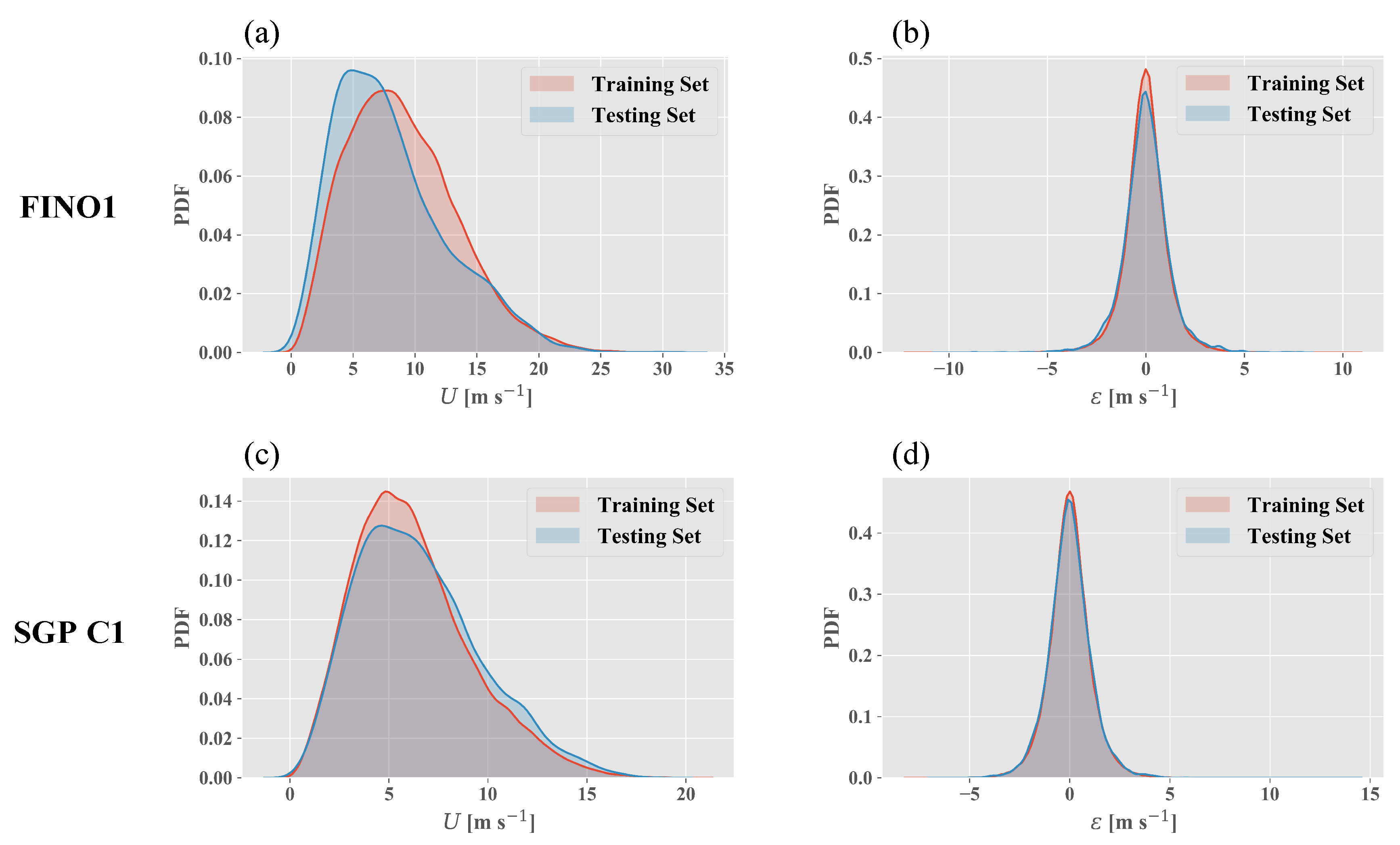
As was mentioned in Section 1, the difference between the standalone RF model and the hybrid persistence–RF model is simply the choice of target variable. The standalone RF model predicts the absolute wind speed at the time period of interest (i.e., target variable y = U τ + n ). When used to correct the persistence error ( ε ), the RF model predicts the difference between the wind speed at the current time period and that at the time period of interest (i.e., y = ε = U τ + n U τ ). This is otherwise known as differencing, a technique commonly used in statistical forecasting to remove trends in the data, thereby ensuring constant long-term statistical properties [22,23,24] (a more detailed explanation of statistical stationarity and differencing can be found in Hyndman and Athanasopoulos [24]). The effects of differencing can be seen in Figure 2, where the target variable training and testing probability distribution functions (PDFs) for the standalone (Figure 2a,c) and hybrid (Figure 2b,d) models are shown. The differencing proposed in this investigation is different from that used in many statistical models in that we only difference the target variable (all inputs are unaltered). The RF error prediction is then added to the persistence prediction to get a final wind speed forecast.
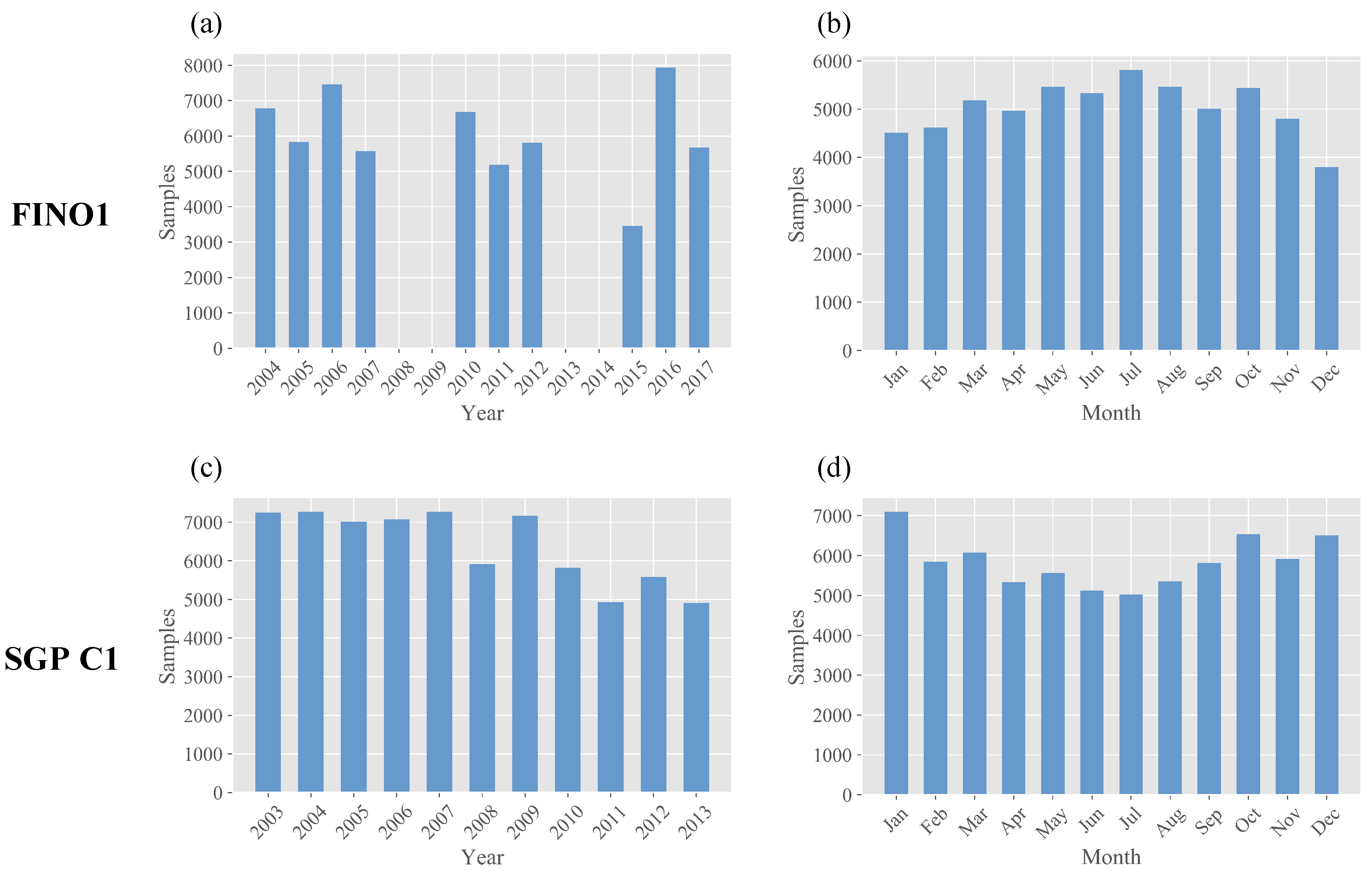
Data was split chronologically into a training and testing set. The first 90% of the data, over 57,000 samples (January 2004–August 2017 for FINO1; January 2003–November 2013 for SGP C1), was used for training. The final 10% of data, more than 6000 samples (August 2017–August 2018 for FINO1; November 2013–December 2014 for SGP C1), was used for testing. More details about data samples, including annual and monthly training data availability, can be found in Appendix A.

2.4. Testing

Tests investigate hourly forecasts from one to six hours ahead. Testing is performed in two stages. The first stage examines the first two questions stated in Section 1, i.e., RF as a standalone model vs. error correction mechanism, and making recursive vs. direct multi-step forecasts. This requires the creation and testing of four model-target combinations (hereafter referred to as modeling strategies) for each forecasting timescale. The modeling strategy with the highest forecasting accuracy is then used for the second stage of testing, which investigates the model’s improvement with increasing training data availability.
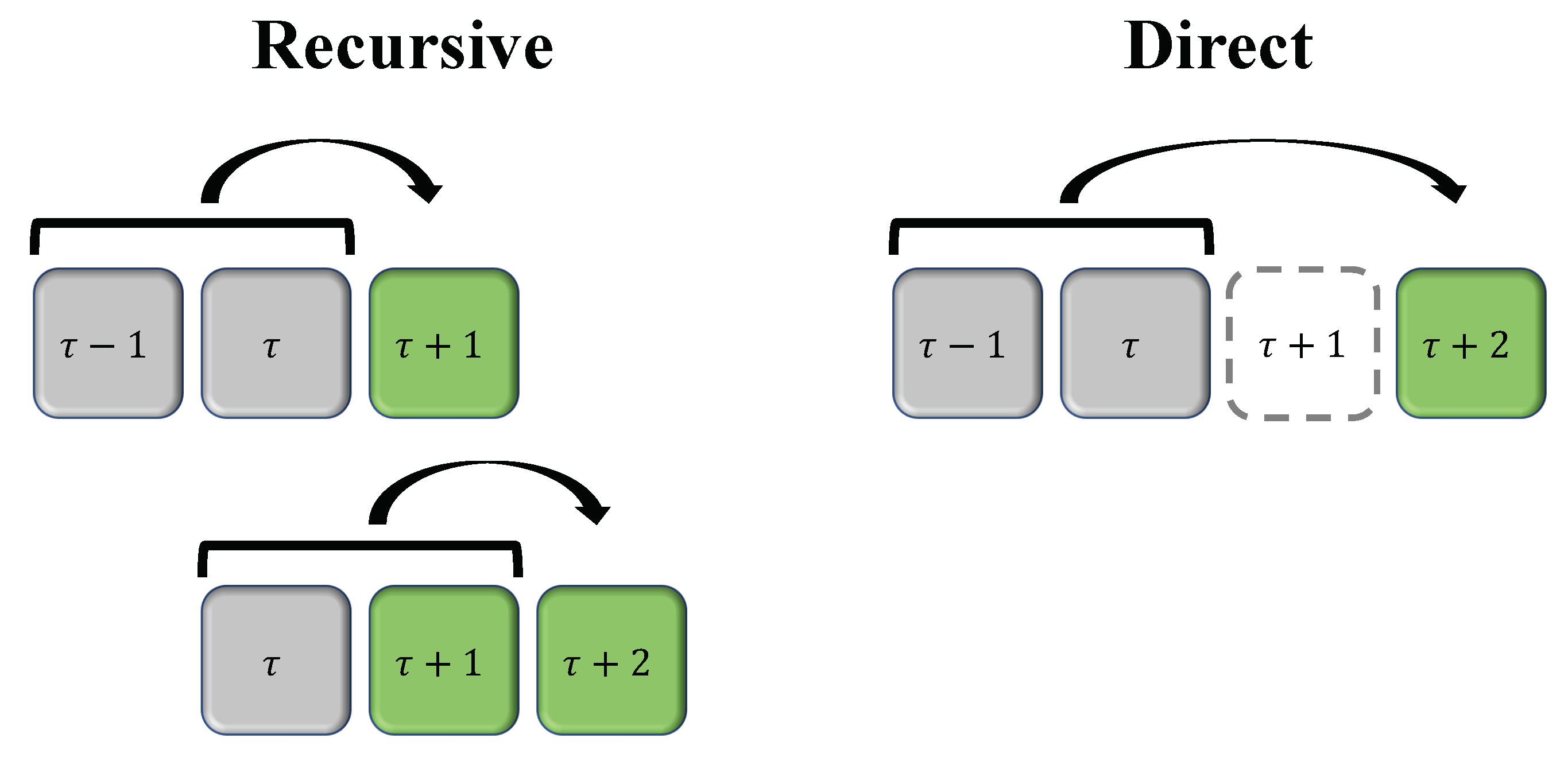
For the first stage, four modeling strategies are investigated: recursive standalone RF models (RS), recursive RF models predicting persistence modeling error (RE), direct standalone RF models (DS), and direct RF models predicting persistence modeling error (DE). Recursive modeling requires that, for multi-step predictions, all non-temporal input variables be forecast for every time step (e.g., the 6-h RS model requires prediction of U, T I , θ , and T from one to six hours in advance). In contrast, direct models skip all timesteps prior to the forecasting timestep of interest (e.g., the 6-h DS model directly predicts U six hours ahead exclusively utilizing known information from the current and past timesteps). An illustration of both model types can be seen in Figure 3, and a detailed explanation of both strategies can be found in Bontempi et al. [25]. A series of 480 testing runs are performed for the first stage of testing, as there are four modeling strategies (RS, RE, DS, DE) each forecasting six distinct timesteps in the future at two sites, with 10 runs per test to ensure prediction stability.
The second stage of testing takes the best modeling strategy (as quantified by root mean squared error, as described below) and determines how the amount of training data affects forecasting accuracy. The full training sets at both sites consist of over 6.5 equivalent years of data (8760 hourly samples per equivalent year). Therefore, to test the strategy’s performance, the model is given only a single equivalent year of training data and forecasting accuracy is calculated. This process continues in annual increments, with the model given 2→6 equivalent years of data to train on. Thus, 720 testing runs are performed (one modeling strategy, six timesteps, six quantities of training data, two sites, 10 runs per test for stability), allowing for an in-depth analysis of how the modeling strategy improves with data availability.
Root mean squared error (RMSE; Equation (1) where U ^ i is the predicted wind speed, U i is the true target wind speed, and N again is the number of samples) is the metric utilized to determine forecasting accuracy. The models’ RMSE values are compared to those of the persistence model and the percent improvement is calculated to ensure the models perform better than a naive predictor.
R M S E = 1 N i = 1 N ( U ^ i U i ) 2
All tests require nine total input features (six distinct input features, three of which have two oscillatory components): U, T I , T, θ (two components), t (two components), and d (two components). Vassallo et al. [9] recently showed that U, T I , T, t, and θ are the most important atmospheric inputs for hourly wind speed forecasting (d excluded from the study due to a lack of data availability). As is shown in Figure 3, each of these input features are taken from the previous two time periods ( τ 1 and τ ) and utilized for the prediction. The accuracy of the hybrid error correction model is determined by adding U τ to the prediction, giving a final absolute prediction of U ^ τ + n ( U ^ τ + n = U τ + ε ^ ; ε ^ is the predicted persistence model error). Each test is performed 10 times, and the average value of these tests is reported. The standard deviation of the prediction for all tests is below 0.003 m s 1 , confirming model stability and validating testing results.

3. Results and Discussion

3.1. FINO1

3.1.1. Modeling Strategy Comparison

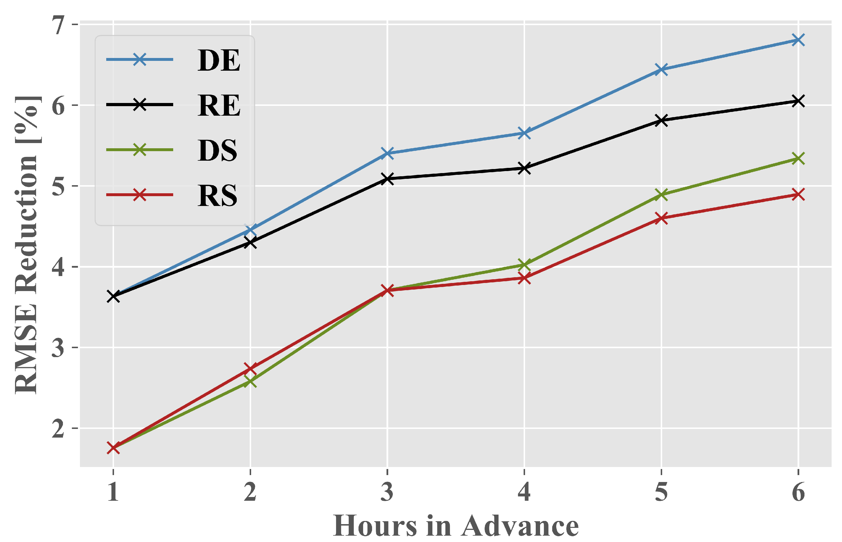
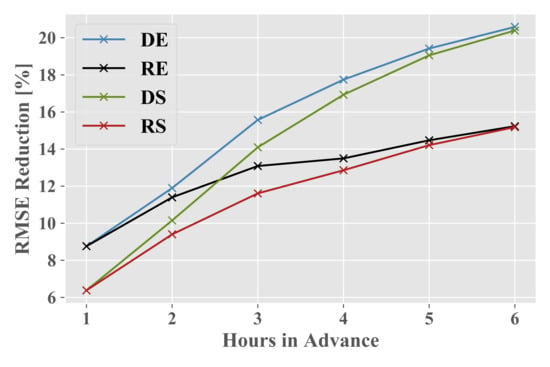
As Figure 4 shows, DE outperforms all other modeling strategies for all multi-step forecasts at the FINO1 testing site, providing up to ∼7% improvement over the persistence model for a 6-h forecast. Standalone RF models are outperformed by their hybrid counterparts, while direct forecasts show slight improvement over their recursive counterparts. FINO1 testing metrics for all four modeling strategies, as well as that obtained by the persistence model, can be seen at the top of Table A2 in Appendix B.
The results show that, at the FINO1 site, hybrid persistence–RF models tend to outperform the standalone RF models. This is not surprising, as certain statistical models require the removal of trends to enforce a constant mean and standard deviation for a given time series, allowing the model to obtain optimal results [24]. While wind speeds tend to have a relatively stable multi-year mean and variance, the effects of inter-annual variability (IAV) may skew any single year’s wind speed distribution. IAV is typically calculated as I A V = 100 σ U ¯ U ¯ where U ¯ is the mean of a representative period’s annual wind speeds and σ U ¯ the standard deviation of annual wind speeds over the entire representative period, thus making IAV a percentage of the period’s overall mean annual wind speed [26]. IAV values of 6% are used as a representative estimate within the wind energy industry [27]. Therefore, the 8.0% IAV observed at the FINO1 site is a clear indicator that the wind speeds observed over any given year can be considerably skewed when compared to the period’s overall average (Figure 1a). The results of such a phenomenon can be seen in Figure 2a,b. From this figure it is clear that the testing dataset has a much smaller mean hourly U (8.07 m s 1 ) than that of the training dataset (8.99 m s 1 ). However, the distributions of training and testing ε remain relatively similar. One of the primary assumptions of ML model efficacy and suitability is that the target variable distribution remains constant between the training and testing sets [28]. These results suggest that the distribution of ε is less affected by IAV, thereby making it a more suitable target variable for ML forecasting.
Whereas models predicting ε clearly outperform those predicting U, the effect of making direct vs. recursive forecasts is much more subtle, corroborating the findings of Wang et al. [11]. The direct and recursive models provide the exact same improvement for single-step forecasting because, for this case, they are identical models. Both strategies perform similarly for forecasts up to three hours in advance, indicating that there may be general limitations to the amount of improvement that may be seen by such a forecasting model given limited atmospheric information at a single location. The direct model outperforms the recursive model for forecasts more than three hours ahead, particularly when the differencing strategy is utilized. This suggests that, at the FINO1 site, it is likely more beneficial to utilize direct forecasting. However, it is far more important to set ε as the target variable in order to minimize the effects of IAV.
Figure 5a,b shows the reduction in RMSE obtained by the DE model at FINO1 (across all forecasting timescales) partitioned by month and hour of the day, respectively. The DE model performs poorly in late winter and early spring, performing ∼3.5% worse (on average) than the persistence model during the months of February and March. These two months primarily experience cold southeasterly flow at FINO1, with flow from the German coast experiencing wake effects prior to reaching the measurement location [29]. However, the DE model outperforms the persistence model for all other months, showing an RMSE reduction of almost 10% in both April and December. There is a clear seasonal pattern to the predictive improvement, as the DE model consistently provides a considerable RMSE reduction in the summer and early winter.
Model improvement shows a diurnal as well as a seasonal trend (Figure 5b). The DE model shows minimal improvement during the morning hours (local time = UTC + 0100 h), but considerably improves upon the persistence model in the afternoon and early evening. The model’s greatest (average) improvement comes at 1700 UTC, as RMSE is reduced by 15% for forecasts four or more hours ahead. The persistence model’s RMSE is highest during the afternoon and early evening (not shown). The DE model is able to drastically improve upon the persistence model during these hours, likely accounting for the evening transition from a daytime convective regime to a stable nocturnal regime.
Monthly and hourly RMSE reduction (and occasional inflation) are driven by local atmospheric conditions. Wind farms surround the offshore measurement site, generating wakes which lead to wind speed deficits and may impact the predictive capability of ML models. Poor performance may also derive from the high variability in atmospheric stability at FINO1, e.g., wind ramps (rapid increases or decreases in wind speed) resulting from cooler air masses that travel southwards and cause atmospheric instability. Since the simple RF model used in this analysis does not contain any information on surrounding meteorological conditions or atmospheric stability (such as Richardson number, air and sea temperature difference, etc.), the RF model is unable to clearly distinguish or characterize such effects. A RF model given atmospheric stability input features could likely better interpret some of the hourly and monthly variability observed in this analysis [9].

3.1.2. Training Data Availability

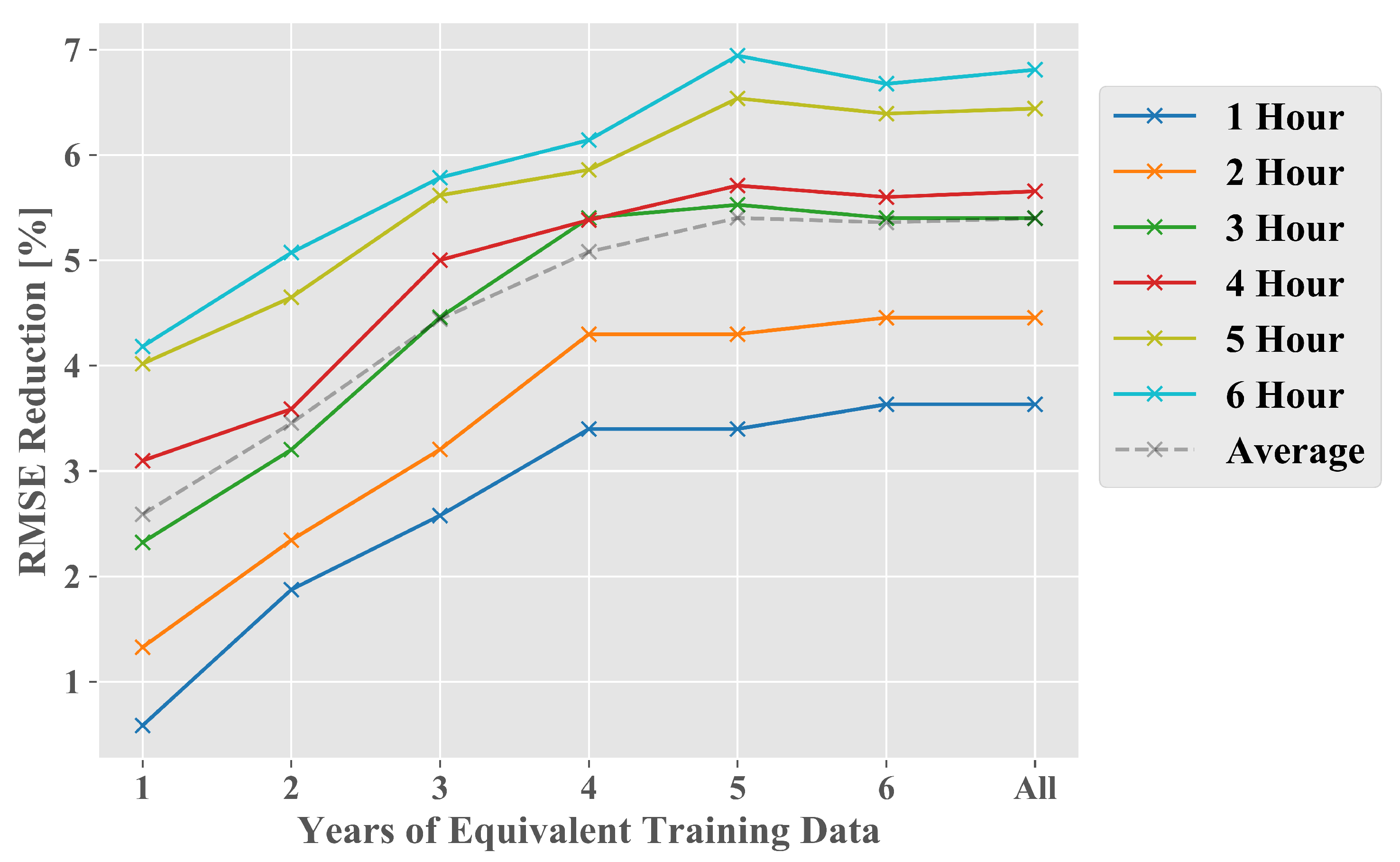
Figure 6 shows the improvement obtained by the DE strategy compared to persistence at FINO1, for forecasts one to six hours ahead, when given between one equivalent year of training data (8760 samples) and the full training dataset (approximately seven equivalent years of data). Forecasting accuracy clearly improves with increasing data availability, particularly when less than four equivalent years of training data is available. However, there are diminishing returns above four equivalent years of availability, particularly for predictions less than four hours ahead. Improvements completely stall when the model is given more than five equivalent years of data, with the RF error correction, on average, decreasing RMSE by more than 5%. Testing metrics may be found in Table A3 in Appendix B.
The slow and steady improvement of the DE strategy with increasing data availability (up to 4–5 equivalent years) is interesting in that it seems to give a clear cut-off for the amount of data that is necessary to achieve optimal forecasting results at the FINO1 site. According to the findings, the model’s forecasting capability will only improve with up to five years of training data. Above this limit, the model does not seem to improve. This is almost certainly due to the construction of wind farms in the surrounding region beginning in 2009. The wakes from such farms alter the surrounding flow field [30], thereby negating the utility of data collected prior to wind farm construction. The first wind turbine from the Alpha Ventus wind farm came online in August of 2009, or about a fifth of the way through the fifth equivalent year of FINO1 training data (corresponding to ∼4.2 equivalent years of training data). These wind farms appear to impact the overall wind climatology at the FINO1 site, as average annual wind speeds from 2016–2018 are lower than those prior to 2010 (Figure 1a). Utilizing training data collected during a previous flow regime (unimpeded flow) to predict the current flow regime (large turbine wake effects) is a potentially deleterious practice as much of the training and testing data originate from disparate atmospheric processes (i.e., the training and testing data have different properties and distributions). However, prediction accuracy does not considerably decrease when free-flow data (before 2010) is included in the training set. Upstream information in the free-flow regime is likely still relevant to the obstructed flow regime, although less so than information recorded after wind farm construction. Regardless, the newly constructed wind farms clearly have a nugatory effect on the algorithm’s pattern recognition abilities, causing a stagnation in prediction accuracy.

3.2. SGP C1

3.2.1. Modeling Strategy Comparison

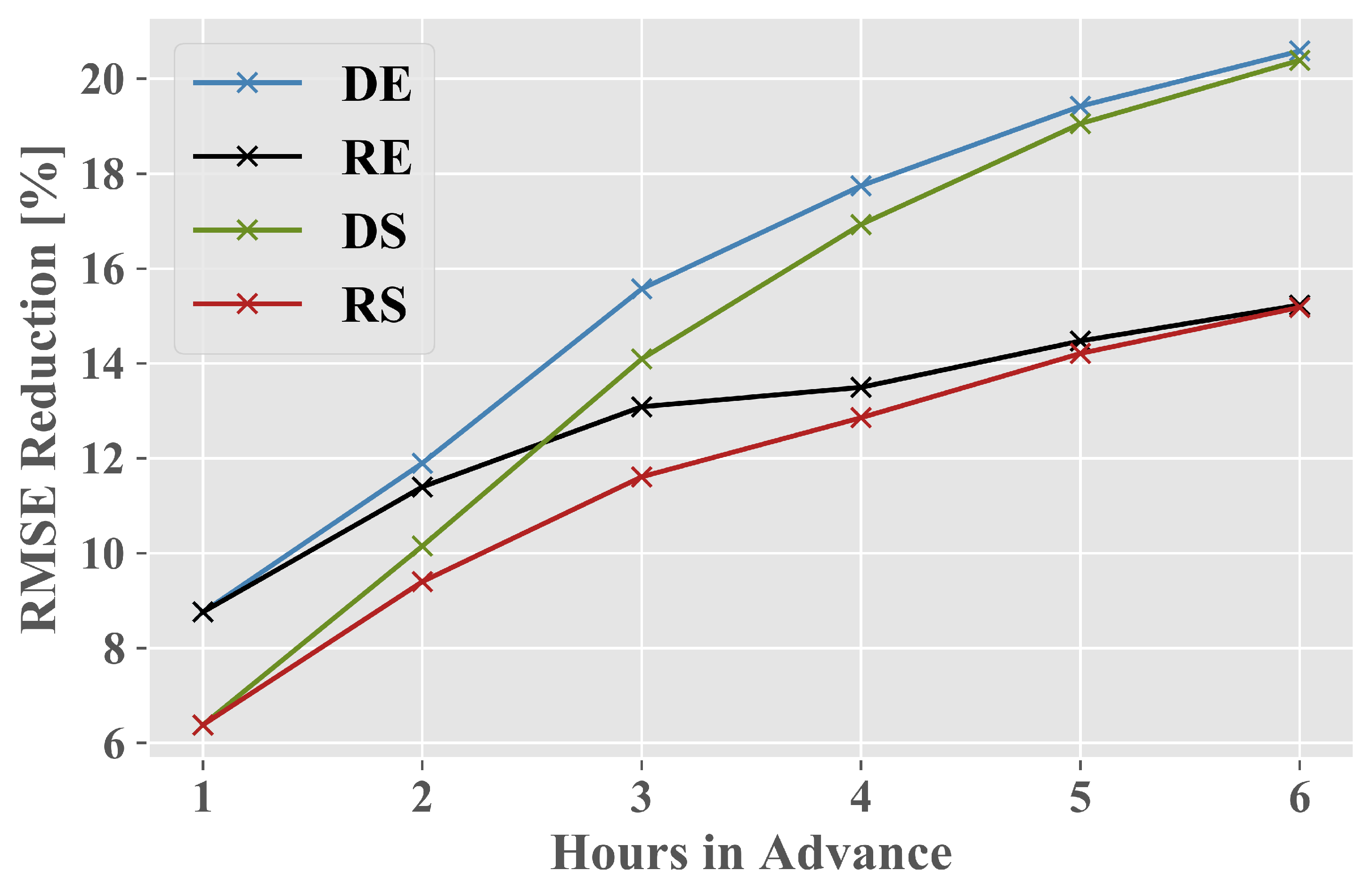
As can be seen in Figure 7, DE outperformed all other modeling strategies for forecasts two to six hours in advance at the SGP C1 site. Forecasting improvement was much greater than that seen at the FINO1 site, likely due to the smaller influence of wind farms which can complicate flow field features. All modeling strategies showed greater improvement with forecasting timescale, with the DE and DS methods decreasing RMSE by as much as 20% below that of the persistence method. Testing metrics may be found at the bottom of Table A2 in Appendix B.
Unlike FINO1, the SGP C1 results suggest that direct modeling is a vastly superior RF forecasting strategy at this site. While RE is superior to DS for forecasts one to two hours in advance, DS quickly overtakes RE and is almost equivalent to DE when used to forecast five or six hours in advance. The fact that direct modeling outperforms its recursive counterpart for all forecasting timesteps corroborates the results of Ahmed and Khalid [12], who found that direct forecasting outperformed recursive forecasting for all multi-step predictions. This may be due to the propagation of error in recursive modeling [31]. Each hourly forecast accumulates a small amount of error, whether it be from inaccurate initial representation of atmospheric variables (initialization error) or misrepresentation of the atmospheric system by the model itself (modeling error). This is similar to error propagation within NWP models, except ML models lack a foundation in atmospheric physics. Conversely, direct multi-step forecasting error partially originates from bypassed atmospheric dynamics that take place between the current time ( τ ) and the forecasted time ( τ + n , n 1 ). As is described in both Wang et al. [11] and Ahmed and Khalid [12], a more optimal modeling strategy is likely the creation of a hybrid model which combines the recursive and direct methodologies.
The SGP C1 results are not obviously partitioned based on the question of differenced vs. absolute target variables, particularly when forecasting more than three hours in advance. This is likely due to the relatively low IAV (3.5%) at the SGP C1 site over the analysis period. This is less than half of that seen at the FINO1 site (8.0%), thereby reducing the likelihood that the training and testing datasets have drastically different U distributions (Figure 2c,d). These results imply that target variable selection (U vs. ε ) is not as crucial for multi-step forecasting when IAV is low. However, forecasts of ε still outperform those of U at a negligible additional computational expense, signifying that it is not only a more robust strategy for both high and low-IAV regions, but can also provide slight improvements for ML forecasting models.
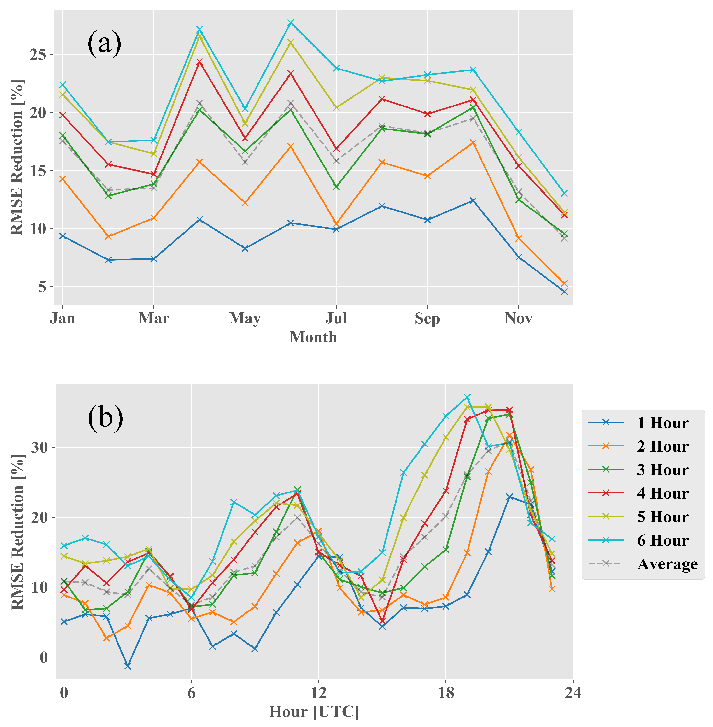
The DE model improvement at SGP C1 shows less seasonality than that at FINO1 (Figure 8a). There is a seasonal trend in absolute model performance for both the persistence and DE models, as both models generate the highest RMSE values in the late winter/early spring and the lowest in the fall (not shown). However, even with this seasonal trend, the DE model vastly outperforms the persistence model throughout the entire year.
Similar to the FINO1 findings, there is a clear diurnal pattern at the SGP C1 site (Figure 8b). The DE model reduces RMSE, on average, by ∼30% in the afternoon (local time = UTC–0600 h) at the peak of daytime convection. The nocturnal boundary layer at the SGP C1 site is invariably topped by a low-level jet (LLJ) [32,33] which has an impact on wind energy resources [34]. The jet’s elevation peaks at approximately 500 m above ground level [35]. The LLJ assists in the development of an extremely stable atmospheric condition at the SGP C1 site, conditions which the model struggles to predict. One reason for the model’s poor performance could be the lack of domain-specific input features such as LLJ elevation, Monin-Obukhov length, and Richardson number that would help the ML model accurately assess atmospheric stability [9].

3.2.2. Training Data Availability

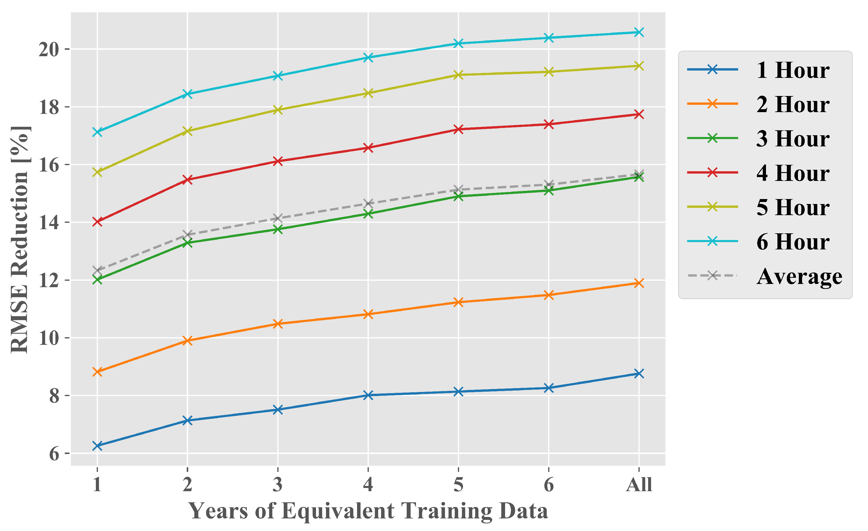
The effect of training data availability at the SGP C1 site, seen in Figure 9, follows a similar pattern to that seen at the FINO1 site, although there are some discrepancies. The largest jump in RMSE improvement is seen when the amount of training data is increased from one to two equivalent years. The average improvement trend is relatively monotonic, with the RF model slowly improving due to an increased pool of training data. It is noteworthy that the model improves even as the pool of training data expands up to approximately eight equivalent years. Testing metrics may be found in Table A3 in Appendix B.
The discrepancies between the SGP C1 and FINO1 availability results, specifically when using five or more equivalent years of training data, are likely due to their respective surroundings. As was stated in Section 3.1.2, multiple wind farms were built near the FINO1 site during the reported data collection period, whereas the only such farm near SGP C1 likely has no (or a nearly negligible) effect on the prediction. The SGP C1 site also has a low IAV (3.5%), meaning that climatological flow patterns are relatively steady on an annual scale (Figure 1b). The lack of anthropogenic flow alterations and low IAV means that, at the SGP C1 site, information from a decade prior is likely still relevant for RF wind speed forecasting. While all curves in Figure 9 flatten as more training data is added, none appear to reach a stable asymptote, indicating that small improvements may still be observed if the training set is expanded to encompass a decade or more of measurements. However, it is worth noting that the DE prediction for both sites improves <5% when given the entire training set compared to a single equivalent year of training data, suggesting that the DE model provides robust predictions even when data availability is low.

4. Conclusions

This paper concludes that hybrid persistence–RF modeling, which utilizes persistence error ε as the target variable, is a more optimal forecasting strategy than using RF as a standalone model. Such a transformation of the target variable not only safeguards against wind speed IAV by providing a more consistent target variable distribution, it also comes at negligible computational expense. Likewise, for multi-step forecasts, it is likely beneficial to directly forecast multiple steps ahead rather than relying on a recursive process that leads to propagation of error. This is a valuable finding, as recursive models require far more computing power (a model must be created to calculate every variable at each timestep) than their direct counterparts for single-output models such as RF. The authors expect both findings to hold for various other ML models, but further studies are required to confirm this hypothesis.
While the findings were quantitatively disparate for the two sites, they showed qualitative solidarity. The hybrid persistence–RF models predicting ε outperformed their standalone counterparts in all study cases and proved to be especially useful in a region with high IAV. Previous studies [10,36] have shown that hybrid and ensemble methodologies tend to outperform their individual modeling components, and yet such methodologies may be overlooked due to their increased complexity, leading to potentially indecipherable (black-box) models. This simple differencing technique, however, requires negligible additional computational power and allows for simple deconstruction of its individual modeling components, making it an easy, comprehensible technique that can be used within the wind energy field.
Direct forecasting proved to be superior to recursive forecasting, particularly with an increasing number of forecasting timesteps. While direct forecasting yields potentially minimal benefits compared to its recursive counterpart (particularly when forecasting two to three timesteps ahead), it can be far less computationally expensive for models incorporating exogenous inputs. Recursive statistical or ML models utilizing exogenous inputs require the creation of a forecasting model for each non-temporal input feature (unless the model has a multivariate output vector). The computational requirements for such models therefore increase proportionally with the number of input features. By utilizing a direct forecasting technique, we bypass these additional complications and instead create a single model which makes a direct prediction of our desired result.
Finally, the relationship between training data availability and model performance shows that, as expected, the model improves with additional input samples. However, this improvement appears to be highly situational. The FINO1 results show that training data collected during previous flow regimes (e.g., measurements taken downstream of free flow vs. obstructed flow) is potentially nugatory or, at worst, deleterious for an ML model. However, as the SGP C1 results show, data collected as much as a decade prior to the testing period can still improve model performance. While more representative training data is always preferred, it is comforting to know that providing the DE model with a single equivalent year of training data yields similar results ( < 5 % decrease in forecasting accuracy) as the DE model when provided with almost a decade of training data. The model’s ability to (relatively accurately) forecast wind speeds using only a year of information from a decade prior could potentially allow for timely forecasting capabilities for newly constructed wind farms and rapid assessment of changes in the local micro-climate due to natural (e.g., wildfires) or anthropogenic (e.g., wind farm construction) causes.
The findings of this study are expected to assist the general construction and use of RF models for multi-step wind speed forecasting. While it is useful to know that the DE model is the best of all tested modeling strategies, this investigation is only the tip of the iceberg with regard to discerning optimal ML strategies for multi-step wind speed forecasting. Future investigations will examine the effects of decomposition methods such as empirical mode decomposition on RF prediction accuracy [37]. Many more questions still require investigation, including:
  • Quantification of the effect of endogenous models vs. models which utilize exogenous variables
  • Which exogenous variables are most beneficial for multi-step wind speed forecasting
  • Which ML models, when used both individually and within an ensemble framework, are best suited for wind speed forecasting
  • Whether the optimal ML modeling methodology changes with the forecasting timescale (e.g., are certain models and modeling strategies better suited for very short-term forecasting while others are better suited for medium/long term forecasting?)
Many studies approach these questions but tend to focus on optimization of a specific model for a specific location, topography, etc. This has led to modeling frameworks which, while powerful, tend to be site-specific and computationally expensive, two of the primary problem areas which ML modeling was supposed to mitigate. In the authors’ opinions, ML modeling strategies must become more generalizable in order to achieve their prodigious potential, with future investigations focusing on the effects of tweaking the modeling methodology (on both a small and large scale) to make the models widely applicable for a variety of terrains and climatologies. The future of ML in the wind energy sector is exciting, and we hope that this investigation will prompt further advancements that benefit the wind energy industry as a whole.

Author Contributions

Conceptualization, D.V.; Data curation, R.K.; Formal analysis, D.V.; Funding acquisition, H.J.S.F.; Investigation, D.V.; Methodology, D.V. and R.K.; Supervision, R.K. and H.J.S.F.; Validation, R.K. and H.J.S.F.; Writing—original draft, D.V.; Writing—review & editing, R.K., T.S. and H.J.S.F. All authors have read and agreed to the published version of the manuscript.

Funding

This research was funded by the National Science Grant numbers AGS-1565535 and AGS-1921554, Wayne and Diana Murdy Endowment at University of Notre Dame, and Dean’s Graduate Fellowship for D.V.

Acknowledgments

This work in part was supported by National Science Foundation Awards AGS-1565535 and AGS-1921554 and the Dean’s Graduate Fellowship for D.V. The Pacific Northwest National Laboratory is operated for the DOE by Battelle Memorial Institute under Contract DE-AC05-76RLO1830. Thanks to the Bundesministerium für Wirtschaft und Energie, Federal Ministry for Economic Affairs and Energy (BMWi), the Projekttraeger Juelich (PTJ), and Markus Kreklau for FINO1 data collection and access. SGP C1 data were obtained from the Atmospheric Radiation Measurement (ARM) user facility, a U.S. Department of Energy (DOE) Office of Science user facility managed by the Biological and Environmental Research Program.

Conflicts of Interest

The authors declare no conflict of interest.

Abbreviations

The following abbreviations are used in this manuscript:
MLMachine learning
ARMAtmospheric Radiation Measurement
SGPSouthern Great Plains
SGP C1Southern Great Plains central facility site
NWPNumerical Weather Prediction
RFRandom forest
MSEMean squared error
MSLAbove mean sea level
THWAPSTemperature, humidity, wind, and pressure sensors
RSRecursive standalone RF model
RERecursive RF model predicting persistence modeling error
DSDirect standalone RF model
DEDirect RF model predicting persistence modeling error
RMSERoot mean squared error
IAVInter-annual variability
LLJLow-level jet
PDFProbability density function

Appendix A. Data Availability

The amount of training and testing data changed slightly with the number of hours forecasted in advance, as can be seen in Table A1. FINO1 training and testing data ranged from January 2004–August 2017 and August 2017–August 2018, respectively. SGP C1 training and testing data ranged from January 2003–November 2013 and November 2013–December 2014, respectively. The testing datasets span almost exactly one year, thereby minimizing seasonal bias within the testing results (although the effects of IAV still persist). Annual and monthly training data availability can be seen in Figure A1. There was zero data availability for four years of the FINO1 analysis period (2008, 2009, 2013, 2014).
Table A1. Number of training and testing samples for each forecast. Number of overall samples decreased slightly with forecasting timescale due to decreasing data availability.
Samples
FINO1SGP C1
Hours in AdvanceTrainingTestingTrainingTesting
160,984677773,0128113
259,402660165,2807254
358,918654763,0467006
458,536650562,4276937
558,203646861,9966889
657,904643461,6356849
Figure A1. (a,c) Annual and (b,d) monthly training data availability for the FINO1 (top row) and SGP C1 (bottom row) datasets for a one-hour forecast. The amount of training data changed with the number of hours forecasted in advance, but all tests (except those testing the effects of reduced training data) had over 57,000 training samples and 6400 testing samples.
Energies 13 05488 g0a1

Appendix B. Testing Results

Table A2 shows the RMSE obtained by each of the four modeling strategies as well as that obtained by the persistence method at both sites. DE outperforms all other methods analyzed in this study for forecasts two to six hours in advance. Table A3 shows the RMSE obtained by the DE model when given varying amounts of training data at both sites.
Table A2. RMSE (m s 1 ) obtained by the four modeling strategies tested as well as the persistence model for hourly forecasts one to six hours in advance.
FINO1
Hours in Advance
Model123456
Persistence0.8531.2791.5921.8392.0652.247
DE0.8221.2221.5061.7351.9322.094
RE0.8221.2241.5111.7431.9462.111
DS0.8381.2461.5331.7651.9642.127
RS0.8381.2441.5331.7681.9702.137
SGP C1
Hours in Advance
Model123456
Persistence0.7991.2021.4901.7191.9002.055
DE0.7291.0591.2581.4141.5311.632
RE0.7291.0651.2951.4871.6251.742
DS0.7481.0801.2801.4281.5381.636
RS0.7481.0891.3171.4981.6301.743
Table A3. RMSE (m s 1 ) obtained by the DE strategy given varying amounts of training data when forecasting hourly wind speed one to six hours in advance.
FINO1
Years of Data
Hours in Advance123456All
10.8480.8370.8310.8240.8240.8220.822
21.2621.2491.2381.2241.2241.2221.222
31.5551.5411.5211.5061.5041.5061.506
41.7821.7731.7471.7401.7341.7361.735
51.9821.9691.9491.9441.9301.9331.932
62.1532.1332.1172.1092.0912.0972.094
SGP C1
Years of Data
Hours in Advance123456All
10.7490.7420.7390.7350.7340.7330.729
21.0961.0831.0761.0721.0671.0641.059
31.3111.2921.2851.2771.2681.2651.258
41.4781.4531.4421.4341.4231.4201.414
51.6011.5741.5601.5491.5371.5351.531
61.7031.6761.6631.6501.6401.6361.632

References

  1. Feng, J. Artificial Intelligence for Wind Energy (AI4Wind): A State of the Art Report; Technical Report; Technical University of Denmark, Department of Wind Energy: Lyngby, Denmark, 2019. [Google Scholar]
  2. Dupré, A.; Drobinski, P.; Alonzo, B.; Badosa, J.; Briard, C.; Plougonven, R. Sub-hourly forecasting of wind speed and wind Energy. Renew. Energy 2020, 145, 2373–2379. [Google Scholar] [CrossRef]
  3. Soman, S.S.; Zareipour, H.; Malik, O.; Mandal, P. A review of wind power and wind speed forecasting methods with different time horizons. In Proceedings of the North American Power Symposium 2010, Arlington, TX, USA, 26–28 September 2010; IEEE: Piscataway, NJ, USA, 2010; pp. 1–8. [Google Scholar]
  4. Lahouar, A.; Slama, J.B.H. Hour-ahead wind power forecast based on random forests. Renew. Energy 2017, 109, 529–541. [Google Scholar] [CrossRef]
  5. Feng, C.; Cui, M.; Hodge, B.M.; Zhang, J. A data-driven multi-model methodology with deep feature selection for short-term wind forecasting. Appl. Energy 2017, 190, 1245–1257. [Google Scholar] [CrossRef] [Green Version]
  6. Niu, D.; Pu, D.; Dai, S. Ultra-short-term wind-power forecasting based on the weighted random forest optimized by the niche immune lion algorithm. Energies 2018, 11, 1098. [Google Scholar] [CrossRef] [Green Version]
  7. Sun, Z.; Sun, H.; Zhang, J. Multistep wind speed and wind power prediction based on a predictive deep belief network and an optimized random forest. Math. Probl. Eng. 2018, 2018. [Google Scholar] [CrossRef] [Green Version]
  8. Shi, K.; Qiao, Y.; Zhao, W.; Wang, Q.; Liu, M.; Lu, Z. An improved random forest model of short-term wind-power forecasting to enhance accuracy, efficiency, and robustness. Wind. Energy 2018, 21, 1383–1394. [Google Scholar] [CrossRef]
  9. Vassallo, D.; Krishnamurthy, R.; Fernando, H.J.S. Utilizing Physics-Based Input Features within a Machine Learning Model to Predict Wind Speed Forecasting Error. Wind. Energy Sci. Discuss. 2020, 1–18. [Google Scholar] [CrossRef]
  10. Haupt, S.E.; Mahoney, W.P.; Parks, K. Wind power forecasting. In Weather Matters for Energy; Springer: Berlin/Heidelberg, Germany, 2014; pp. 295–318. [Google Scholar]
  11. Wang, J.; Song, Y.; Liu, F.; Hou, R. Analysis and application of forecasting models in wind power integration: A review of multi-step-ahead wind speed forecasting models. Renew. Sustain. Energy Rev. 2016, 60, 960–981. [Google Scholar] [CrossRef]
  12. Ahmed, A.; Khalid, M. An intelligent framework for short-term multi-step wind speed forecasting based on Functional Networks. Appl. Energy 2018, 225, 902–911. [Google Scholar] [CrossRef]
  13. Breiman, L. Random forests. Mach. Learn. 2001, 45, 5–32. [Google Scholar] [CrossRef] [Green Version]
  14. Loh, W.Y. Classification and regression tree methods. Wiley Statsref. Stat. Ref. Online 2014. [Google Scholar] [CrossRef]
  15. Pedregosa, F.; Varoquaux, G.; Gramfort, A.; Michel, V.; Thirion, B.; Grisel, O.; Blondel, M.; Prettenhofer, P.; Weiss, R.; Dubourg, V.; et al. Scikit-learn: Machine Learning in Python. J. Mach. Learn. Res. 2011, 12, 2825–2830. [Google Scholar]
  16. James, G.; Witten, D.; Hastie, T.; Tibshirani, R. An Introduction to Statistical Learning; Springer: Berlin/Heidelberg, Germany, 2013; Volume 112. [Google Scholar]
  17. Neumann, T.; Nolopp, K. Three years operation of far offshore measurements at FINO1. DEWI Mag. 2007, 30, 42–46. [Google Scholar]
  18. Westerhellweg, A.; Neumann, T.; Riedel, V. Fino1 mast correction. Dewi Mag. 2012, 40, 60–66. [Google Scholar]
  19. Sisterson, D.; Peppler, R.; Cress, T.; Lamb, P.; Turner, D. The ARM southern great plains (SGP) site. Meteorol. Monogr. 2016, 57, 6.1–6.14. [Google Scholar] [CrossRef]
  20. Atmospheric Radiation Measurement (ARM) user facility. Temperature, Humidity, Wind, and Pressure Sensors (THWAPS). In 2003-01-01 to 2014-12-31, Southern Great Plains (SGP) Central Facility, Lamont, OK (C1); Kyrouac, J., Ermold, B., Eds.; ARM Data Center: Cambridge, UK, 1999. [Google Scholar] [CrossRef]
  21. Ritsche, M. Temperature, Humidity, Wind and Pressure Sensors (THWAPS) Handbook; Technical report; DOE Office of Science Atmospheric Radiation Measurement (ARM) Program: Cambridge, UK, 2011. [Google Scholar]
  22. Chatfield, C.; Prothero, D. Box-Jenkins seasonal forecasting: Problems in a case-study. J. R. Stat. Soc. Ser. 1973, 136, 295–315. [Google Scholar] [CrossRef]
  23. Dickey, D.A.; Pantula, S.G. Determining the order of differencing in autoregressive processes. J. Bus. Econ. Stat. 1987, 5, 455–461. [Google Scholar]
  24. Hyndman, R.J.; Athanasopoulos, G. Forecasting: Principles and Practice; OTexts: Melbourne, Australia, 2018. [Google Scholar]
  25. Bontempi, G.; Taieb, S.B.; Le Borgne, Y.A. Machine learning strategies for time series forecasting. In European Business Intelligence Summer School; Springer: Berlin, Heidelberg, Germany, 2012; pp. 62–77. [Google Scholar]
  26. Pryor, S.C.; Shepherd, T.J.; Barthelmie, R.J. Interannual variability of wind climates and wind turbine annual energy production. Wind. Energy Sci. 2018, 3, 651. [Google Scholar] [CrossRef] [Green Version]
  27. Brower, M. Wind Resource Assessment: A Practical Guide to Developing a Wind Project; John Wiley & Sons: Hoboken, NJ, USA, 2012. [Google Scholar]
  28. McGaughey, G.; Walters, W.P.; Goldman, B. Understanding covariate shift in model performance. F1000Research 2016, 5, 6. [Google Scholar] [CrossRef]
  29. Fruehmann, R.K.; Neumann, T. Wake effects at FINO 1–new observations since the construction of Trianel Borkum & Borkum Riffgrund I wind farms. In Proceedings of the WindEurope Summit 2016, Hamburg, Germany, 27–30 September 2016; EWEA: Brussels, Belgium, 2016. [Google Scholar]
  30. Westerhellweg, A.; Cañadillas, B.; Kinder, F.; Neumann, T. Wake measurements at Alpha Ventus–dependency on stability and turbulence intensity. J. Phys. Conf. Ser. Iop Publ. 2014, 555, 012106. [Google Scholar] [CrossRef] [Green Version]
  31. Taieb, S.B.; Bontempi, G.; Atiya, A.F.; Sorjamaa, A. A review and comparison of strategies for multi-step ahead time series forecasting based on the NN5 forecasting competition. Expert Syst. Appl. 2012, 39, 7067–7083. [Google Scholar] [CrossRef] [Green Version]
  32. Whiteman, C.D.; Bian, X.; Zhong, S. Low-level jet climatology from enhanced rawinsonde observations at a site in the southern Great Plains. J. Appl. Meteorol. 1997, 36, 1363–1376. [Google Scholar] [CrossRef]
  33. Song, J.; Liao, K.; Coulter, R.L.; Lesht, B.M. Climatology of the low-level jet at the southern Great Plains atmospheric boundary layer experiments site. J. Appl. Meteorol. 2005, 44, 1593–1606. [Google Scholar] [CrossRef]
  34. Wimhurst, J.J.; Greene, J.S. Oklahoma’s future wind energy resources and their relationship with the Central Plains low-level jet. Renew. Sustain. Energy Rev. 2019, 115, 109374. [Google Scholar] [CrossRef]
  35. Berg, L.K.; Riihimaki, L.D.; Qian, Y.; Yan, H.; Huang, M. The low-level jet over the southern Great Plains determined from observations and reanalyses and its impact on moisture transport. J. Clim. 2015, 28, 6682–6706. [Google Scholar] [CrossRef]
  36. Opitz, D.; Maclin, R. Popular ensemble methods: An empirical study. J. Artif. Intell. Res. 1999, 11, 169–198. [Google Scholar] [CrossRef]
  37. Bokde, N.; Feijóo, A.; Villanueva, D.; Kulat, K. A review on hybrid empirical mode decomposition models for wind speed and wind power prediction. Energies 2019, 12, 254. [Google Scholar] [CrossRef] [Green Version]
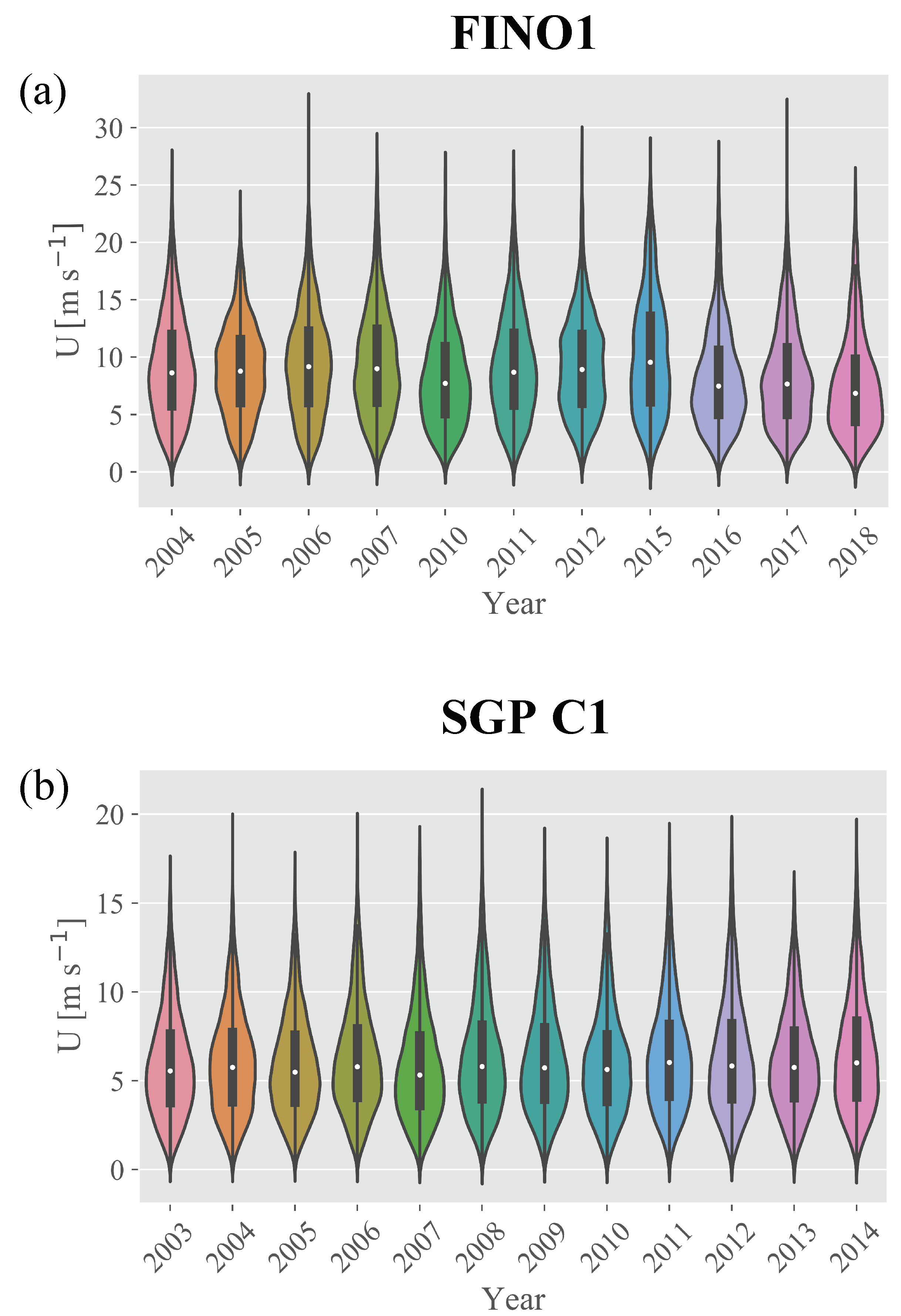
Figure 1. Violin plot of annual wind speed distribution for all training and testing data at the (a) FINO1 and (b) Southern Great Plains (SGP) C1 sites. Years without any data availability are removed for clarity.
Energies 13 05488 g001
Figure 2. Probability distribution functions (PDFs) of (a,c) U and (b,d) ε for the FINO1 (top row) and SGP C1 (bottom row) datasets. Red shading represents training set distributions, while blue shading represents testing set distributions.
Energies 13 05488 g002
Figure 3. Illustration of the difference between the recursive and direct models for a two-step prediction. Gray blocks represent known data, or data from periods τ 1 and τ that may be used as inputs. Green blocks represent predictions made by the models. The empty dashed box under direct forecasting represents the time period that is skipped by the two-step direct prediction.
Energies 13 05488 g003
Figure 4. Reduction in root mean squared error (RMSE) obtained by all four models compared to the persistence model at the FINO1 site. Blue, black, green, and red lines denote the direct error (DE), recursive error (RE), direct standalone (DS), and recursive standalone (RS) strategies, respectively.
Energies 13 05488 g004
Figure 5. Reduction in RMSE obtained by the DE model at FINO1 as partitioned by (a) month and (b) hour of the day (local time = UTC + 0100 h). Solid lines represent forecasts one to six hours in advance, while the dashed line represents the average over all forecasts.
Energies 13 05488 g005
Figure 6. Reduction in RMSE obtained by the DE modeling strategy compared to the persistence model based on the amount of training data available at the FINO1 site. Solid colored lines indicate the number of hours in advance for forecasting, while the dashed gray line indicates the average of all colored lines.
Energies 13 05488 g006
Figure 7. Similar to Figure 4 except data are taken from the SGP C1 site.
Energies 13 05488 g007
Figure 8. Similar to Figure 5 except data are taken from the SGP C1 site. RMSE reduction is partitioned by (a) month and (b) hour of the day (local time = UTC–0600 h).
Energies 13 05488 g008
Figure 9. Similar to Figure 6 except data are taken from the SGP C1 site.
Energies 13 05488 g009
Table 1. Input variable statistics for the FINO1 and SGP C1 training datasets. θ 1 and θ 2 represent the North-South and East-West components of wind direction, respectively.
FINO1
U [m s 1 ] T I θ 1 θ 2 T [C]
Mean8.990.09−0.22−0.2811.31
St. Dev.4.370.050.630.695.81
Max31.480.501.001.0041.92
Min0.240.00−1.00−1.00−6.67
SGP C1
U [m s 1 ] T I θ 1 θ 2 T [C]
Mean6.200.19−0.230.1319.79
St. Dev.2.950.140.780.578.39
Max20.340.981.001.0044.17
Min0.240.00−1.00−1.00−8.11
Sample Availability: Samples of the data and code may be found at https://github.com/dvassall/WS_Forecasting_Strategies_Sample.
Publisher’s Note: MDPI stays neutral with regard to jurisdictional claims in published maps and institutional affiliations.