A Decoupling Rolling Multi-Period Power and Voltage Optimization Strategy in Active Distribution Networks

Abstract

With the increasing penetration of distributed photovoltaics (PVs) in active distribution networks (ADNs), the risk of voltage violations caused by PV uncertainties is significantly exacerbated. Since the conventional voltage regulation strategy is limited by its discrete devices and delay, ADN operators allow PVs to participate in voltage optimization by controlling their power outputs and cooperating with traditional regulation devices. This paper proposes a decoupling rolling multi-period reactive power and voltage optimization strategy considering the strong time coupling between different devices. The mixed-integer voltage optimization model is first decomposed into a long-period master problem for on-load tap changer (OLTC) and multiple short-period subproblems for PV power by Benders decomposition algorithm. Then, based on the high-precision PV and load forecasts, the model predictive control (MPC) method is utilized to modify the independent subproblems into a series of subproblems that roll with the time window, achieving a smooth transition from the current state to the ideal state. The estimated voltage variation in the prediction horizon of MPC is calculated by a simplified discrete equation for OLTC tap and a linearized sensitivity matrix between power and voltage for fast computation. The feasibility of the proposed optimization strategy is demonstrated by performing simulations on a distribution test system.

1. Introduction

The rapid penetration of distributed photovoltaics (PVs) in active distribution networks (ADNs) has considerably challenged the operation mode of the traditional grid [1]. Some research indicates that one of the major constraints for promoting PV integration into ADNs is voltage stability [2,3]. The voltage at the end of feeder will rise if the intermittent production of PV generation causes power flow reversal [4,5]. Since undesirable voltage violations may cause serious negative effects [6], an appropriate effective reactive power and voltage strategy is required to solve these problems.

The on-load tap changer (OLTC) in distribution networks is considered to be a typical control device to prevent the violations of voltages, which keeps the substation secondary bus voltage constant by adjusting the tap position [7]. However, due to physical constraints and low cost benefit ratios, it cannot change flexibly to achieve real-time adjustment [8,9]. Recently, the continuous, quick and frequent reactive power outputs of distributed generation are appealing to mitigate voltage violations and fluctuations [10,11], which avoids adding extra voltage devices and reactive compensators in ADN. The authors of [12,13] presented an optimized decentralized control approach for each PV inverter based on voltage sensitivity analysis by implementing the control action at the point of common coupling (PCC) [14] as one of ancillary services to the ADN. A multi-mode adaptive local reactive power control method based on Q(P) characteristics is discussed in [15] considering control parameter optimization. Reference [16] proposed a combination of centralized-remote control and local-decentralized control to ensure that the nodal voltages remain within regulatory limits. Although these studies have fully demonstrated that distributed PVs have the ability to enhance power quality as well as reliability of the system [17], their reactive outputs are limited by capacity and power factor. Moreover, the line equivalent impedance directly affects the voltage regulation. the R/X ratio determines the influence of the active power and reactive power injected by distributed generation on the node voltage [18]. For the low-reactance cables, it is more difficult to try to keep the voltage within the allowable range by adjusting the reactive power output of distributed generations. The fluctuation of PV active power output greatly affects the node voltage. When serious violations occur, it is insufficient to correct serious violations by distributed PVs alone, which requires cooperation with traditional adjustment devices [19]. It follows that the reactive power and voltage optimization model of ADN is a complex mixed integer nonlinear programming (MINP) problem, not only dealing with continuous control variables such as of PV outputs, but also handling discrete variables such as OLTC tap changes. In [20,21,22], a control method for coordinating the operation of OLTC and distributed generations (DGs) based on the initial optimal power flow (OPF) calculation in order to maintain the load end voltage of the feeder within the allowed band. The authors of [23,24] incorporated a semi-definite power flow relaxation to tackle such complex problems, while [25,26] decomposed the problem into subproblems by Benders decomposition method and alternate direction method of multipliers respectively. In [27,28,29,30], the discrete variables in optimization models are relaxed into continuous variables and then rounded to close integers. However, these solutions are the static optimization results, regardless of the strong time coupling between the adjustments of different devices. The authors in [31] proposed a two-stage dynamic coordination dispatch method based on the Haar wavelet transform to adjust the OLTC tap position and the reactive power of distributed generation. [32] implemented another two-stage dynamic reactive power dispatch method, which first performed a day-ahead dispatch plan for switched capacitor banks and OLTCs by Heuristic search, and then recalibrated the intra-day dispatch results of PVs. These two-stage methods mentioned pre-optimize discrete devices in advance without considering the interaction between OLTC tap changes and PV outputs. Consequently, the pre-planned scheduling may have large errors and lose dynamic optimality.

Furthermore, previous research has drawn attention to the solutions of PV generation uncertainties. In fact, most optimal dispatch methods based on the predicted scenario can only work in shorter periods, since accurate weather and load forecasts are only valid for a limited period in advance. A multi-step optimization method based on the model predictive control (MPC) principle has been verified to be well suited for this issue by determining the appropriate prediction horizon and control horizon [33,34]. Solving the rolling optimization problems of specific horizons can achieve a dynamic transition from the measured to the target values, which is different from single step optimizations. Notably, varying the horizon of prediction and control has a significant impact on the optimal operation of the current time window. The authors in [35] developed a planning method that leverages MPC principle to decide the optimal location and size of storage devices in ADN. [36] proposed a control strategy based on MPC to balance the intermittency of PV outputs by little adjustments of conventional generation and load, as well as the storage devices. In [9], an MPC-based corrective control is utilized to correct voltages out of limits by solving the OLTC voltage set-point and PV outputs. However, due to the different operation characteristics of various devices, the requirement of subdividing the control horizon was ignored. On the one hand, limited forecasts cannot support the long-period scheduling. On the other hand, frequent short horizons will increase the modeling time and make the optimization problem computationally intractable. Table 1 gathers the main features of ADN optimization methods found in the existing literature.

Table 1. Summary of the literature related to ADN optimization method.

Devices	Reference	Method/Algorithm	Remarks
OLTC	[7]	Mixed integer nonlinear programming (MINP)	Disadvantages: due to physical constraints and low cost benefit ratios, OLTC cannot change flexibly to achieve real-time adjustment
DG	[12,13]	Decentralized control based on voltage sensitivity	Advantages: The continuous, quick and frequent reactive power outputs of DGs avoids adding extra voltage devices and reactive compensators. Disadvantages: DG reactive outputs are limited by capacity and power factor. It is insufficient to correct serious violations by DGs alone.
	[15]	A multi-mode adaptive local control method based on Q(P) characteristics
	[16]	a combination of centralized remote control and local decentralized control
DG, OLTC	[20,21,22]	Optimal power flow (OPF) calculation	Disadvantages: These solutions are the static optimization results, regardless of the strong time coupling between the adjustments of different devices.
	[23,24]	Semi-definite relaxation
	[25,26]	Benders decomposition
	[27,28,29,30]	Relaxing discrete variables into continuous variables and rounding to close integers.
	[31,32]	Two-stage dynamic coordination dispatch	Advantages: the dynamic optimization results. Disadvantages: The pre-planned scheduling may have large errors and lose dynamic optimality.
Storage device, OLTC, DG	[9,35,36]	Model predictive control (MPC)	Advantages: Rolling optimization of the specific horizon can achieve a dynamic transition from the measured to the target values. Disadvantages: The requirement of subdividing the control horizon for different devices is ignored.

In this paper, a decoupling rolling multi-period (DRM) reactive power and voltage optimization method of ADN is proposed. The main contribution is two-fold. First, for the mixed-integer reactive power and voltage optimization problem, we utilize Benders decomposition algorithm to decouple the coordination between discrete OLTC tap changers and continuous PV power outputs in the original problem into the master problem and the subproblem. In terms of time, our method designs the master problem of OLTC tap as a long-period optimization model, and the subproblem of PV power is a series of short-period optimization models. This allows us to address PV and load uncertainty by dividing the fluctuating PV and load condition into various short-period scenarios, avoiding frequent OLTC tap changes. Secondly, these short-period independent subproblems are incorporated into the MPC strategy and solved on a rolling basis, because predicting PV power generation of all short periods in the current time window may lead to large errors and additional adjustment costs. Based on the linearized voltage prediction model, the interrelation between rolling subproblems are considered to realize the gradual evolution of the ideal voltage in a long period, i.e., the prediction and control horizon of MPC. Besides, we present how to formulate Benders decomposition algorithm for this reactive power and voltage optimization problem, including the solution process, achieving the multi-period decoupling rolling optimization effect of different devices.

The rest of the paper is organized as follows: In Section 2, the model of voltage sensitivity is established, as well as the modeling of OLTC and PV. In Section 3, the proposed DRM architecture is illustrated. Section 4 formulates the decomposed optimization models and provides the solution process. In Section 5, the simulation results on the distribution test system are presented to validate the proposed strategy. The conclusions are drawn in Section 6.

2. Modeling of Active Distribution Network

2.1. Sensitivity between Node Voltage and Power

In order to discuss the influence of different voltage regulation devices on nodal voltages, the distribution network can be locally linearized to calculate the sensitivity model (the relationship between nodal voltage deviations and output changes of regulation devices) [37].

Assuming that a distribution network system contains n nodes, the voltage of Node i are expressed in polar coordinate form, ${\dot{V}}_i=V_i{e}^{j{\theta }_i}=V_i\left(cos{\theta }_i+jsin{\theta }_i\right)$. The modified Newton Raphson power flow equation can be simplified as:

$$\left[\begin{array}{c}\Delta P\\ \Delta Q\end{array}\right]=-J\left[\begin{array}{c}\Delta \theta \\ \Delta V\end{array}\right]$$

(1)

where V is the diagonal matrix of voltage amplitude, V = diag(v₁, v₂,…, v_n-1), $\Delta \theta$ and $\Delta V$ are the corrections of the voltage phase angle and voltage amplitude respectively. The Jacobian matrix J is as follows:

$$\mathit{J}=-\left[\begin{array}{cc}\mathit{H}& \mathit{N}\\ \mathit{K}& \mathit{L}\end{array}\right]=\left[\begin{array}{cc}\mathit{V}& \\ & \mathit{V}\end{array}\right]\left\{\left[\begin{array}{cc}\mathit{B}cos\theta & -\mathit{G}cos\theta \\ \mathit{G}cos\theta & \mathit{B}cos\theta \end{array}\right]-\left[\begin{array}{cc}\mathit{G}cos\theta & \mathit{B}sin\theta \\ -\mathit{B}cos\theta & \mathit{G}sin\theta \end{array}\right]\right\}\left[\begin{array}{cc}\mathit{V}& \\ & \mathit{V}\end{array}\right]$$

(2)

where $Bcos\theta$ can be expressed as Equation (3) and the structures of other terms $B\sin \theta$, $Gcos\theta$, and $Gsin\theta$ are similar.

$$Bcos\theta =\left[\begin{array}{lllll}{B}_{1,1}cos{\theta }_{1,1}\hfill & \cdots \hfill & B_{1,j}cos{\theta }_{1,j}\hfill & \cdots \hfill & B_{1,j}cos{\theta }_{1,n}\hfill \\ ⋮\hfill & \ddots \hfill & ⋮\hfill & \hfill & ⋮\hfill \\ B_{i,1}cos{\theta }_{i,1}\hfill & \cdots \hfill & B_{i,j}cos{\theta }_{i,j}\hfill & \cdots \hfill & B_{i,n}cos{\theta }_{i,n}\hfill \\ ⋮\hfill & \hfill & ⋮\hfill & \ddots \hfill & ⋮\hfill \\ B_{n,1}cos{\theta }_{n,1}\hfill & \cdots \hfill & B_{n,j}cos{\theta }_{n,j}\hfill & \cdots \hfill & B_{n,n}cos{\theta }_{n,n}\hfill \end{array}\right]$$

(3)

In the distribution network, the value of ${\theta }_{ij}$ is extremely small, and hence Equation (1) can be further simplified:

$$\left[\begin{array}{cc}B+Q& -G-P\\ G-P& B-Q\end{array}\right]\left[\begin{array}{c}V\Delta \theta \\ \Delta V\end{array}\right]=\left[\begin{array}{c}\Delta P/V\\ \Delta Q/V\end{array}\right]$$

(4)

where P and Q are diagonal matrices, and their diagonal elements are $P_i/V_i^2$ and $Q_i/V_i^2$ respectively. Using the Gaussian elimination method for Equation (4), the sensitivity of nodal voltages and injected power can be calculated as:

$$\Delta V={\left(\left(B+Q\right){\left(G-P\right)}^{-1}\left(B-Q\right)+\left(G+P\right)\right)}^{-1}\Delta P$$

(5)

$$\Delta V=-{\left(\left(G-P\right){\left(B+Q\right)}^{-1}\left(G+P\right)+\left(B+Q\right)\right)}^{-1}\Delta Q$$

(6)

Therefore, the active-voltage sensitivity and reactive-voltage sensitivity can be obtained:

$$S_P={\left(\left(B+Q\right){\left(G-P\right)}^{-1}\left(B-Q\right)+\left(G+P\right)\right)}^{-1}$$

(7)

$$S_{\mathrm{Q}}=-{\left(\left(G-P\right){\left(B+Q\right)}^{-1}\left(G+P\right)+\left(B+Q\right)\right)}^{-1}$$

(8)

2.2. Modeling of OLTC

The discussed OLTC acts on the voltage set-point of the secondary side by changing the tap position. The sensitivity $\mathit{\partial }\mathit{V}/\mathit{\partial }{V}_{tap}$ between nodal voltages and OLTC set-point can be approximated from the solution of two power flow runs with a single tap position difference [9], as follows:

$$S_{tap}=\frac{\mathit{\partial }V}{\mathit{\partial }{V}_{tap}}\approx \frac{\mathit{\partial }\Delta V}{\mathit{\partial }\Delta V_d}$$

(9)

where ΔV_d is voltage variation on the low-voltage side after a OLTC tap change.

2.3. Modeling of PV

In this paper, PVs are set to adjust the reactive power output in the maximum power point tracking (MPPT) mode [7]. The maximum reactive power is limited by active power, power factor and capacity:

$$\left\{\begin{array}{c}{Q}_{m,PV}^{t,max}=P_{m,PV}^{t}tan{\phi }_{max},0<P_{m,PV}^t<P_l\hfill \\ Q_{m,PV}^{t,max}=\sqrt{{\left(S_{m,PV}\right)}^2-{\left(P_{m,PV}^t\right)}^2},P_l<P_{m,PV}^t<P_{max}\end{array}\right.$$

(10)

$$P_l=S_{m,PV}cos{\phi }_{max}$$

(11)

where, $P_{m,PV}^t$ is the PV-m active power output. $Q_{m,PV}^{t,max}$ is the maximum reactive power. $S_{m,PV}$ is the capacity of the PV-m, and ${\phi }_{max}$ is the maximum power factor angle.

3. Decoupling Rolling Multi-Period Architecture

In view of nodal voltage deviations caused by the high proportion of PV generation, the practical implementation is to adjust the OLTC tap positions and the active/reactive power outputs of distributed PVs. The OLTC tap changes are discrete, while the PV power outputs can continuously, quickly, efficiently and accurately respond to operation instructions. The DRM strategy focuses on the temporal interaction between PV and OLTC and explores their cooperation performance on voltage optimization.

The reactive power and voltage optimization model is a MINP problem. The Benders decomposition method is a distributed algorithm that decomposes the original MINP problem into the master problem and the subproblem to obtain the optimal operation results of different controllable devices in the same time step, as shown in Figure 1a. Due to the limitation of OLTC tap changes, the synchronized optimization framework cannot take full advantage of PV flexibility potential. The improved strategy in Figure 1b further decomposes the long-period subproblem of PV reactive power into multiple short-period problems, not only realizing rapid adjustment of PV reactive power, but also avoiding excessive and frequent OLTC tap changes. However, these parallel independent short-period subproblems of PV outputs are still based on the definite long-period PV power generation forecasts. Taking into account the uncertainty of PV power generation prediction, the prediction error becomes larger when the period is longer. The DRM method proposed in this paper rolls a series of short-period subproblems in the prediction horizon to smoothly adjust the PV power, as shown in Figure 1c.

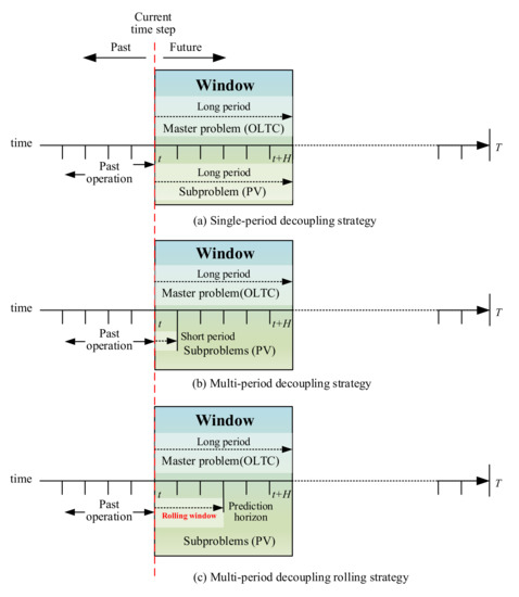
Figure 1. Comparison of the reactive power and voltage optimization strategy framework.

The detailed DRM reactive power and voltage optimization strategy is shown in the Figure 2. The decomposed long-period master problem is to solve OLTC tap changes. Since the increasing number of tap actions will shorten the life of OLTC, the optimization function is to minimize the adjustment cost of OLTC and set at most one tap position change per long period to reduce frequent actions. The voltage is calculated by the sensitivity between the nodal voltage and the OLTC tap in Equation (9) to constrain the range of tap change. After the master problem is solved, the optimal solution of OLTC tap will be sent to subproblems for feasibility verification.

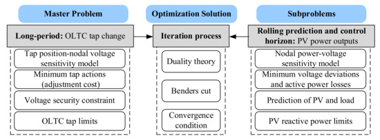
Figure 2. The detailed decomposition diagram of DRM strategy.

The subproblem is a series of PV active power and reactive power optimization problems of the prediction and control horizon considering the constraints of PV power factor and capacity. As the PV capacity limits the effectiveness of reactive power optimization, it is considered to reduce PV active power outputs in critical situations. Compared with the reactive power adjustment costs, the unit cost of PV active power regulation is significantly higher. Based on the MPC algorithm, a voltage prediction model is established from the sensitivity matrix of nodal power and voltage to ensure that the voltage is always in a safe range. Taking the current measured value as the initial state, the time window is rolled to complete the optimal solution in a long period, achieving a dynamic transition to the ideal result and suppressing large fluctuations of the PV reactive power. The first short-period optimal set of PV reactive power instructions is issued and operated to minimize the sum of deviations between the future nodal voltages and the reference voltage.

Based on the iterative solution step of the Benders decomposition method, the global optimal solution of the DRM optimization model can be found [38]. After the master problem is solved, the OLTC tap position result is sent to the corresponding subproblems in the current time window, based on the duality theory. The subproblems implements rolling solution, which feedback the modified Benders cut constraint to the master problem, according to the feasibility verification. Then the master problem is re-solved by adding the new constraint from subproblems. In this way, the master problem and subproblem are iterated repeatedly until the convergence condition is satisfied and the optimal solution is obtained.

4. Reactive Power and Voltage Optimization Model

This section first establishes a common model of the ADN reactive power and voltage optimization problem, which is later decomposed in to the master problem and rolling subproblems according to the DRM method. At last, the solution process is introduced.

4.1. Objective Function

The objective function of the proposed DRM method is composed of three parts, which are the adjustment cost, the voltage deviation and the active power loss. Both OLTC and PV adjustment costs are considered in the objective function:

$$C_{tap}=c_b\Delta N_{tap}^{}{}^2$$

(12)

$$C_{PV}=c_{P,PV}{‖P_{PV}-{\tilde{P}}_{PV}‖}_2^2+c_{Q,PV}{‖\Delta Q_{PV}^{}‖}_2^2$$

(13)

where $P_{PV}$ and ${\tilde{P}}_{PV}$ are the actual output and predicted output of PV active power. $\Delta N_{tap}$ and $\Delta Q_{PV}^{}$ are the variations of OLTC tap and PVs reactive power respectively. $c_b$ and $c_{PV}$ are the unit cost coefficients of OLTC and PVs. Please note that the reactive power adjustment cost of PV is calculated by the PV reactive power output changes, while the PV active adjustment cost is the power loss caused by the PV active power curtailment when necessary.

The nodal voltage deviation is one of the most significant reliability factors and service quality indices [39,40], because it is harmful to the operation life and efficiency of electrical devices when the voltage deviation beyond a reasonable range. The fluctuations of load and PV generation increases the risk of node voltage exceeding the limit. However, considering the node voltage limit as a constraint may lead to the voltages rising to their maximum limits after optimization. Choosing the voltage deviations from the ideal voltage reference $V^{ref}$ as an objective function can remove this problem, as shown in Equations (14). If the voltage deviation of the optimization result is large, the voltage is more likely to exceed the limit:

$$V_{sum,de}={‖V^{}-V^{ref}‖}_2^2$$

(14)

Furthermore, distributed PV generation will affect the power flow direction and change the node voltages. This paper considers minimizing active power losses to improve the economy of ADN operation. The network active power loss can be obtained by:

$$P_{loss}^t={\displaystyle \sum _{i,j}^N{G}_{ij}\left(V_i^2+V_i^2-2V_i{V}_j\cos {\theta }_{ij}\right)}\Delta t$$

(15)

In general, the objective function voltage optimization is established based on the chronological scenario:

$$J^{*}={\displaystyle \sum _{t_l=1}^{N_{T_l}}\left[c_b\Delta N_{tap}^{t_l}{}^2+{\displaystyle \sum _{t_s=1}^{N_{T_s}}\left(c_{Q,PV}{‖\Delta Q_{PV}^{t_l,t_s}‖}_2^2+c_{P,PV}{‖P_{PV}^{t_l,t_s}-{\tilde{P}}_{PV}^{t_l,t_s}‖}_2^2+{‖V^{t_l,t_s}-V^{ref}‖}_2^2+P_{loss}^{t_l,t_s}\right)}\right]}$$

(16)

where t_l and t_s mean the long-period time window and rolling short-period time window, while $N_{T_l}$ is the total number of long periods and $N_{T_s}$ is the total short periods in a long period.

4.2. Constraints

Some following constraints are required to set in the ADN reactive power and voltage optimization model. First, based on the sensitivity model for voltage calculation in Section 1, voltage security of each node should be guaranteed. Besides, the PV reactive power output cannot exceed its configured maximum range. Similarly, the OLTC tap is limited by its maximum tap position, as well as the restriction on tap changes of one action.

4.2.1. Voltage Constraints

The nodal voltages of each short period $V^{t_l,t_s}$ can be estimated by the voltages in the previous period and the predicted variations in the current period with respect to OLTC tap changes $\Delta V_{tap}^{t_l,t_s}$ and PV and load power $\Delta V_{PV,load}^{t_l,t_s}$, as shown in Equations (17) and (18). Then, the nodal voltages should be limited within a safe range:

$$\Delta V_{tap}^{t_l,t_s}=S_{tap}\Delta V_d\Delta N_{tap}^{t_l,t_s}$$

(17)

$$\Delta V_{PV,load}^{t_l,t_s}=S_P\left(\Delta P_{PV}^{t_l,t_s}+\Delta P_{load}^{t_l,t_s}\right)+S_Q\left(\Delta Q_{PV}^{t_l,t_s}+\Delta Q_{load}^{t_l,t_s}\right)$$

(18)

$$V^{t_l,t_s}=V^{t_l,t_s-1}+\Delta V_{tap}^{t_l,t_s}+\Delta V_{PV,load}^{t_l,t_s}$$

(19)

$$V^{\min }\le {\mathit{V}}^{t_l,t_s}\le V^{\max }$$

(20)

where $V^{\min }$ and $V^{\max }$ are the lower limit and upper limit of the voltage amplitude.$\Delta N_{tap}^{t_l,t_s}$ is the OLTC tap position change. $\Delta P_{PV}^{t_l,t_s}$, $\Delta Q_{PV}^{t_l,t_s}$, $\Delta P_{load}^{t_l,t_s}$ and $\Delta Q_{load}^{t_l,t_s}$ are the power variations of PV and load, which can be obtained as follows:

$$\left\{\begin{array}{ll}\Delta N_{tap}^{t_l,t_s}=N_{tap}^{t_l,t_s}-N_{tap}^{t_l-1,t_s}\hfill & if{t}_s=1\\ N_{tap}^{t_l,t_s}=N_{tap}^{t_l,1}\hfill & if{t}_s\ne 1\end{array}\right.$$

(21)

$$\left\{\begin{array}{l}\Delta P_{PV}^{t_l,t_s}=P_{PV}^{t_l,t_s}-P_{PV}^{t_l,t_s-1}\\ \Delta Q_{PV}^{t_l,t_s}=Q_{PV}^{t_l,t_s}-Q_{PV}^{t_l,t_s-1}\end{array}\right.$$

(22)

$$\left\{\begin{array}{l}\Delta P_{load}^{t_l,t_s}=P_{load}^{t_l,t_s}-P_{load}^{t_l,t_s-1}\\ \Delta Q_{load}^{t_l,t_s}=Q_{load}^{t_l,t_s}-Q_{load}^{t_l,t_s-1}\end{array}\right.$$

(23)

It is worth noting that the OLTC tap is only changed once in a long period, which is assumed to occur in the first short period, as in Equation (21). The PV active outputs and load conditions in Equations (22) and (23) are based on the current forecast.

4.2.2. PV Power Constraints

Due to the limitations of PV operation mode and capacity in Equations (10) and (11), the reactive adjustment constraint is:

$$\left\{\begin{array}{l}{P}_{PV}^{\min }\le P_{PV}^{t_l,t_s}\le P_{PV}^{\max }\\ Q_{PV}^{\min }\le Q_{PV}^{t_l,t_s}\le Q_{PV}^{\max }\end{array}\right.$$

(24)

where $Q_{PV}^{\max }$ and $Q_{PV}^{\min }$ are the reactive power up-limit matrix and down-limit matrix. $P_{PV}^{\min }$ and $P_{PV}^{\max }$ are the active power up-limit matrix and down-limit matrix.

4.2.3. OLTC Tap Constraints

The OLTC tap range as a key parameter should be considered, as well as the amplitude of one tap change:

$$N_{tap}^{\min }\le N_{tap}^{t_l}\le N_{tap}^{\max }$$

(25)

$$\Delta N_{tap}^{t_l}\in \left\{0,\pm 1\right\}$$

(26)

where $N_{tap}^{\max }$ and $N_{tap}^{\min }$ are the lower limit and upper limit of the OLTC tap position.

4.3. Model Decomposition

In this section, the Benders decomposition method is used to decompose the original optimization problem into a master problem and several MPC-based rolling subproblems to achieve the decoupling of different action periods, as well as the decoupling of discrete and continuous control variables.

(1)

MPC-Based subproblem

The rolling subproblems are based on the MPC algorithm to solve the optimization problem of short-period continuous control variables, PV active and reactive power outputs. We set a predictive and control horizon consisting of $H_s$ short periods. According to load and PV forecasts in the prediction and control horizon, the optimal operation sequence of PV power outputs can be obtained. The specific subproblem model solved by the k-th iteration is:

$$\begin{array}{c}{J}_{sub}^{t_l,k}\left(\Delta N_{tap}^{t_l,k}\right)=min{\displaystyle \sum _{t_s=1}^{N_{T_s}}}({\displaystyle \sum _{h_s=1}^{H_s}}{c}_{Q,PV}\Vert \Delta {\mathit{Q}}_{PV}^{t_l,t_s}{\Vert }_2^2+c_{P,PV}\Vert {\mathit{P}}_{PV}^{t_l,t_s}-{\tilde{\mathit{P}}}_{PV}^{t_l,t_s}{\Vert }_2^2\\ +\Vert {\mathit{V}}^{t_l,t_s,hs}-{\mathit{V}}^{ref}{\Vert }_2^2+P_{loss}^{t_l,t_s})\\ S.T.\left\{\begin{array}{l}\Delta N_{tap}^{t_l}=\Delta N_{tap}^{t_l,k}:{\lambda }^k\\ Equations\left(17-20\right),\left(22,23\right)\\ Equations\left(10\right),\left(11\right),\left(24\right)\end{array}\right.\end{array}$$

(27)

where ${\lambda }^k$ is a dual variable generated by constraint ($\Delta N_{tap}^{t_l}=\Delta N_{tap}^{t_l,k}$), which means that the result $\Delta N_{tap}^{t_l}$ of the k-th master problem is used as a parameter when the subproblem is solved.

(2)

Master Problem

The long-period master problem considers the adjustment cost of OLTC and retains the discreteness of the control variable, the OLTC tap. The objective function is to minimize the adjustment cost caused by OLTC tap changes. The master problem is expressed as:

$$\begin{array}{l}{J}_m^{t_l,k+1}\left(J_{sub}^{t_l,k},\Delta N_{tap}^{t_l,k},{\lambda }^k\right)=\min c_b\Delta N_{tap}^{t_l}{}^2+\alpha \\ S.T.\left\{\begin{array}{l}{J}_{sub}^{t_l,k}+{\lambda }^k\left(\Delta N_{tap}^{t_l}-\Delta N_{tap}^{t_l,k}\right)\le \alpha \\ \alpha \ge {\alpha }_{down}\\ \mathrm{E}\mathrm{q}\mathrm{u}\mathrm{a}\mathrm{t}\mathrm{i}\mathrm{o}\mathrm{n}\mathrm{s}\begin{array}{cc}& (19),(21)\end{array}\end{array}\right.\end{array}$$

(28)

The first line of the constraints is the form of Benders cut, where $\alpha$ is an auxiliary variable. ${\alpha }_{down}$ is a sufficiently small positive number used as a substitute for the objective function value of the subproblem when the master problem is solved for the first time, i.e., k = 1. Afterwards, the master problem is re-solved according to the new constraints in each iteration.

4.4. Solution Algorithm

In this paper, the global optimal solution is obtained through multiple iterations between the master problem and subproblems. The detailed solution process based on Benders decomposition algorithm is shown in Figure 3.

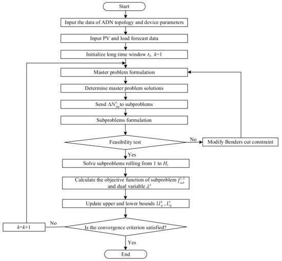
Figure 3. Flowchart of the proposed DRM strategy to solve the reactive power and voltage problem.

After collecting the parameters and forecasts in the optimization model, initialization is required to enter the Benders loop. The master problem in Equation (28) of OLTC tap position is first solved, and the lower bound $L_B^k$ of the original problem is updated according to Equation (29). Then, the result of the master problem is substituted into subproblems for feasibility test. If the OLTC tap result satisfies the constraints, the subproblems in Equation (27) are continued to be solved, and the upper bound $U_B^k$ is updated according to Equation (30). If not, the Benders cut constraint is modified to re-solve the master problem. When the difference between the upper bound and the lower bound is less than the threshold $\epsilon$ in Equation (31), the global optimal solution of the original problem has been found, otherwise the loop needs to be entered again:

$$L_B^k=c_b\Delta N_{tap}^{t_l}{}^2+{\alpha }^k$$

(29)

$$U_B^k=J_{sub}^{t_l,k}+c_b\Delta N_{tap}^{t_l}{}^2$$

(30)

$$\left|\frac{U_B^k-L_B^k}{U_B^k}\right|\le \epsilon$$

(31)

5. Results and Discussion

5.1. Simulation Results of Case 1

A modified PG&E 69-bus distribution network in Figure 4 with specific configurations in Table 2 is selected to test the optimization algorithms performance. More detailed topology information can be obtained by referring to [41]. Figure 5 shows the forecasted aggregate power profile of PV and total daily load profile. The example simulation models are implemented in the MATLAB R2018b environment, and the optimization problems are solved by a commercial solver Gurobi8.9.0 [42]. The upper and lower levels of voltage are 1.05 p.u. and 0.95 p.u. of its base value [43]. The minimum power factor of PV is set to 0.95. Moreover, the unit cost coefficient of OLTC tap is $6 [44] and the upper limit for the daily OLTC tap is set to 20 changes [45,46]. The estimated unit cost coefficient of PV active power and reactive power output are 0.8$/MW and 0.1$/MVar [47] for the economy estimation.

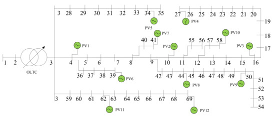
Figure 4. Modified PG&E 69-bus system with PVs.

Table 2. The basic installation parameters of OLTC and PVs.

Devices	Parameters	Values
OLTC	Tap range	−8–8
PV	Capacity	500 kWP

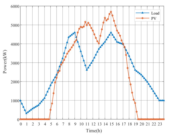
Figure 5. The aggregate daily load profile and solar power profile of Case 1.

To verify the advantages of the proposed DRM strategy, two other strategies were investigated to compare and analyze the performance in different cases, namely: single-period decoupling strategy (S1) and multi-period decoupling and non-rolling strategy (S2). The strategies are illustrated in Figure 1a,b. Table 3 further presents the differences between them in detail.

Table 3. Comparison of three voltage optimization strategies.

Characteristic	S1	S2	DRM
Decoupling of discrete/continuous device actions	√	√	√
Subdividing optimization periods	×	√	√
MPC-based rolling optimization	×	×	√

5.1.1. Optimal Results

This paper takes 11:00 and 24:00 results as examples to represent voltage deviations of the proposed DRM strategy, as shown in Figure 6. Although some nodes near the end of feeders appear overvoltage (over 1.05 p.u.) at 11:00 due to the high PV outputs, the nodal voltages return to the safe state after optimization. For the result of 24:00 without PV generation, it not only shows that each feeder has a voltage drop due to line impedance, but also illustrates the whole ADN operates within the acceptable range. The optimized overall voltage level is closer to the reference value. The voltage deviation of the Node 16 and Node 54 for a day are shown in Figure 7. The proposed DRM strategy can greatly reduce the voltage amplitudes by adjusting OLTC tap changes and PV reactive power outputs. It is worth noting that Node16, the grid-connected point of PV3, severely exceeded the upper limit at around 11:00, and the voltage drop after optimization is more obvious than that of Node 54.

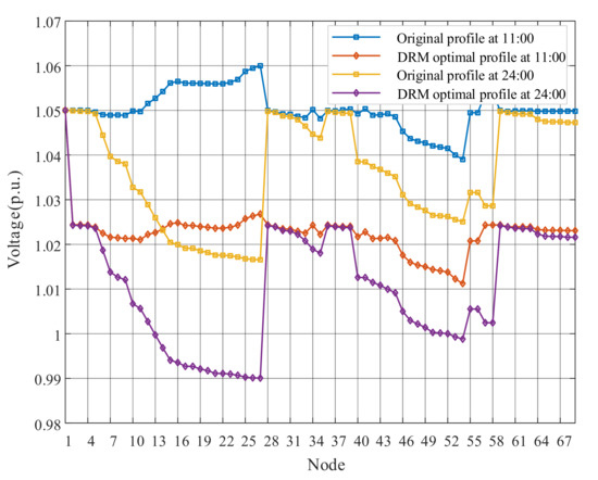
Figure 6. The nodal voltages of 11:00 and 24:00.

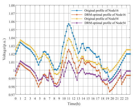
Figure 7. The daily voltages of Node16 and Node54.

Figure 8, Figure 9 and Figure 10 show the optimal operation results of OLTC tap and PV power outputs after adopting the DRM strategy. When PV generation is excessive, OLTC raises the tap to reduce the substation secondary side voltage, whereas PVs absorb reactive power to regulate voltages of the surrounding nodes. Remarkably, at around 11:00, even though the voltage has exceeded the limit, the OLTC tap is not further changed, while the active power output of PV4 in Figure 10 is reduced at noon to decrease the voltage level, due to the limited reactive power capacity. The results indicate that the adjustment of PV output can be used to address local voltage problems in feeders. However, because of the limited solar radiation in the morning from 1:00 to 6:00, PV generation is nonexistent. The OLTC tap can only be used to stabilize the voltage level. The numerical results of DRM strategy have been presented in Appendix A for this paper.

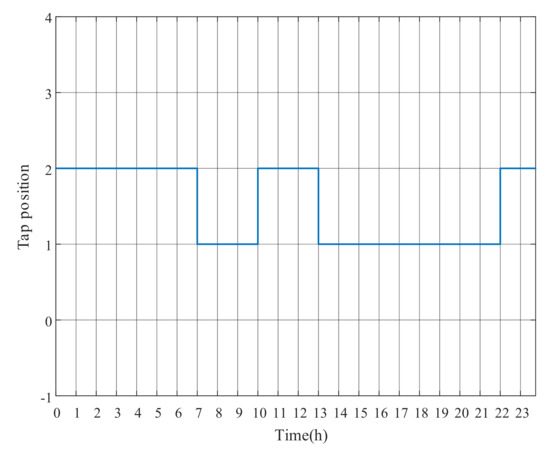
Figure 8. OLTC tap changes with DRM strategy.

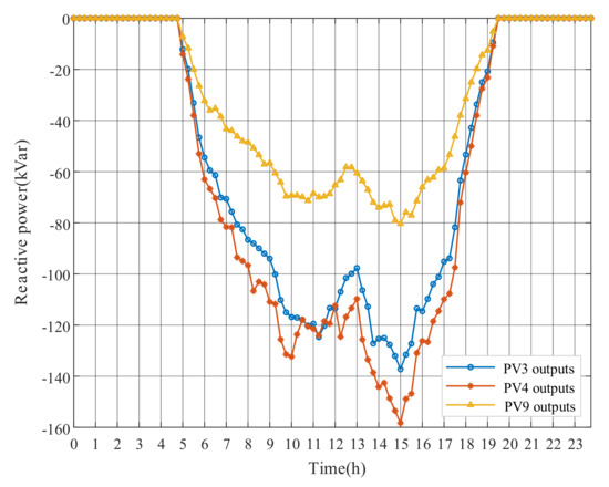
Figure 9. PV reactive power outputs with DRM strategy.

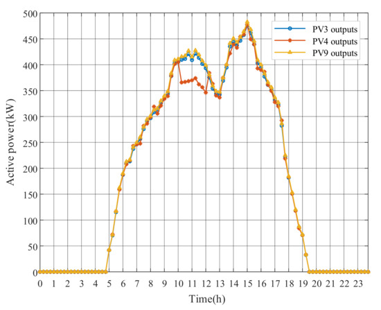
Figure 10. PV active power outputs with DRM strategy.

5.1.2. Performance Comparison

Adjustment Costs

PV reactive power outputs (for example, PV3) and OLTC tap actions of the three mentioned optimization strategies are shown in Figure 11 and Figure 12, respectively. Since the master problems of OLTC in the three strategies are set within the same long period, the results and adjustment costs of OLTC tap is the same. Table 4 shows that the adjustment costs of S1 and S2 are much higher than that of DRM strategy, which is because of the differences in PV reactive power outputs. The long-period PV forecasts applied by S1 usually present uncertainties, which leads to large changes in PV reactive power outputs of neighbored long periods, and hence the adjustment costs increase significantly. Compared with DRM, S2 lacks the rolling optimization setting of MPC algorithm based on the prediction and control horizon. The optimization function of the rolling subproblems is to gradually reduce the difference between the current state and the ideal state in the long prediction and control horizon. A series of short-period PV reactive output instructions are obtained, although only the first short-period instructions are executed. As shown in Figure 11, the PV reactive power results of several independent short-period subproblems in S2 fluctuate obviously, raising the adjustment costs of PVs, while the based-MPC DRM strategy indicates a significant reduction in cost.

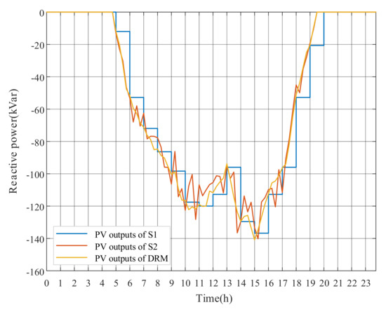
Figure 11. PV3 reactive power outputs with three strategies.

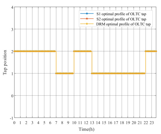
Figure 12. OLTC tap changes with three strategies.

Table 4. Adjustment costs of three strategies.

Adjustment Cost	S1	S2	DRM
OLTC	$24	$24	$24
PVs	$1.17	$1.64	$0.63
Total	$25.17	$25.64	$24.63

Voltage Deviations

In order to verify the superiority of the proposed DRM strategy in terms of voltage deviations, the voltage results at 11:00 and 24:00 from different strategies is shown in Figure 13. Three strategies can effectively reduce the voltage level, the voltage amplitude of S1 is higher than that of S2 and DRM at 11:00. The voltage results of some nodes by S2 and DRM are similar, while the voltages of the feeder from Node 13 to Node 27 by S2 are higher than the DRM strategy. The difference between the three strategies does not exist at night, because PVs do not generate electricity.

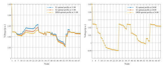
Figure 13. The nodal voltages of 11:00 and 24:00 from three strategies.

Figure 14 compares the daily voltages of Node 16 and Node 54 optimized by S1, S2 and DRM strategy from the perspective of time changes. The differences between S1 and DRM strategy are still existed, while the voltage results of S2 and DRM are similar. More accurate data are given in Table 5, which is also shows this phenomenon. For the all-day voltage deviations, compared with the original profile, the three optimization methods all achieve a voltage deviation reduction of more than 60%. The S1 voltage deviation is 0.88 p.u. more than that of the DRM due to the errors in the long-period PV forecasts, while the voltage deviation difference between S2 and DRM is 0.23 p.u.

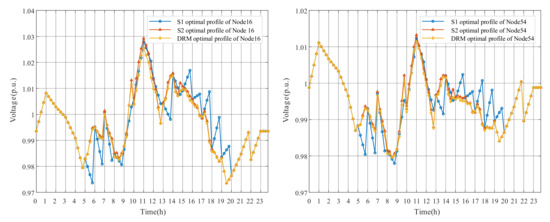
Figure 14. The daily voltages of Node16 and Node54 from three strategies.

Table 5. Voltage deviation results of three strategies.

	Original	S1	S2	DRM
All nodes at 11:00	3.4951 p.u.	1.6899 p.u.	1.6806 p.u.	1.5839 p.u.
All nodes at 24:00	2.4852 p.u.	0.9467 p.u.	0.9467 p.u.	0.9467 p.u.
Node 16 all day	1.9247 p.u.	1.0189 p.u.	1.0010 p.u.	0.9740 p.u.
Node 54 all day	1.5351 p.u.	0.6928 p.u.	0.6899 p.u.	0.6881 p.u.
All nodes all day	299.9501 p.u.	122.7256 p.u.	122.0783 p.u.	121.8496 p.u.

Active Power Losses

Table 6 shows the simulation results of the active power loss from the three strategies. Before PVs are connected to the distribution, the active power loss is as high as 4.8305 MWh a day. The distributed PV power generation can greatly reduce the network losses, only 2.0546 MWh. Due to the PV power transmission, the network loss results of the three optimization strategies are slightly higher than the original data. However, since some original nodal voltages exceed the upper limit, the voltage optimization strategy has to be implemented. Among the three strategies, S1 has the largest active power losses, because the forecast of load and PV power generation is uncertain, and the results of long-period strategy cannot achieve the dynamic optimization, resulting in a large amount of power loss. The active power loss of S2 considering different optimization periods is a little more than that of DRM strategy. The reason is that S2 is the static optimization method of each short period based on forecasts with errors, while the DRM strategy using dynamic real-time forecasts achieves the gradual approximation of the ideal value by rolling the time window.

Table 6. Active power losses from three strategies.

	No PV	Original	S1	S2	DRM
Active power losses	4.8305 MWh	2.0546 MWh	2.7143 MWh	2.6610 MWh	2.6472 MWh

Computation Time

The computation time of the three strategies is shown in Table 7. The present case only focuses on the differences in computation time caused by the optimization strategy, including modeling and solution, without considering the time spent on PV and load forecasting. Based on the 69-node distribution system configuration of Case 1 and the long period setting of S1, the 1-h daytime optimization result including OLTC tap and PV power requires 21.46 s, and the result of one day requires 5.33 min. Both S2 and the DRM strategy set the short optimization period about 15 min for PV output, and hence there are 96 changes in PV output per day. S2 takes 9.07 s to solve a short-period subproblem of PV power during the day. Since the linear sensitivity between node voltage and power is used instead of the nonlinear power flow constraints, although the optimization problems and variables have been increased by almost 4 times compared with S1, the computation time has only increased by around 2 times. The 1-h optimization requires 48.94 s, and the total computation time of one day is 11.64 min. The DRM strategy applies MPC algorithm to improve the subproblems of S2, and a short-period PV results by rolling optimization only increases by 1.36 s. The optimal results of 96 times a day takes 2.75 min longer than S2 in total. Comparing the computation time of a 1-h optimization, it can be seen that the computation time mainly depends on the number of iterations between master problems and subproblems, while the additional time required for rolling optimization of continuous PV outputs is not much. When the scale of the distribution network expands, the significant increase in nodes and discrete devices will result in more computation time.

Table 7. Computation time of three strategies.

	S1	S2	DRM
Long period (1 h) optimization	21.46 s	48.94 s	50.23 s
Short period (15 min) PV optimization	-	9.07 s	10.43 s
One day optimization	5.33 min	11.64 min	14.39 min

5.2. Simulation Results of Case 2

Compared with Case 1, Case 2 is a system configuration with uneven distribution of PVs, as shown in Figure 15. The feeder from Node 28 to Node 35 is completely passive and is not connected to any PV. The parameters of each PV source and OLTC remain unchanged, in Table 2. The forecasted aggregate power profile of PV and total daily load profile are shown in Figure 16.

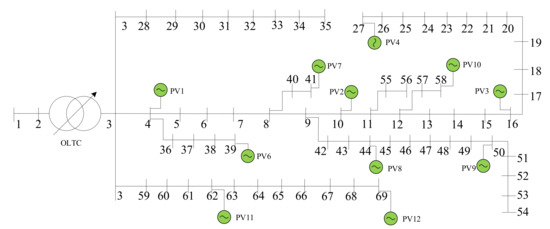
Figure 15. Modified PG&E 69-bus system with uneven PVs.

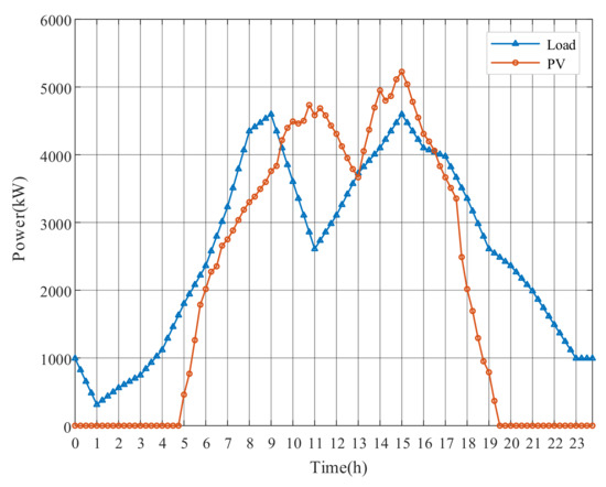
Figure 16. The aggregate daily load profile and forecasted PV power profile of Case 2.

The voltage results of all nodes at 11:00 and 24:00 are shown in Figure 17. The 11:00 voltage is significantly different from that of Case 1, and a slight overvoltage occurs in the system. In the original profile, the feeder voltage without PV connection from Node 28 to Node 35 gradually decrease due to the power loss caused by the line impedance. Compared with Case 1, the sum of original voltage deviations is smaller, and it is further reduced after optimization by DRM strategy.

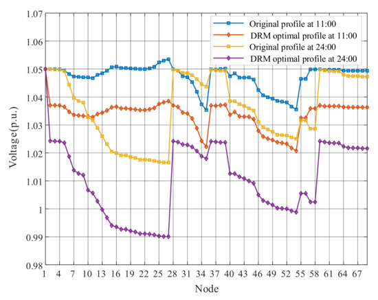
Figure 17. The nodal voltages at 11:00 and 24:00 of Case 2.

Figure 18 reflects the differences in voltage changes at Node 27 and Node 35, the ends of two feeders. The voltage of Node 27 varies considerably, which is affected by the adjustment of the PV power on the feeder between Node 4 and Node 27. The Node 35 is only affected by load fluctuations and OLTC tap adjustments, and hence the changes are small.

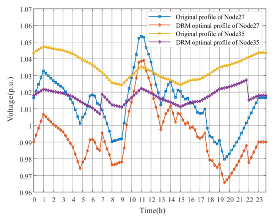
Figure 18. The daily voltages at Node27 and Node35 of Case 2.

The OLTC tap position and PV outputs of the DRM optimization strategy are shown in Figure 19, Figure 20 and Figure 21. Compared with Figure 8 of Case 1, the number of OLTC tap changes is significantly decreased, because the original node voltages of Case 2 do not excessively exceed the upper limit. The frequent OLTC tap changes are avoided due to the impact of OLTC on the substation secondary bus voltage and its higher adjustment cost. We can see that DRM strategy mainly optimizes the voltage by adjusting PV outputs. In Figure 20, PV1 and PV4 absorb a large amount of reactive power to decrease the voltage deviation. The reactive power absorption of PV9 at Node 50 is less because the end node voltage of the feeder is relatively low. From Figure 21, the PV active power outputs are still at the predicted level. It can be explained that PVs provide sufficient reactive power capacity at this time, avoiding the PV active power curtailment.

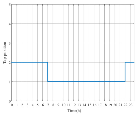
Figure 19. OLTC tap changes with DRM strategy of Case 2.

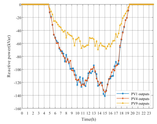
Figure 20. PV reactive power outputs with DRM strategy of Case 2.

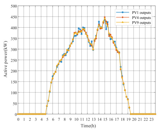
Figure 21. PV active power outputs with DRM strategy of Case 2.

6. Conclusions

In this paper, a novel DRM method is applied to the power and voltage optimization of ADN cooperating distributed PV and OLTC. According to the discrete and continuous characteristics of control variables, the proposed method utilizes a Benders decomposition algorithm to design a long-period master problem of OLTC tap and short-period subproblems of PV power outputs, achieving the decoupling of different devices actions. The different optimization time step considering the operation principles of devices not only avoids the frequent OLTC tap changes, but also further reduces voltage deviations caused by the stochastic intermittence and fluctuations of PV. The independent subproblems are then further modified into a series of rolling optimization models within long predictive and control horizons based on MPC algorithm considering the uncertainty of PV power generation and load. The rolling optimization of PV power achieves the gradual evolution of the ideal voltage in a long period without causing violent fluctuations in PV reactive power outputs, which greatly decreases adjustment costs. In the case study of the modified PG&E 69-node distribution network, the other two methods are compared to demonstrate the effectiveness and economy of DRM method. The future work would move forward to the implementation of the proposed optimization method considering the high uncertainty of renewable energy generation in large scale ADN. Besides, the impact of energy storage system on the dynamic voltage optimization is introduced. These issues would be established as subsequent research objectives.

References

- Cossent, R.; Gómez, T.; Olmos, L.; Gómez, T. Large-scale integration of renewable and distributed generation of electricity in Spain: Current situation and future needs. Energy Policy 2011, 39, 8078–8087. [Google Scholar] [CrossRef]
- Schonardie, M.F.; Martins, D.C. Application of the dq0 transformation in the three-phase grid-connected PV systems with active and reactive power control. In Proceedings of the 2008 IEEE International Conference on Sustainable Energy Technologies, Singapore, 24–27 November 2008; pp. 18–23. [Google Scholar]
- Reference Technical Rules for the Connection of Active and Passive Consumers to the HV and MV Electrical Networks of Distribution Company Issue; Italian Technical Guidelines CEI 0-16 2012-12; Comitato Elettrotecnico Italiano: Milan, Italy, 2012.
- Thomson, M.; Infield, D. Impact of widespread photovoltaics generation on distribution systems. IET Renew. Power Gener. 2007, 1, 33. [Google Scholar] [CrossRef]
- Tonkoski, R.; Lopes, L.A.C.; El-Fouly, T.H.M. Coordinated Active Power Curtailment of Grid Connected PV Inverters for Overvoltage Prevention. IEEE Trans. Sustain. Energy 2010, 2, 139–147. [Google Scholar] [CrossRef]
- Zhao, C.; Gu, C.; Li, F.; Dale, M. Understanding LV network voltage distribution- UK smart grid demonstration experience. In Proceedings of the 2015 IEEE Power & Energy Society Innovative Smart Grid Technologies Conference (ISGT), Washington, DC, USA, 18–20 February 2015; pp. 1–5. [Google Scholar]
- Dou, X.; Duan, X.; Hu, Q.; Shen, L.; Wu, Z. A nonintrusive control strategy using voltage and reactive power for distribution systems based on PV and the nine-zone diagram. Int. J. Electr. Power Energy Syst. 2019, 105, 89–97. [Google Scholar] [CrossRef]
- Zhu, Y.; Tomsovic, K. Adaptive power flow method for distribution systems with dispersed generation. IEEE Trans. Power Deliv. 2002, 17, 822–827. [Google Scholar] [CrossRef]
- Valverde, G.; Van Cutsem, T.H. Model Predictive Control of Voltages in Active Distribution Networks. IEEE Trans. Smart Grid 2013, 4, 2152–2161. [Google Scholar] [CrossRef]
- Robbins, B.A.; Hadjicostis, C.N.; Domínguez-García, A.D. A Two-Stage Distributed Architecture for Voltage Control in Power Distribution Systems. IEEE Trans. Power Syst. 2012, 28, 1470–1482. [Google Scholar] [CrossRef]
- Sulc, P.; Backhaus, S.; Chertkov, M. Optimal Distributed Control of Reactive Power via the Alternating Direction Method of Multipliers. IEEE Trans. Energy Convers. 2014, 29, 968–977. [Google Scholar] [CrossRef]
- Calderaro, V.; Galdi, V.; Massa, G.; Piccolo, A. Distributed generation management: An optimal sensitivity approach for decentralized power control. In Proceedings of the 2012 3rd IEEE PES Innovative Smart Grid Technologies Europe (ISGT Europe), Berlin, Germany, 14–17 October 2012; pp. 1–8. [Google Scholar] [CrossRef]
- Calderaro, V.; Conio, G.; Galdi, V.; Massa, G.; Piccolo, A. Optimal Decentralized Voltage Control for Distribution Systems with Inverter-Based Distributed Generators. IEEE Trans. Power Syst. 2013, 29, 230–241. [Google Scholar] [CrossRef]
- Turitsyn, K.; Sulc, P.; Backhaus, S.; Chertkov, M. Options for Control of Reactive Power by Distributed Photovoltaic Generators. Proc. IEEE 2011, 99, 1063–1073. [Google Scholar] [CrossRef]
- Cai, Y.; Tang, W.; Li, L.; Zhang, B.; Zhang, L.; Wang, Y. Multi-mode adaptive local reactive power control method based on PV inverters in low voltage distribution networks. IET Gener. Transm. Distrib. 2020, 14, 542–551. [Google Scholar] [CrossRef]
- Molina-Garcia, A.; Mastromauro, R.A.; Garcia-Sanchez, T.; Pugliese, S.; Liserre, M.; Stasi, S. Reactive Power Flow Control for PV Inverters Voltage Support in LV Distribution Networks. IEEE Trans. Smart Grid 2016, 8, 447–456. [Google Scholar] [CrossRef]
- Dickert, J.; Domagk, M.; Schegner, P. Benchmark low voltage distribution networks based on cluster analysis of actual grid properties. In Proceedings of the 2013 IEEE Grenoble Conference, Grenoble, France, 16–20 June 2013; pp. 1–6. [Google Scholar]
- Kabir, M.N.; Mishra, Y.; Ledwich, G.; Dong, Z.Y.; Wong, K.P. Coordinated Control of Grid-Connected Photovoltaic Reactive Power and Battery Energy Storage Systems to Improve the Voltage Profile of a Residential Distribution Feeder. IEEE Trans. Ind. Inform. 2014, 10, 967–977. [Google Scholar] [CrossRef]
- Mumtaz, F.; Syed, M.H.; Al Hosani, M.; Zeineldin, H.H. A Novel Approach to Solve Power Flow for Islanded Microgrids Using Modified Newton Raphson with Droop Control of DG. IEEE Trans. Sustain. Energy 2015, 7, 493–503. [Google Scholar] [CrossRef]
- Biserica, M.; Berseneff, B.; Besanger, Y.; Kieny, C. Upgraded Coordinated Voltage Control for Distribution Systems. In Proceedings of the IEEE Trondheim PowerTech, Trondheim, Norway, 19–23 June 2011; pp. 1–6. [Google Scholar] [CrossRef]
- Zhang, B.; Lam, A.Y.S.; Dominguez-Garcia, A.D.; Tse, D. An Optimal and Distributed Method for Voltage Regulation in Power Distribution Systems. IEEE Trans. Power Syst. 2014, 30, 1714–1726. [Google Scholar] [CrossRef]
- Ahmed, M.; Bhattarai, R.; Hossain, S.J.; Abdelrazek, S.; Kamalasadan, S. Coordinated voltage control strategy for voltage regulators and voltage source converters integrated distribution system. In Proceedings of the 2017 IEEE Industry Applications Society Annual Meeting, Harbor, MD, USA, 14–17 January 2017; pp. 1–8. [Google Scholar]
- Castillo, A.; Gayme, D.F. Profit maximizing storage allocation in power grids. In Proceedings of the 52nd IEEE Conference on Decision and Control, Florence, Italy, 10–13 December 2013; pp. 429–435. [Google Scholar]
- Bose, S.; Gayme, D.F.; Topcu, U.; Chandy, K.M.; Bose, S. Optimal placement of energy storage in the grid. In Proceedings of the 2012 IEEE 51st IEEE Conference on Decision and Control (CDC), Maui, HI, USA, 10–13 December 2012; pp. 5605–5612. [Google Scholar]
- Nasrolahpour, E.; Kazempour, S.; Zareipour, H.; Rosehart, W.D. Strategic Sizing of Energy Storage Facilities in Electricity Markets. IEEE Trans. Sustain. Energy 2016, 7, 1462–1472. [Google Scholar] [CrossRef]
- Nick, M.; Cherkaoui, R.; Paolone, M. Optimal siting and sizing of distributed energy storage systems via alternating direction method of multipliers. Int. J. Electr. Power Energy Syst. 2015, 72, 33–39. [Google Scholar] [CrossRef]
- Yan, W.; Yu, J.; Yu, D.; Bhattarai, K. A new optimal reactive power flow model in rectangular form and its solution by predictor corrector primal dual interior point method. IEEE Trans. Power Syst. 2006, 21, 61–67. [Google Scholar] [CrossRef]
- Esmin, A.; Lambert-Torres, G.; De Souza, A.Z. A hybrid particle swarm optimization applied to loss power minimization. IEEE Trans. Power Syst. 2005, 20, 859–866. [Google Scholar] [CrossRef]
- Li, Y.; Li, M.; Wu, Q. Optimal reactive power dispatch with wind power integrated using group search optimizer with intraspecific competition and lévy walk. J. Mod. Power Syst. Clean Energy 2014, 2, 308–318. [Google Scholar] [CrossRef]
- Farivar, M.; Low, S.H. Branch Flow Model: Relaxations and Convexification—Part I. IEEE Trans. Power Syst. 2013, 28, 2554–2564. [Google Scholar] [CrossRef]
- Wang, C.; Xiang, L.; Deng, Z.; Liang, Z. Reactive Power Optimization Dispatch Strategy in Distribution Network with Distributed Generators. J. Eng. 2017, 2017, 1418–1422. [Google Scholar] [CrossRef]
- Chen, L.; Deng, Z.; Xu, X. Two-Stage Dynamic Reactive Power Dispatch Strategy in Distribution Network Considering the Reactive Power Regulation of Distributed Generations. IEEE Trans. Power Syst. 2018, 34, 1021–1032. [Google Scholar] [CrossRef]
- Maciejowski, J.M. Predictive Control with Constraints; Prentice-Hall: Englewood Cliffs, NJ, USA, 2002. [Google Scholar]
- Glavic, M.; Hajian, M.; Rosehart, W.; Van Cutsem, T.H. Receding-Horizon Multi-Step Optimization to Correct Nonviable or Unstable Transmission Voltages. IEEE Trans. Power Syst. 2011, 26, 1641–1650. [Google Scholar] [CrossRef]
- Fortenbacher, P.; Ulbig, A.; Andersson, G. Optimal Placement and Sizing of Distributed Battery Storage in Low Voltage Grids Using Receding Horizon Control Strategies. IEEE Trans. Power Syst. 2017, 33, 2383–2394. [Google Scholar] [CrossRef]
- Hug-Glanzmann, G. Coordination of intermittent generation with storage, demand control and conventional energy sources. In Proceedings of the 2010 IREP Symposium Bulk Power System Dynamics and Control—VIII (IREP), Rio de Janeiro, Brazil, 1–6 August 2010; pp. 1–7. [Google Scholar] [CrossRef]
- Bolognani, S.; Zampieri, S. On the Existence and Linear Approximation of the Power Flow Solution in Power Distribution Networks. IEEE Trans. Power Syst. 2015, 31, 163–172. [Google Scholar] [CrossRef]
- Yang, Z.; Wu, R.; Yang, J.; Long, K.; You, P. Economical Operation of Microgrid with Various Devices Via Distributed Optimization. IEEE Trans. Smart Grid 2015, 7, 1–11. [Google Scholar] [CrossRef]
- Nick, M.; Cherkaoui, R.; Paolone, M. Optimal Allocation of Dispersed Energy Storage Systems in Active Distribution Networks for Energy Balance and Grid Support. IEEE Trans. Power Syst. 2014, 29, 2300–2310. [Google Scholar] [CrossRef]
- Niknam, T.; Zare, M.; Aghaei, J. Scenario-Based Multiobjective Volt/Var Control in Distribution Networks Including Renewable Energy Sources. IEEE Trans. Power Deliv. 2012, 27, 2004–2019. [Google Scholar] [CrossRef]
- Baran, M.; Wu, F. Optimal capacitor placement on radial distribution systems. IEEE Trans. Power Deliv. 1989, 4, 725–734. [Google Scholar] [CrossRef]
- GUROBI. Available online: http://www.gurobi.com (accessed on 22 February 2018).
- National Bureau of Quality Supervision. Inspection and Quarantine and National Standardization Management Committee. National Standard of the People’s Republic of China GB/T12325-2008 Power Quality and Voltage Deviation; National Bureau of Quality Supervision: Beijing, China, 2008.
- Zhang, Y.-J.; Ren, Z. Optimal Reactive Power Dispatch Considering Costs of Adjusting the Control Devices. IEEE Trans. Power Syst. 2005, 20, 1349–1356. [Google Scholar] [CrossRef]
- Wong, T. Co-ordination of transformer tap and capacitor operation for reactive power voltage control in a distribution primary substation. In Proceedings of the APSCOM 2000—5th International Conference on Advances in Power System Control, Operation and Management, Hong Kong, China, 30 October–1 November 2000; Volume 2000, pp. 479–485. [Google Scholar]
- Sun, C.; Xu, J.; Cai, B.; Yang, Z.; Li, X. Research on efficiency increase of the automatic voltage control system in Shanghai urban power grid. In Proceedings of the 8th Renewable Power Generation Conference (RPG 2019), Shanghai, China, 24–25 October 2019; pp. 1–6. [Google Scholar]
- Khan, I.; Li, Z.; Xu, Y.; Gu, W. Distributed control algorithm for optimal reactive power control in power grids. Int. J. Electr. Power Energy Syst. 2016, 83, 505–513. [Google Scholar] [CrossRef]
Publisher’s Note: MDPI stays neutral with regard to jurisdictional claims in published maps and institutional affiliations. |
© 2020 by the authors. Licensee MDPI, Basel, Switzerland. This article is an open access article distributed under the terms and conditions of the Creative Commons Attribution (CC BY) license (http://creativecommons.org/licenses/by/4.0/).