Abstract
In this paper, the Greitzer surge model was systematically analysed with the model compressor duct length Lc as the tuning parameter. The surge phenomenon is known to induce a serious risk to centrifugal compressor operation. The two-dimensional Greitzer model is a well-established way of modelling this dangerous instability, but the determination and changes of the model parameters are still being discussed. In this paper an automated procedure determines the Lc value providing the best fit with the experimental data has been presented. The algorithm was tested on five valve positions and revealed that the best fit was obtained for different Lc values following a linear trend against the mass flow rate. The study has also shown that the Greitzer model has two solutions for a given pressure oscillation amplitude: one similar to the deep surge (low Lc) and one similar to the mild surge (low Lc). This suggests that this model can be used to simulate both types of the phenomenon known from the experimental analyses. The study proposes the dimensionless average pressure as the parameter allowing to distinguish which surge cycle was observed at a given instance. Past papers were analysed to observe the surge type that appeared in different experiments. It was found that most researchers obtained low Lc surge. The results show that both deep and mild surge could be simulated with the Greitzer model. It also revealed that the Lc should not be treated as a constant value for a given machine and that it changes with the mass flow rate.
1. Introduction
The operating range of radial compressors is limited due to the flow instabilities occurring at low mass flow rate conditions. The most dangerous flow phenomenon is the surge connected with strong pressure and mass flow oscillations [1]. This phenomenon results in reduced performance and high noise levels, but also generates heavy loads on the blades and shaft, which can damage the machine [2]. In order to avoid the surge, a safety margin is set and the compressor operates at higher mass flow rates. This limitation of the operating range is highly undesired in some applications. To the contrary, a small surge margin is very risky. Thus, understanding and providing effective protection against surge became an important issue for researchers.
The ability to model the surge phenomenon is an important direction of studies pursued by numerous researchers. The most commonly used mathematical model that describes surge is the Greitzer model [3] developed in 1976. It was tested experimentally for the first time in the same year [4]. Originally, this model was developed for axial compressors but it can also be used successfully in centrifugal compressors, as proven in numerous studies [5,6,7,8]. Many confirmed and tested anti-surge systems [9,10,11,12] or control algorithms for anti-surge systems [13,14] originate from the Greitzer model. Some researchers also introduced modifications to the model to adjust it to a particular application. For example, pipeline acoustics was added to the model by Yoon et al. [15,16] or by van Helvoirt and de Jager [17].
Modelling a compressor with the use of the Greitzer or Greitzer-based mathematical models is always very challenging when compared to experimental data. The original Greitzer model is four-dimensional. Its modifications could either increase this number slightly [17,18] or decrease it to only two dimensions [7,19,20]. One could expect that such models provide a much smoother response than the measured data affected by numerous higher-order phenomena and noise. Additionally, in order to develop an effective and reliable way of suppressing or avoiding surge, it is very important to model the compressor precisely during the surge.
The Greitzer model is also dependent on a set of parameters that need to be defined. Some of them have a clear physical aspect like the plenum volume, the speed of sound, the frequency of the Helmholtz resonator, and the time needed to develop a full rotating stall pattern. Others could be interpreted in many different ways: the compressor duct area, the compressor duct length, the valve duct area and the valve duct length. In most papers, these parameters were selected based on the impeller geometry or according to best fit with the experimental data [16,17,18,21,22,23]. The model is usually tested at one valve position. It is commonly believed that compressor dynamics, and hence the Greitzer model parameter Lc, is constant for all compressor mass flow rates.
In this paper, compressor operation during surge has been modelled at multiple operational points using the Greitzer model. For each situation, the optimal Lc value was chosen to provide the best agreement with the experimental data. The aim was to ascertain whether the function Lc = f() is indeed constant.
2. Method
2.1. Experimental Rig and Measurements
A single-stage centrifugal blower DP1.12 was modelled in this paper. It was designed and constructed by Magiera [24] and then modified for surge investigation. Its further description can be found in [24]. Figure 1 presents its cross-section along with the main dimensions.
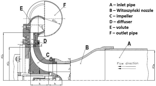
Figure 1.
Cross-section of DP1.12 blower.
The flow entered the blower through an inlet pipe (A) of diameter and then accelerated via a Witoszyński nozzle [25] (B). The impeller (C) hub diameter was equal to and the inlet blade span was equal to . At the outlet, the diameter and blade span were equal to and respectively. The rotor had 23 blades. The inlet area of the passage cross-section equalled and at the outlet . Upon exit, the rotor flow entered the vaneless diffuser (D) with an outlet diameter . Downstream flow was gathered by volute (E) of radius , which gradually increased streamwise from the volute tongue gap of 5 mm towards the outlet pipe with a diameter equal to . The outlet pipe had two straight sections, 250 and 3750 mm long, and one elbow between them. At its end, this reached a throttling pipe.
The machine was driven by an asynchronous AC motor. Rotational speed during measurements was with nominal mass flow rate and pressure ratio . Rotational speed yielded the impeller tip speed equal to .
Static pressure measurements were conducted with Kulite pressure transducers located at the inlet before the Witoszyński nozzle, and at the volute outlet. This allowed to calculate the pressure rise of the compressor. The sampling frequency was 100 kHz and the measured signal was 20.97 s long, which corresponds to over 2000 rotor revolutions.
2.2. Compressor Performance Curve
The most common method of compressor performance curve approximation used in the literature is the third order polynomial [5,16,26,27,28] presented in Figure 2 and Equation (1).
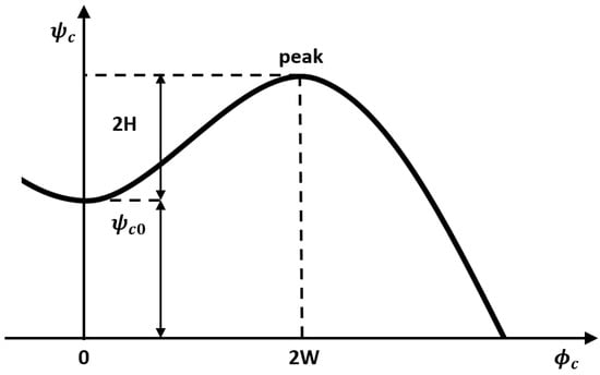
Figure 2.
Third order polynomial compressor performance curve approximation [29].
Both functions provided good fit in the region close to the points used as reference. Both could, therefore, be used for a narrow range of the mass flow rates. For a wider range, a new formula is proposed based on the fourth order polynomial. It was derived from the five conditions presented in Figure 3 and in Equations (2)–(6).
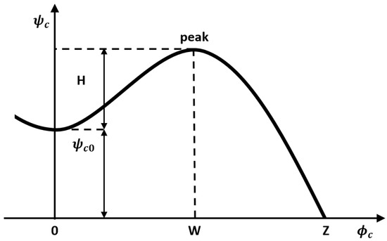
Figure 3.
Fourth order polynomial compressor performance curve approximation.
The values of W, H and were chosen by the Root Mean Square (RMS) method to provide the closest fit to the experimental results. The fit, however, was significantly far from the measured points at the highest and lowest mass flow rates. Therefore, two different third order polynomials were calculated. The first was generated by the RMS method based on “stable operation points”, while the second was generated by the same method based on “unstable operation points” (see Figure 4). All points correspond to the average value of the mass flow rate and pressure rise obtained throughout the measurement.
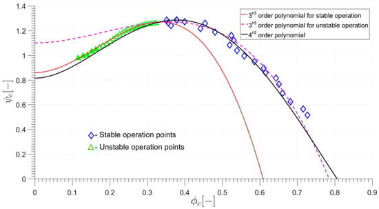
Figure 4.
Analysed compressor performance curves.
The polynomial is defined by Equation (7):
The compressor performance curves obtained by all three methods are presented in Figure 4 with both stable and unstable operation points from the experiment. One can clearly see that the fourth order polynomial provided a significantly better fit and, hence, it was used in further study. The reason why the determined performance curve in the unstable region lies slightly beneath the measured pressure is that average pressure of the surge oscillation is always higher than the set operational point, which is shown in Figure 8. Additionally, the shape of the curve has been optimised to minimise the differences between measurements and simulation.
This study was conducted at the five most unstable points, which are marked as filled triangles in Figure 4. All unstable points are denoted with triangles. Positioning of those points is a matter of discussion [29] as the machine operates along the open cycle in this regime [2]. In this plot their position is determined by the average value of pressure oscillations and by the mass flow calculated from the measured dynamic pressure profile in the outlet pipe.
2.3. Compressor Numerical Model
In this study, the two-equation Greitzer model [3,4] was used, proving to be a good choice for the centrifugal compressor [2]:
where and are respectively dimensionless mass flow and pressure, defined as:
where is gas density. The subscripts c and t correspond to the model compressor and throttle duct respectively. The values of and being a solution of the Greitzer equations define the compressor operation. Time is scaled with the Helmholtz frequency :
Parameter B is named as the Greitzer stability parameter. Its value defines system stability.
The speed of sound in normal operation conditions is constant and equal to . Blade tip speed was equal to . Geometrical parameters: plenum volume , compressor duct area and compressor duct length can be obtained from the compressor geometry. Plenum volume is equal to the sum of all element volumes from the diffuser outlet to the receiver or throttle valve (in this study ). The compressor area can be connected with the rotor outlet area or the outlet area of the single passage. In this analysis, the first possibility was chosen (). The choice of is also often connected with the compressor diameter or the length of a single passage. Nevertheless, the last two values are often selected based on the compressor dynamics rather than its physical features. Model compressor length is commonly used as a tuning parameter [23,30], which was firstly done by Badmus et al. [31] in the study of the axial compressor.
2.4. Description of the Algorithm
In this paper, the same modelling algorithm was used for all five operational points. It is visualised as a block diagram in Figure 5. Pressure signals gathered from the experiment were transformed into dimensionless mass flow and pressure rise. Based on this data and by using the Fast Fourier Transform (FFT) algorithm, the amplitude and frequency of pressure oscillations were gathered.
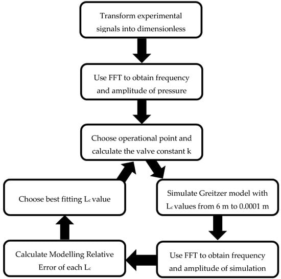
Figure 5.
Modelling algorithm.
The compressor operational point was determined based on the average values of measured pressure and mass flow rate. This point is visually defined as the crossing of two lines: compressor and throttle performance curves. Therefore, if the first curve and the operational point is defined it is possible to calculate the throttle constant and, subsequently, the throttle characteristics were calculated from Equation (14).
When the operational point is defined by the compressor performance curve and the throttle resistance curve, the Greitzer model can be implemented. All parameters, except Lc, were designated from the compressor geometry and rotational speed as described before. A wide spectrum of Lc values was simulated to investigate its effect on the simulated surge amplitude and frequency. At this point, the optimal value of Lc could be selected.
Values of Lc from 6 m to 0.01 m with a step equal to 0.001 m and from Lc from 0.01 to 0.0001 m with a step equal to 0.0001 m were analysed. This spectrum was sufficiently wide to detect a suitable Lc value and to inspect the influence of this parameter on the modelled surge phenomenon. All obtained signals were analysed with the MatLab build-in FFT algorithm. From the signal frequency spectrum, the amplitude and frequency values of the highest peak were automatically registered. To determine the most suitable Lc value The Modelling Relative Error (MRE) was introduced. It was calculated as the square root of the sum of squares of relative errors of the amplitude and the frequency for each simulation. The MRE method of calculation is presented in Figure 6. The simulation with the smallest value of MRE was considered as the best fit to the experimental data. It has to be outlined that the MRE does not represent an error in classic understanding (like measurement error or numerical error). MRE describes the relative difference in two most crucial parameters observed in the experiment and obtained in the model. It is expected that a model with two degrees of freedom and including numerous simplifications [19] should indeed differ in outcome from the experimental observation. Nevertheless, the smaller MRE, the better fit between the model and experimental observation.
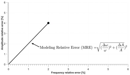
Figure 6.
Modelling relative error calculation method.
After performing these operations, a new operational point was chosen and the algorithm was run again. The described modelling procedure was implemented and calculated in MatLab.
3. Results
In Figure 7, the amplitude of pressure signal oscillations from simulations in the function of the Lc parameter are presented. It is noted that in all operational points oscillation amplitude grew until it achieved a maximum value and then decreased. Lc values, at which simulation amplitude achieved values near 0, were different for all operational points, which was caused by the different critical value of stability parameter B. As expected, the unstable region was wider for smaller average mass flows. The maximum value of amplitude remained almost the same for all operational points while the value of Lc during this time was decreasing with the rise of the mass flow.
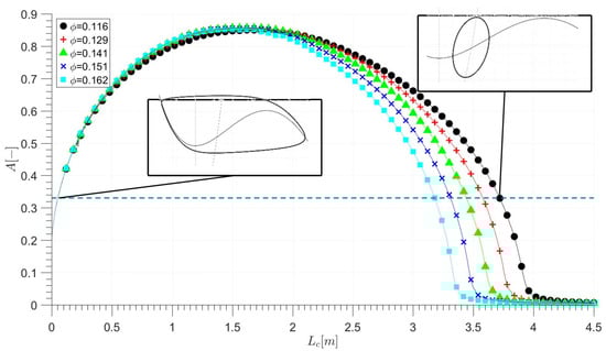
Figure 7.
Pressure oscillations amplitude for different operational points and Lc parameter value.
The dashed horizontal line corresponds to one of the amplitudes registered in the experiment. One can observe that there are always two values of the Lc parameter to which the amplitude is equal. This is a very important conclusion showing that there are always two solutions of the Greitzer model that correspond to a registered amplitude. Each of them would, however, be characterised by a different frequency and shape of oscillations.
Figure 8 presents simulated surge limit cycles obtained with two different values of Lc parameter for mass flow c = 0.116. Despite the fact that values of pressure amplitudes are the same, it is evident that cycles represent different phenomena. The black curve with circles obtained with a lower Lc value shows a cycle that has a shape similar to typical deep surge cycles [2]. The blue line with diamonds shows elliptic oscillations typical for small values of B and could be more associated to mild surge. In the middle of Figure 8, the black circle and blue diamond, which are empty inside, represent the average mean pressure and mass flow oscillation, thus the centre of oscillations. As one may notice, those values are in both cases higher than the set operational point. This means that the common practice of using the average pressure value of the unstable signal for compressor performance curve determination is inappropriate.
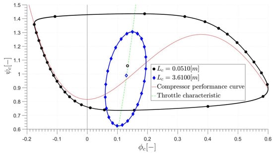
Figure 8.
Simulated surge limit cycles using two different values of Lc parameter for mass flow = 0.116.
It is not clear which cycle would appear in a given machine. This could be easily confirmed by analysing the mass flow rate oscillations or the average value of the oscillation. In this study, the difference between the amplitude of the measured pressure signal and the simulation using higher values of Lc (right-hand side) was smaller than 1% in all investigated operational points.
Figure 9 presents the frequency of pressure signal oscillations obtained in simulations in the function of Lc. It is noted that in all operational points, oscillations frequency decreased with the increase of the Lc parameter value. For low values of Lc, the frequency had very high values reaching 700 rad/s and the slope of the curve was very steep (the Y axis was limited to 200 rad/s to facilitate reading of the chart). Valve position had a minor impact on pressure oscillations frequency. On the left-hand side of the figure, it is clear that for higher mass flows oscillations were slightly more frequent, while after reaching approximately Lc = 1.5 m, the dependency reversed and lower mass flows oscillated slightly more frequently. The dashed horizontal line corresponds to one of the frequencies registered during the experiment. In opposition to the amplitude, there was only one value of the Lc parameter at which the simulation had the same frequency as the real pressure signal.
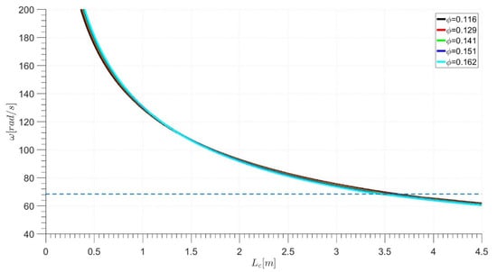
Figure 9.
Pressure oscillations frequency for different operational points and Lc parameter value.
Figure 10 presents modelling, amplitude and frequency relative error in a function of the valve position and resulting average dimensionless mass flow rate. One can notice the general trend whereby minimal MRE rises with the increase of the mass flow. This dependency is expected because the oscillations in the machine are becoming weaker with higher mass flow rate and the surge model becomes less successful in reproducing the signal. Another important observation is that the impact of amplitude relative error on MRE was negligible, while frequency relative error was almost equal to MRE. This showed that it was much more difficult for the algorithm to find a close frequency than the amplitude. Nevertheless, the algorithm allowed to find a Greitzer model for each case that reconstructed the system’s behaviour with an error not higher than 3.5%.
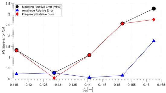
Figure 10.
Modelling, amplitude and frequency relative error in dimensionless mass flow function.
Figure 11 shows an example of the result of such a fit. The graph on the left-hand side shows the comparison between the experimental signal and the simulated Greitzer model. The plot on the right-hand side shows the frequency spectrum obtained with the Fourier transform from both signals. It is evident that the pressure signals are slightly different due to the higher order components and noise in the experimental signal. This is a normal difference observed in the Greitzer model. Both plots, however, show very similar features of the main harmonic component—the surge.
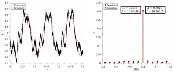
Figure 11.
Comparison between experimental signal and simulation results (left) and frequency spectrum of experimental signal and simulation results (right) for = 0.116.
Figure 12 presents the obtained Lc parameter values at different operational points. One can observe that this value decreased slightly with mass flow rate. Approximation with the first order polynomial gave a satisfactory value coefficient of determination equal to 0.99, which proves very good agreement between the results and the linear approximation.
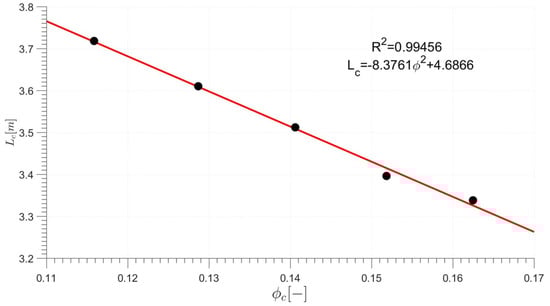
Figure 12.
Parameter Lc value as function of mass flow with linear approximation.
4. Discussion
4.1. Is Lc Constant or Changing?
In the literature, few papers present results of compressor modelling in more than three operational points. Many studies consider one valve position [12,22,23] where one constant value of Lc is used. In a study conducted by van Helvoirt and de Jager [17], the operational point change was realised via rotational speed change rather than throttling. Throttling was used by Yoon et al. [16]. The authors used a constant value of Lc.
Ng et al. included the influence of Lc as part of a wider theoretical sensitivity study using the Taguchi method [32]. The results of this study have shown that the Lc parameter has a much weaker influence on the system’s dynamics and stability compared to other considered parameters: B, G, K.
Additionally, in [22] the authors claimed that Lc has a small effect on surge amplitude and frequency, while in the present paper it was proven that it has a significant impact on them. This discrepancy might be caused by the sizeable disproportion of plenum volumes in both papers. Here, plenum was relatively small (), while in [22] plenum was substantially larger () and, thus, the dynamical response of the compressor may be having a much smaller influence on the system.
In this paper, the influence of the Lc parameter on the Greitzer model was analysed alone in a wide spectrum and compared to the experimental data. The compressor surge was modelled in five operational points with the use of the Greitzer model. The MRE (Modelling Relative Error) was proposed as a parameter for assessing the model fit to the experimental data. The graphical interpretation of this parameter is presented in Figure 6. The Lc value was chosen for each valve position in such a way that the MRE value was minimal. The obtained MRE values presented in Figure 10 did not exceed 7%, which was a satisfactory result. One needs to remember that all attempts to simulate the real system with an enormous number of degrees of freedom is simulated with a two-dimensional model. Frequency relative error was the main component of the observed error, while amplitude relative error was kept on a much lower level. This was also influenced to some extent by the resolution of the FFT algorithm in the frequency domain.
In [22], the authors claimed that Lc might not be the best choice for this purpose. It was claimed that the same effect can be obtained by changing the compressor performance curve valley point or the Ac value. The static compressor performance curve, however, is unique for a given machine, while the discussion about defining a dynamical component of the performance curve is still ongoing. One of the ways to include the dynamic performance curve component is to use another Greitzer model equation that includes the influence of the relaxation time [6]. From a mathematical point of view, the change of Lc can be compensated with an opposite change of Ac. The second parameter, however, is easy to be associated with the geometry of the compressor. In the literature, it is widely considered to be an area of the diffuser inlet or the impeller eye [16]. Therefore, based on the present study, one can claim that the Lc is a good tuning parameter in the process of compressor surge modelling.
In fact, Lc could also vary with the valve position. Figure 12 shows that Lc values changed linearly with the mass flow rate. High R2 confirmed that this trend is strong. We believe that this tendency was not presented in the literature because the number of studies using a large number of valve positions was limited. This observation allows to predict compressor behaviour during surge at any operational point even if only a few Lc values are known and the linear function is described based on them. Measuring pressure signals in mild surge can result in the prediction of the surge cycle in dangerous conditions of deep surge.
4.2. Two Types of Surge
Figure 7 shows that there are two points at which the Greitzer model’s amplitude fits to the experimental data. Both surge cycles, however, are significantly different (Figure 8) and have different frequencies (Figure 9). The cycle observed at low Lc (known henceforth as “low Lc surge”) resembles much wider mass flow oscillations and much higher oscillation frequency. The oscillation cycle is close to the shape of the performance curve. It could be associated to the deep surge widely observed in the literature [17,22,33]. The cycle obtained at high value of L (known henceforth as “high Lc surge”) has a much higher frequency, but smaller amplitude of mass flow rate. The shape of a cycle in this case is elliptical. One could associate this phenomenon with the mild surge widely described in the literature [2,19].
In this study, the high Lc surge fit better to the experiment. We conducted a literature review to investigate which cycles have been observed in other studies. Table 1 presents the data gathered from the relevant papers. The first conclusion is that this information cannot be directly derived from the presented data. Neither model parameters (for example, Ac, Vp) nor compressor working conditions (for example, nominal rotational speed or nominal power) could be treated as unambiguous indicators of the surge cycle type.

Table 1.
Summary of data from articles concerning surge modelling in centrifugal compressors.
Another problem lies in the number of presented compressor and corresponding Greitzer model parameters. For example, the mass flow rate oscillations could be used as an easy distinguishing factor. Dynamic mass flow rate measurements are, however, uncertain and difficult to perform. Not all studies included the information whether the reverse flow was observed. Therefore, it is most convenient to have a parameter based solely on pressure measurement and the performance curve, both of which are usually presented. In Figure 8, one can observe a different position of the average pressure compared to the performance curve. Low Lc surge is characterised by the average value located somewhere close to the middle between the local minimum (valley point) and maximum (peak point) of the performance curve as it follows its shape. The high Lc surge cycle is more local and the average pressure would be close to the intersection of the resistance and performance curves, which could be possibly lower or higher than the mid-way between the minimum and maximum of the performance curve. This leads to the introduction of the dimensionless average pressure as a distinguishing factor. Its definition is presented below:
and values are taken from the compressor performance curve. represents the pressure at the curve peak (close to the nominal point), while represents the pressure at the curve valley (for zero mass flow rate). stands for the mean value of the pressure oscillations of the observed surge cycle calculated peak to peak. The values of represent the dimensionless position of the pressure average value between the peak and valley of the performance curve. Values in the ranges of 0–0.4 and 0.6–1 mean that average pressure oscillations are close to the peak or valley point and, thus, it is highly probable that high Lc surge is present (that could be treated as mild surge). Values in the range of 0.4–0.6 mean that the average pressure is close to the mid-way between performance curve peak and valley. This might suggest low Lc surge (that could be treated as deep surge). One needs to keep in mind that it might be theoretically possible to have high Lc surge with close to 0.5 if the intersection between the performance and resistance curves is contained in this region. Therefore, it is always beneficial to know whether the reversed flow was observed. Conversely, one might expect that the reverse flow could be possible for high Lc surge with very small values of .
Table 1 presents the summary of calculations of for published papers. Data for source [23] were calculated from dimensionless pressure values. In the case of [33], the values of the valley and peak pressure of the modelled compressor performance curve were not provided and, thus, were approximated from similar rotational speed curves presented in this paper. It is notable that in all three papers where the authors state that the reverse flow took place, the value of was in the range of 0.4–0.6. It actually belonged to this range in all studies except this paper and [16]. In the study conducted by Yoon et al., the value was significantly smaller. Therefore, it is likely that in this research high Lc surge was observed (that could be treated as mild surge). The values of obtained in the current study are also not in the range of 0.4–0.6 for all analysed valve positions. This suggested that mild surge was observed and that the reverse flow did not happen.
Based on the above discussion, the newly introduced parameter is very helpful in determining which cycle was observed in a given study. close to 0 or 1 implies that high Lc surge was observed (that could be treated as mild surge). In the range between approximately 0.4–0.6, the information concerning the occurrence of reverse flow is necessary. If reverse flow is observed, so is low Lc surge (that could be treated as deep surge). If reverse flow is not observed, high Lc surge is present (that could be treated as mild surge).
5. Conclusions
In this paper, a systematic approach to compressor modelling has been presented. A small power compressor has been modelled in five unstable operating points using the Greitzer model and compared to experimental data. The conducted procedure allowed for the fit of experimental data with a modelling relative error (MRE) not higher than 3.5%. The results lead to the conclusion that the Greitzer model parameter Lc could be a good candidate as the tuning parameter of the model. Moreover, the Lc changed its value according to a change in valve position and followed a linear trend.
It was observed that there are two values of this parameter in which pressure oscillations have the same amplitude, but that the character of those oscillations, as well as the oscillation frequency, is significantly different. This means that the Greitzer model can reproduce two types of surge:
- High Lc surge (that could be treated as mild surge) has a much higher frequency but smaller amplitude of mass flow rate. The shape of a cycle in this case is elliptical.
- Low Lc surge (that could be treated as deep surge) resembles much wider mass flow oscillations and much higher oscillation frequency. The oscillation cycle is close to the shape of the performance curve.
The parameter has been introduced to determine the surge cycle type based on pressure readings and the performance curve. close to 0 or 1 implies that high Lc surge was observed (that could be treated as mild surge). In the range between approximately 0.4–0.6, information concerning reverse flow occurrence is necessary. If reverse flow is observed the system encounters the low Lc surge (that could be treated as deep surge). If reverse flow is not observed, high Lc surge is present (that could be treated as mild surge).
Author Contributions
Conceptualization, F.G. and G.L.; Funding acquisition, G.L.; Investigation, F.G.; Methodology, F.G. and G.L.; Software, F.G.; Supervision, G.L.; Visualization, F.G.; Writing—original draft, F.G.; Writing—review & editing, G.L. All authors have read and agreed to the published version of the manuscript.
Funding
This research was funded by the Polish National Centre for Research and Development grant number Lider/447/L-6/14/NCBR/2015 and the APC was funded by Lodz University of Technology.
Acknowledgments
Authors would like to express their gratitude to the experimental stand designer, Radomir Magiera from Lodz University of Technology.
Conflicts of Interest
The authors declare no conflict of interest.
References
- De Jager, B. Rotating stall and surge control: A survey. In Proceedings of the Decision and Control. In Proceedings of the 34th IEEE Conference on Decision & Control, New Orleans, LA, USA, 13–15 December 1995; pp. 1857–1862. [Google Scholar] [CrossRef]
- Willems, F.; de Jager, B. Modeling and control of rotating stall and surge: An overview. In Proceedings of the 1998 IEEE International Conference on Control Applications (Cat. No.98CH36104), Trieste, Italy, 4 September 1998; Volume 1, pp. 331–335. [Google Scholar] [CrossRef]
- Greitzer, E. Surge and rotating stall in axial flow compressors—Part I: Theoretical compression system model. J. Eng. Gas Turbines Power 1976, 98, 190–198. [Google Scholar] [CrossRef]
- Greitzer, E. Surge and rotating stall in axial flow compressors—Part II: Experimental results and comparison with theory. J. Eng. Gas Turbines Power 1976, 98, 199–211. [Google Scholar] [CrossRef]
- Willems, F. Modeling and Bounded Feedback Stabilization of Centrifugal Compressor Surge; Technische Universiteit Eindhoven: Eindhoven, The Netherlands, 2000. [Google Scholar]
- Hansen, K.E.; Jorgensen, P.; Larsen, P.S. Experimental and Theoretical Study of Surge in a Small Centrifugal Compressor. J. Fluids Eng. 1981, 103, 391. [Google Scholar] [CrossRef]
- Meuleman, C. Measurement and Unsteady Flow Modelling of Centrifugal Compressor Surge; Technische Universiteit Eindhoven: Eindhoven, The Netherlands, 2002. [Google Scholar]
- Fink, D.; Cumpsty, N.; Greitzer, E. Surge Dynamics in a Free-Spool Centrifugal Compressor System. J. Turbomach. 1992, 114, 321–331. [Google Scholar] [CrossRef]
- Willems, F.; de Jager, B. Active compressor surge control using a one-sided controlled bleed/recycle valve. In Proceedings of the IEEE Conference on Decision and Control, Tampa, FL, USA, 18 December 1998; Volume 3, pp. 2546–2551. [Google Scholar] [CrossRef]
- Cortinovis, A.; Pareschi, D.; Mercangoez, M.; Besselmann, T. Model predictive anti-surge control of centrifugal compressors with variable-speed drives. IFAC Proc. Vol. 2012, 1, 251–256. [Google Scholar] [CrossRef]
- Cortinovis, A.; Ferreau, H.J.; Lewandowski, D.; Mercangöz, M. Experimental evaluation of MPC-based anti-surge and process control for electric driven centrifugal gas compressors. J. Process Control 2015, 34, 13–25. [Google Scholar] [CrossRef]
- Cortinovis, A.; Ferreau, H.J.; Lewandowski, D.; Mercangoz, M. Safe and efficient operation of centrifugal compressors using linearized MPC. In Proceedings of the 53rd IEEE Conference on Decision and Control, Los Angeles, CA, USA, 15–17 December 2014; Volume 2015, pp. 3982–3987. [Google Scholar] [CrossRef]
- Backi, C.J.; Gravdahl, J.T.; Skogestad, S. Robust control of a two-state Greitzer compressor model by state-feedback linearization. In Proceedings of the 2016 IEEE Conference on Control Applications (CCA), Buenos Aires, Argentina, 19–22 September 2016; pp. 1226–1231. [Google Scholar] [CrossRef]
- Uddin, N.; Gravdahl, J.T. Bond graph modeling of centrifugal compression systems. Simulation 2015, 91, 998–1013. [Google Scholar] [CrossRef]
- Oh, H.W.; Yoon, E.S.; Chung, M.K. An optimum set of loss models for performance prediction of centrifugal compressors. Proc. Inst. Mech. Eng. Part A J. Power Energy 1997, 211, 331–338. [Google Scholar] [CrossRef]
- Yoon, S.Y.; Lin, Z.; Goyne, C.; Allaire, P.E. An Enhanced Greitzer Compressor Model Including Pipeline Dynamics and Surge. J. Vib. Acoust. 2011, 133, 051005. [Google Scholar] [CrossRef]
- Van Helvoirt, J.; de Jager, B. Dynamic model including piping acoustics of a centrifugal compression system. J. Sound Vib. 2007, 302, 361–378. [Google Scholar] [CrossRef]
- Yoon, S.Y.; Lin, Z.; Goyne, C.; Allaire, P.E. An enhanced Greitzer compressor model with pipeline dynamics included. In Proceedings of the American Control Conference, San Francisco, CA, USA, 29 June–1 July 2011. [Google Scholar] [CrossRef]
- Willems, F. Modeling and Control of Compressor Flow Instabilities; Technische Universiteit Eindhoven: Eindhoven, The Netherlands, 1997. [Google Scholar]
- Jaeschke, A.; Kabalyk, K.; Grapow, F.; Liskiewicz, G. Analysis of unstable radial compressor operation in a system with large plenum volume. Mathematical modelling and experimental results. In Proceedings of the ASME Turbo Expo, Oslo, Norway, 11–15 June 2018; Volume 2A-2018. [Google Scholar] [CrossRef]
- Hafaifa, A.; Rachid, B.; Mouloud, G. Modelling of surge phenomena in a centrifugal compressor: Experimental analysis for control. Syst. Sci. Control Eng. 2014, 2, 632–641. [Google Scholar] [CrossRef]
- Van Helvoirt, J.; de Jager, B.; Steinbuch, M.; Smeulers, J. Modeling and identification of centrifugal compressor dynamics with approximate realizations. In Proceedings of the 2005 IEEE Conference on Control Applications, 2005. CCA 2005, Toronto, ON, Canada, 28–31 August 2005; pp. 1441–1447. [Google Scholar] [CrossRef]
- Van Helvoirt, J.; de Jager, B.; Steinbuch, M.; Smeulers, J. Stability parameter identification for a centrifugal compression system. In Proceedings of the 2004 43rd IEEE Conference on Decision and Control (CDC)(IEEE Cat. No. 04CH37601), Nassau, Bahamas, 14–17 December 2004; Volume 4, pp. 3400–3405. [Google Scholar] [CrossRef]
- Magiera, R.; Kryłłowicz, W. Wpływ zastosowania ciała centralnego w kierownicy wlotowej na strukturę przepływu przed kołem wirnikowym dmuchawy promieniowej. Zesz. Nauk. Ciepl. Masz. Przepływ. Turbomach./Politech. Łódz. 2006, 1, 107–116. [Google Scholar]
- Kuz’min, V.A.; Khazhuev, V.N. Measurement of liquid or gas flow (flow velocity) using convergent channels with a witoszynski profile. Meas. Tech. 1993, 36, 288–296. [Google Scholar] [CrossRef]
- Gravdahl, J.T.; Egeland, O. A Moore-Greitzer axial compressor model with spool dynamics. In Proceedings of the 36th IEEE Conference on Decision and Control, San Diego, CA, USA, 12 December 1997; Volume 5, pp. 4714–4719. [Google Scholar] [CrossRef]
- Horodko, L. Zastosowanie czasowo-częstotliwościowej analizy sygnałów do badania niestatecznej pracy sprężarki promieniowej. Zesz. Nauk. Rozpr. Nauk. Łódz. 2006, 353, 4–114. Available online: http://yadda.icm.edu.pl/baztech/element/bwmeta1.element.baztech-article-LOD4-0001-0031 (accessed on 19 November 2020).
- Gravdahl, J.T.; Egeland, O. Compressor Surge and Rotating Stall: Modeling and Control; Springer Publishing Company, Incorporated: Berlin/Heidelberg, Germany, 2011; ISBN 9781447112112. [Google Scholar]
- Powers, K.H.; Kennedy, I.J.; Brace, C.J.; Milewski, P.A.; Copeland, C.D. Development and Validation of a Model for Centrifugal Compressors in Reversed Flow Regimes. In Proceedings of the Transactions of the ASME TurboExpo 2020, London, UK, 22–26 June 2020. [Google Scholar]
- Gravdahl, J.T.; Willems, F.; De Jager, B.; Egeland, O. Modeling of surge in free-spool centrifugal compressors: Experimental validation. J. Propuls. Power 2004, 20, 849–857. [Google Scholar] [CrossRef]
- Badmus, O.O.; Chowdhury, S.; Nett, C.N. Nonlinear control of surge in axial compression systems. Automatica 1996, 32, 59–70. [Google Scholar] [CrossRef]
- Ng, E.; Liu, N.; Tan, S. Parametric Study of Greitzer’s Instability Flow Model Through Compressor System Using the Taguchi Method. Int. J. Rotating Mach. 2004, 10, 91–97. [Google Scholar] [CrossRef]
- Gravdahl, J.T.; Willems, F.; De Jager, B.; Egeland, O. Modeling for surge control of centrifugal compressors: Comparison with experiment. In Proceedings of the 39th IEEE Conference on Decision and Control (Cat. No. 00CH37187), Sydney, Australia, 12–15 December 2000; Volume 2, pp. 1341–1346. [Google Scholar] [CrossRef]


Publisher’s Note: MDPI stays neutral with regard to jurisdictional claims in published maps and institutional affiliations. |
© 2020 by the authors. Licensee MDPI, Basel, Switzerland. This article is an open access article distributed under the terms and conditions of the Creative Commons Attribution (CC BY) license (http://creativecommons.org/licenses/by/4.0/).