Abstract
When the power source of a voltage source converter (VSC) station at the sending end solely depends on wind power generation, the station is operating in an islanding mode. In this case, the power fluctuation of the wind power will be entirely transmitted to the receiving-end grid. A self-regulation scheme of power fluctuation is proposed in this paper to solve this problem. Firstly, we investigated the short-time variability characteristic of the wind power in a multi-terminal direct-current (MTDC) project in China. Then we designed a virtual frequency (VF) control strategy at the VSC station based on the common constant voltage constant frequency (CVCF) control of VSC station. By cooperating with the primary frequency regulation (PFR) control at the wind farms, the self-regulation of active power pooling at the VSC station was realized. The control parameters of VF and PFR control were carefully settled through the steady-state analysis of the MTDC grid. The self-regulation effect had been demonstrated by a twenty-four-hour simulation. The results showed that the proposed scheme could effectively smoothen the power fluctuation.
1. Introduction
As the most mature and promising renewable energy source, wind power generation has maintained strong momentum of development in recent years. By 2017, the installed capacity of wind power in China reached 154 million kilowatts which accounts for more than 7.8% of the national power generation. Wind energy has become the second largest installed power supply in the 10 provincial power grids including Inner Mongolia, Xinjiang, and Hebei. In the near future, the installed renewable power could penetrate up to 80% or even higher in some regional power grids, this ultra-high penetration level of renewable energy will become the most distinctive and significant feature of the future power grid.
The voltage source converter (VSC)-based high voltage direct current (HVDC) transmission, compared to the common AC transmission and conventional DC transmission, has unique and irreplaceable advantages in delivering renewable energy [1,2,3,4]. Firstly, it has a high degree of controllability in power delivery. Secondly, it can be used in the power delivery system with an ultra-high proportion of renewable energy. Thirdly, it can connect to offshore wind farms or to an islanded AC power system transmitting pure renewable energy without a synchronous generator (hereafter referred as islanded system). Fourthly, it has no risk of commutation failure. Lastly, it is easy to expand. Multi-terminal direct-current (MTDC) technology has already been applied in several renewable energy transmission projects. In Europe, a ±300 kv 3-terminal VSC-HVDC power grid was built across Sweden and Norway [5]. In the Nanao Island of China, the world’s first MTDC demonstration-scale project was established, of which the Qinao station and the Jinniu station were used to transmit wind power to the inland [6,7]. In a MTDC network, if the VSC station at the sending-end connects to an islanded system, it is operating in an islanding mode, which is similar to the offshore wind power HVDC delivery systems that were established in many projects [8,9,10]. However, it is more difficult to control the islanded VSC station delivering large-scale wind power because the active power output of the VSC station is comparatively much higher and the voltage grades in its connecting islanded system are more diverse. Consequently, the fluctuant active power may cause a reactive power/voltage problem and then in turn affect the active power output.
At present, the sending-end VSC station connecting to the islanded system normally adopts a constant voltage constant frequency (CVCF) control strategy [11,12]. Under such a control strategy, the active power of the islanded VSC station depends entirely on the real-time active power of the islanded system, so all the fluctuations of the wind energy power will transmit to the receive-end grid. When delivering large-scale wind power, the power fluctuation will become a threat to the steady operation to the whole power grid due to the high installed capacity of the VSC station. A self-regulation scheme is proposed here to solve this problem and mitigate the reactive power/voltage problem simultaneously.
In this paper, a MTDC grid project in a certain area was introduced and its operation mode was briefly described. After analyzing the variability characteristics of wind power in this area, a virtual frequency (VF) control strategy was developed on top of the traditional CVCF control to make the frequency of AC power grid in the islanded system vary with the active power of wind power generation. This VF control at the VSC station coordinated with the most state-of-the-art primary frequency regulation (PFR) control at the renewable energy station forms our proposed self-regulation scheme for power fluctuation. The control parameters were set by analyzing the variability characteristics of wind power and the steady state of the islanded system. Finally, a twenty-four-hour simulation of the MTDC grid with self-regulation scheme has been run to show the effect of this proposed scheme.
2. The Variability Analysis of Wind Power Generation in a MTDC Grid System
2.1. The MTDC Grid Configuration and Its Operation Analysis
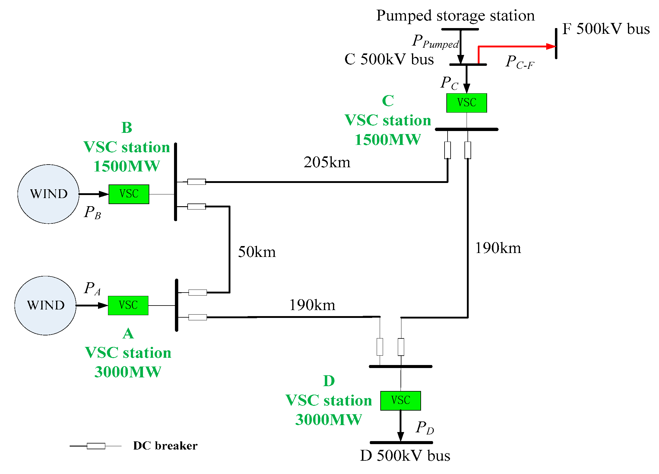
A MTDC grid project in a certain area, with three ±500 kV sending-end VSC stations, is discussed as the test benchmark. The installed capacity is 3000 MW for Station A and 1500 MW for Station B and C respectively. A ±500 kV receiving-end VSC Station D has a capacity of 3000 MW. Equipped with DC circuit breaker and DC line protection devices, this circular four-terminal network is designed and constructed for large-scale wind power and pumped storage hydropower transmission. The installed capacity of wind power pooling at the VSC station A and B is 150% of the installed capacity of the corresponding station. The VSC Station C is connected to an 1800 MW pumped storage hydropower station, as shown in Figure 1.

Figure 1.
The multi-terminal direct-current (MTDC) grid configuration.
The CVCF control of isolated converter is adopted for Station A and B, the constant DC voltage control is used in Station C to balance the active power of the MTDC grid, whereas the constant active power control is adopted for Station D. Ignoring the DC transmission consumption, the power balance relation of MTDC is shown as follows:
All the variables in Equation (1) consist of two parts:
represents the scheduled power of pumped storage station and Station D, the predicted wind power pooled in Station A and B, the calculated initial power of Station C based on the above mentioned power values, and is the deviation power between the actual power
and so called basic power
. It is known, as set out previously the control strategy of MTDC that, and
equal 0 and
and are the variation between the actual wind power and predicted wind power. As the actual power and basic power are balanced without considering the DC transmission consumption, the following equations can be obtained through Equations (1) and (2):
The MTDC has two links to the main grid, one is D 500 kV bus and the other is C−F AC 500 kV transmission line. As Pd can be a constant value, the key to transmit the wind power steadily through MTDC is to control PC−F. It can be seen from Equation (3) that can be controlled by properly arranging and in dispatch time interval according to the predicted wind power fluctuation [13]. However, significant can still exist as a result of unpredicted wind power fluctuation. Take several large wind farms with a total of 2150 MW (equal to the wind power installed capacity pooled in station B) installed capacity as an example. The maximum unpredicted wind power fluctuation could reach to 550 MW in one day. If the installed capacity of the main grid is relatively small, the unpredicted wind power fluctuation will cause severe frequency fluctuations in the main grid. As a result, it is necessary to alleviate the fluctuations that always occur over a shorter time interval.
2.2. The Fluctuation Characteristic of Large-Scale Wind Power Generation
Since the smooth delivery of large-scale wind power to the main grid is the main goal of the constructed MTDC network, the fluctuation characteristic of wind power pooling at station A and B is of great significance and needs to be thoroughly analyzed. More importantly, the short-time characteristic is closely related to the design of the fluctuation regulation scheme.
Normally the variability characteristics of wind power are investigated using a probability method [14,15]. The maximum fluctuation within a fixed time period was used to form a power fluctuation sequence. In particular, let us assume that the sampling interval of wind power is T0, then the maximum power fluctuation sequence within a time period of T = N*T0 can be expressed as:
where, is the current wind power pooling at a certain station in region B when t = i. Assume T0 to be 1 min and the total length of wind power sequence to be M. Thus, the maximum power fluctuation sequence with a length of M–N can be obtained.
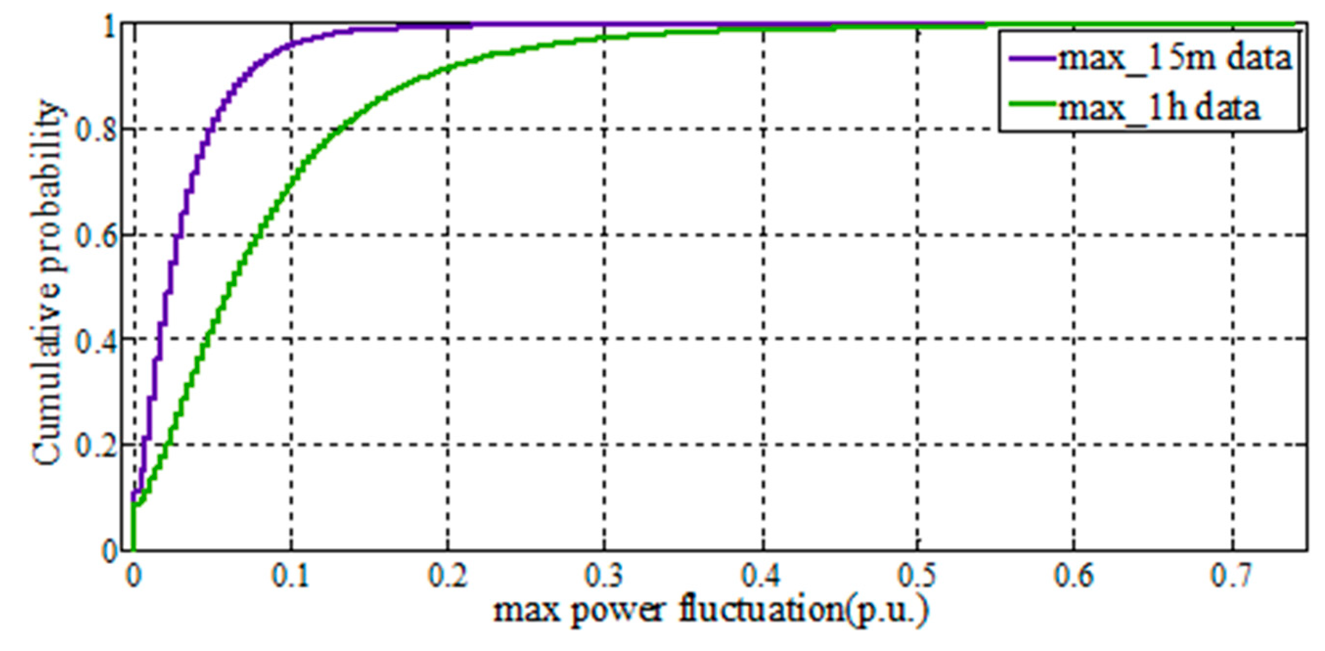
First of all, the characteristic of the maximum wind power fluctuation in region B was analyzed through the probability distribution of the corresponding maximum power fluctuation sequence within a time period T of 15 min and 60 min respectively. The obtained cumulative distribution is shown in Figure 2. It can be seen that, when T = 15 min, the probability of a maximum power fluctuation less than 0.094 (p.u.) is 95%, whereas the probability of the maximum fluctuation less than 0.161(p.u.) is 99%. Comparatively when T = 1 h, the probability of the maximum fluctuation less than 0.247 (p.u.) is 95% whereas the probability of the maximum fluctuation being less than 0.433 (p.u.) is 99%. However, the maximum power fluctuation for a single wind farm is much larger and could reach 1 (p.u.) compared to the aforementioned maximum fluctuation range. This means the geographical smoothing effect (or the cluster effect) could significantly reduce the variability of wind power output when transmitting integrated large-scale wind power. The aforementioned fluctuation characteristic in dispatch time interval will be key to designing the to alleviate the predicted wind fluctuation. This work is the foundation of this paper but will not be expressed in detail.
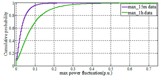
Figure 2.
The cumulative probability of maximum wind power fluctuation within a different time period.
The short-time power fluctuation rate was obtained by taking N = 1 in the power fluctuation sequence equation, that is a power fluctuation within 1 min. The cumulative probability distribution analysis of the instantaneous power variation between the actual power and predicted wind power can then somewhat represent which is just a smaller part of .A similar procedure was conducted using the same data when analyzing the short-time power fluctuation characteristic. As shown in Figure 3, although the largest instantaneous fluctuation rate is 0.318 (p.u./min), 95% of the instantaneous fluctuation rate is less than 0.014 (p.u./min) and 99% of the instantaneous fluctuation rate is less than 0.021 (p.u./min). So the instantaneous fluctuation rate is relatively small most of the time.
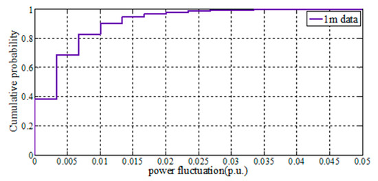
Figure 3.
The cumulative probability of wind power fluctuation within 1 min.
3. Virtual Frequency Control Strategy of Islanded VSC Station
3.1. CVCF Control of VSC Station in Islanded Mode
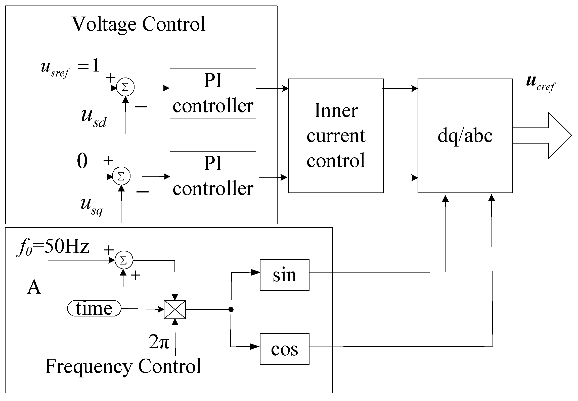
Frequency and voltage are the most important features of the AC power system. When connecting an islanded system to the MTDC grid, the VSC station will normally provide the AC voltage us with a constant frequency (f0 = 50 Hz) and constant amplitude for the islanded system. Such a control strategy is regarded as CVCF control and its logic diagram is shown in Figure 4. In the AC voltage control unit, the reference value of d-axis voltage usd was set as the constant amplitude usref (usually set to 1) to calculate the reference value of d-axis current, whereas the reference value of q-axis voltage usq was set to 0 to calculate the reference value of q-axis current. Then the dq-axis reference value of the voltage at the AC-side of the converter is obtained by the inner current control unit. In the frequency control unit, the sine and cosine waves with constant frequency 50 Hz (f0) were used for conducting the inverse PARK transformation to calculate the three-phase reference value ucref of the voltage at the AC-side of the converter.

Figure 4.
The constant voltage constant frequency (CVCF) control diagram of islanded voltage source converter (VSC) station.
3.2. VF Control of the Islanded VSC Station
Under the CVCF control strategy, the power output from the VSC station in islanded mode is not regulated so the total active power delivered by the VSC station is the sum of wind power generated in real time. However, a constancy of frequency at 50 Hz is maintained for the connected islanded system regardless of the variation of wind power (taking no account of the occurrence of oscillation). Therefore, the most state-of-the-art PFR technique [16,17,18] developed for a wind power station in a synchronous AC system cannot be used in an islanded system. It is readily for us to make some effort to simulate the PFR which can decrease the active power deviation between generation and load in a synchronous AC system. In the islanded system, the actual wind power output can serve as the generation, and the scheduled (e.g., predicted) wind power out can serve as the load.
For this purpose, a supplementary VF control strategy is designed on top of the conventional CVCF control to produce a virtual frequency, which serves as the new benchmark frequency for the AC voltage at the VSC station. This allows the frequency of the islanded system to vary with the deviation of the actual power output from the scheduled power output, allowing the PFR technique adopted for wind power in synchronous AC grid to be applied to the islanded system to realize the self-regulation of active power at the VSC station.
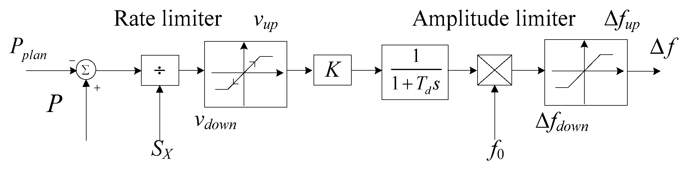
The VF control diagram is shown in Figure 5 where the power difference between the real-time power P of the VSC station and the scheduled power Pplan at any given time is calculated and normalized per unit as the input for the rate limiter module. Sx represents the nominal capacity of VSC station X. As previously mentioned in Section 2, due to the cluster effect of large-scale wind power integration, that the maximum power fluctuation rate of wind power at the VSC station is approximately 30% of its installed capacity per minute, any fluctuation rate higher could be a result of failure of either the VSC station or the power transducer. In short, the normal power fluctuation rate should be less than 0.005 (p.u./s). Here the rate limit is set to 0.0075 (p.u./s) since the total installed capacity of wind farms is 1.5 times that of the VSC station itself. Hence, vup and vdown respresent the increasing rate limit and decreasing rate limit respectively. This limit is multiplied by the frequency-power factor K and enters a one-order filter with the time constant Td. Finally, it is multiplied by f0 to obtain the nominal frequency and further processed in the amplitude limiter module with upper limit and lower limit to get the frequency difference . The virtual frequency will be obtained by adding to f0 at point A in Figure 4.
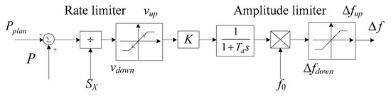
Figure 5.
Virtual frequency (VF) control diagram.
3.3. PFR Control of the Wind Farms and Self-Regulation Scheme of Power Fluctuations
The PFR control is a key part of the self-regulation scheme. Although its full realization of a wind farm will not be discussed here in detail, the basic control diagram is also given to introduce some key parameters, which is closely related to the following analysis. It is shown in Figure 6 that the PFR control is similar to the VF control and also realized in per unit system. The only different module is to substitute the rate limiter in VF control to dead zone in PFR control.
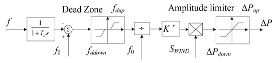
Figure 6.
Primary frequency regulation (PFR) control diagram.
By combining the VF and PFR control, the self-regulation of the active power fluctuation at the islanded VSC station can be realized as follows: once the total active power P of wind power pooling at the VSC station falls short of the scheduled total active power Pplan, a negative is produced with VF control and the frequency of isolated power system decreases along with the virtual frequency, then PFR control at the wind farms (if not in the maximum power generation mode) reacts to generate more power to compensate the power shortage to further restore the frequency close to f0. On the other hand, when P is greater than Pplan, with VF control the frequency of the isolated power system increases by a positive and PFR reacts to reduce the power generation at the wind farms thus the frequency could also decline to some extent. With such a self-regulation scheme, the sending-end VSC station A and B of a MTDC network could regulate the power fluctuation of the connected islanded system and deliver the power scheduled by the day-ahead generation plan.
4. The Steady-State Analysis of the MTDC Grid with VF + PFR Control
In order to observe the self-regulation effect on power fluctuation by the proposed scheme, one of the two islanded VSC stations and its connecting islanded system has been selected for further analysis, given they are very similar. Thus, these assumptions are given in the following analysis on the basic of the test benchmark introduced in Figure 1:
- VSC Station B was selected and five wind farms connected to this VSC station. The capacities of these wind farms are 300, 450, 250, 500, and 750 MW respectively.
- In order to evaluate the self-regulation effect of the power fluctuation in VSC Station B independently, the actual power of the wind farms connected to VSC Station A will conform with their day-ahead predicted power.
- the power consumption of the MTDC is neglected.
4.1. Self-Regulation Effect of the Power Fluctuation with Different Control Parameters
Although some parameters have already been discussed and settled in Section 3, the others are still adjustable and play important roles in the self-regulation effect of the power fluctuation.
Firstly, to avoid the off-grid accident under VF control, the values of the amplitude limiter in VF control should be set according to the frequency continuous operating range of the wind farms. It is restricted to 49.5~50.2 Hz in the current criterion in China, and is about to expand in the near future. Secondly, the vital parameters K and K’ in VF + PFR control are set with reference to the speed governing droop coefficient which is about 3%~6% in the PFR control of the conventional synchronous power station at first, and then adjusted according to the electromagnetic transient simulation to avoid some unstable oscillation. Thirdly, the amplitude limiter in the PFR control is discussed with the assumption that the wind farms are in or not in maximum power generation mode. Finally, the impact of different values set in the dead zone of the PFR control is also discussed.
To achieve a simpler and clearer analysis, the parameters in the PFR control of different wind farms are the same and hence the PFR control in Figure 6 is treated as one equivalent PFR controller of all the wind farms. The proportion of the total capacity of the wind farms that are equipped with PFR to the capacity of VSC Station B is marked as m%. The SWIND can then be regarded as the total capacity of wind farms with PFR, and the following relation can be readily obtained:
Consequently, and are the total increase and decrease in capacity respectively. With another assumption that the per unit active powers of the five wind farms are the same, and can be expressed as:
where Pup% represents the active power increasing ability of the wind farms with PFR.
4.1.1. Different Values of the Amplitude Limiter in VF Control
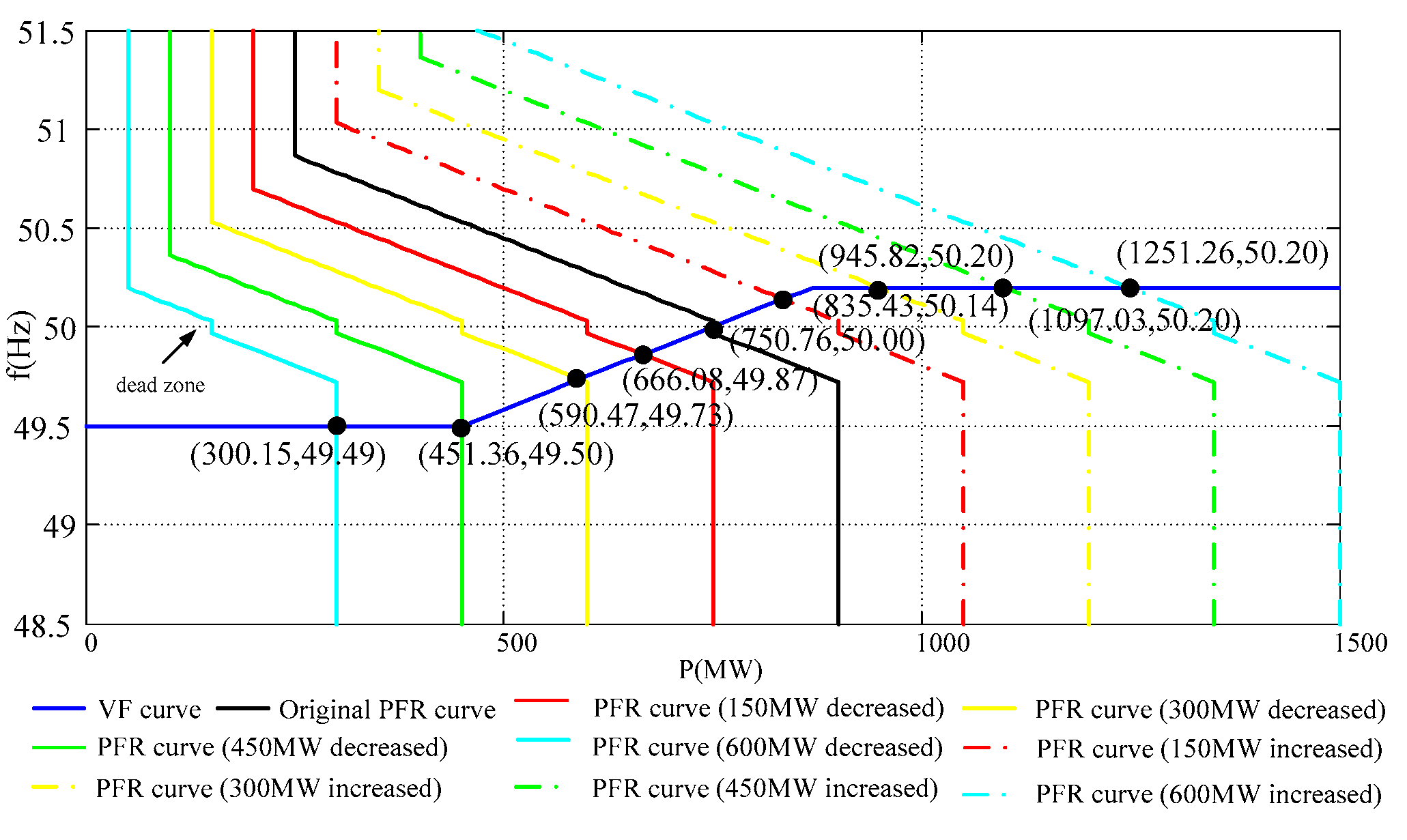
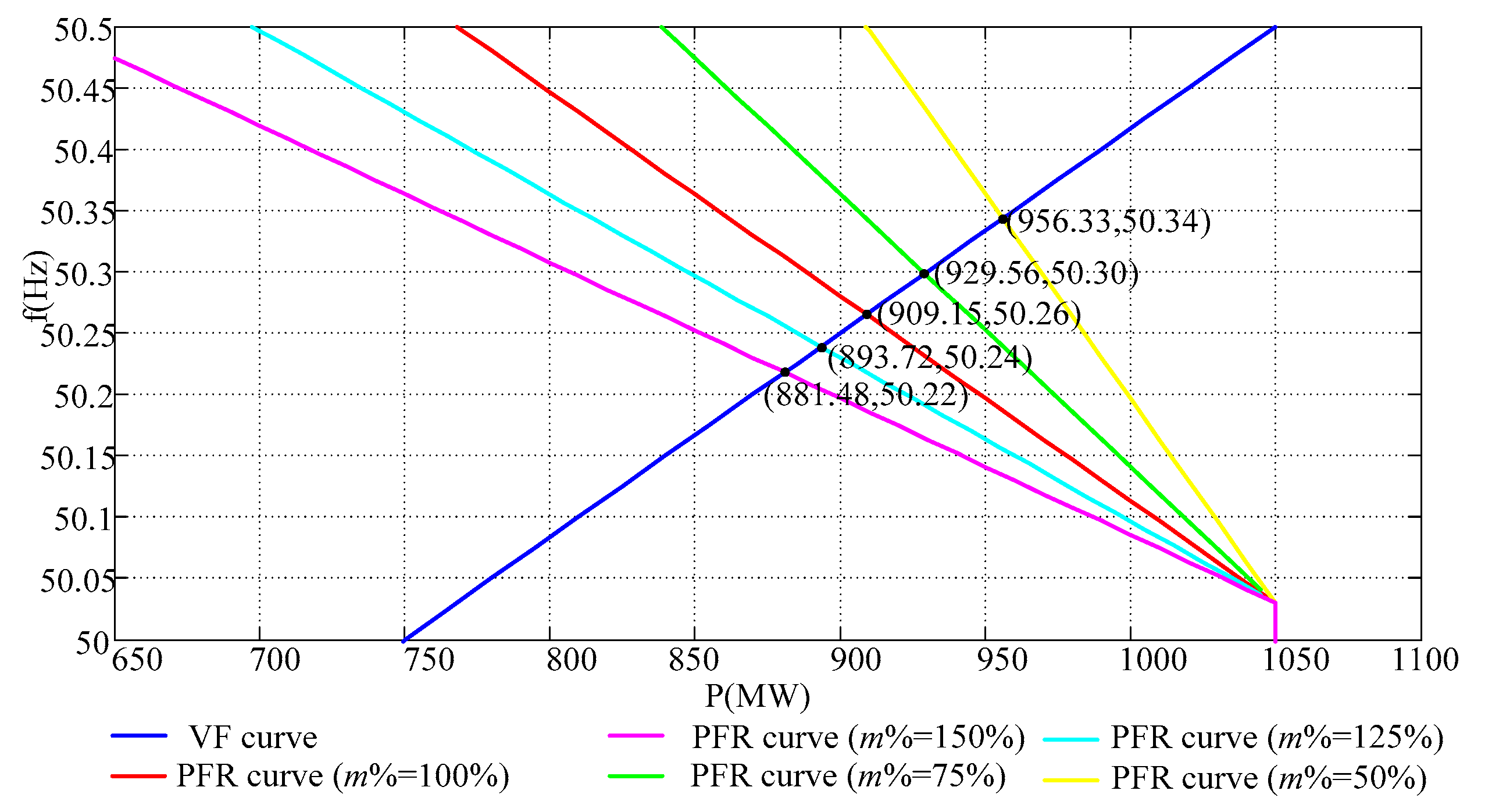
The tentative control parameters of Group 1 are shown in Table 1 when some initial conditions are listed in Table 2. The is set as 0.2 Hz and is −0.5 Hz initially. According to these parameters, the frequency-power anti-droop characteristic curve of VSC station B is shown in Figure 7. Several PFR characteristic curves of the wind farms are also shown in Figure 7 under the conditions that are ±150, ±300, ±450, and ±600 MW. The new frequency-power operation points of the islanded system can be then obtained from the intersections of these curves.

Table 1.
The parameters in VF + PFR control (Group 1).
Table 2.
The initial conditions.
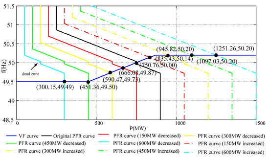
Figure 7.
VF curve and PFR curves (control parameters Group 1).
It can be readily identified that the self-regulation proportion of power fluctuation is about 44% when the intersections are neither in the limitation area of the VF curve nor in the limitation areas of the PFR curves. When is more than +300 MW, the self-regulation proportions reduce to different degrees caused by the amplitude limiter either in VF control or in PFR control. Detailed information is shown in Table 3.
Table 3.
The self-regulation proportions of power fluctuations (different VF amplitude limiter).
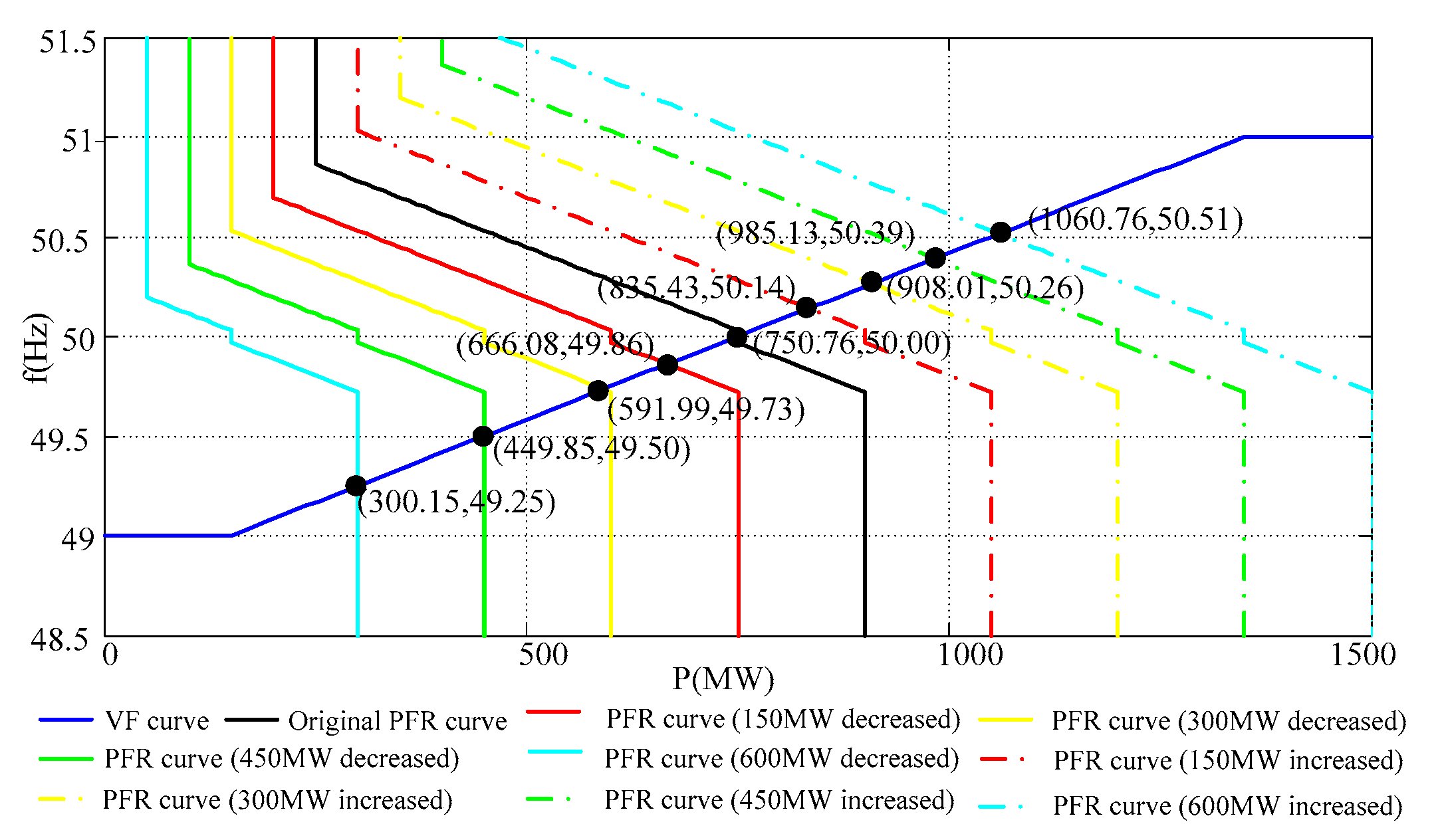
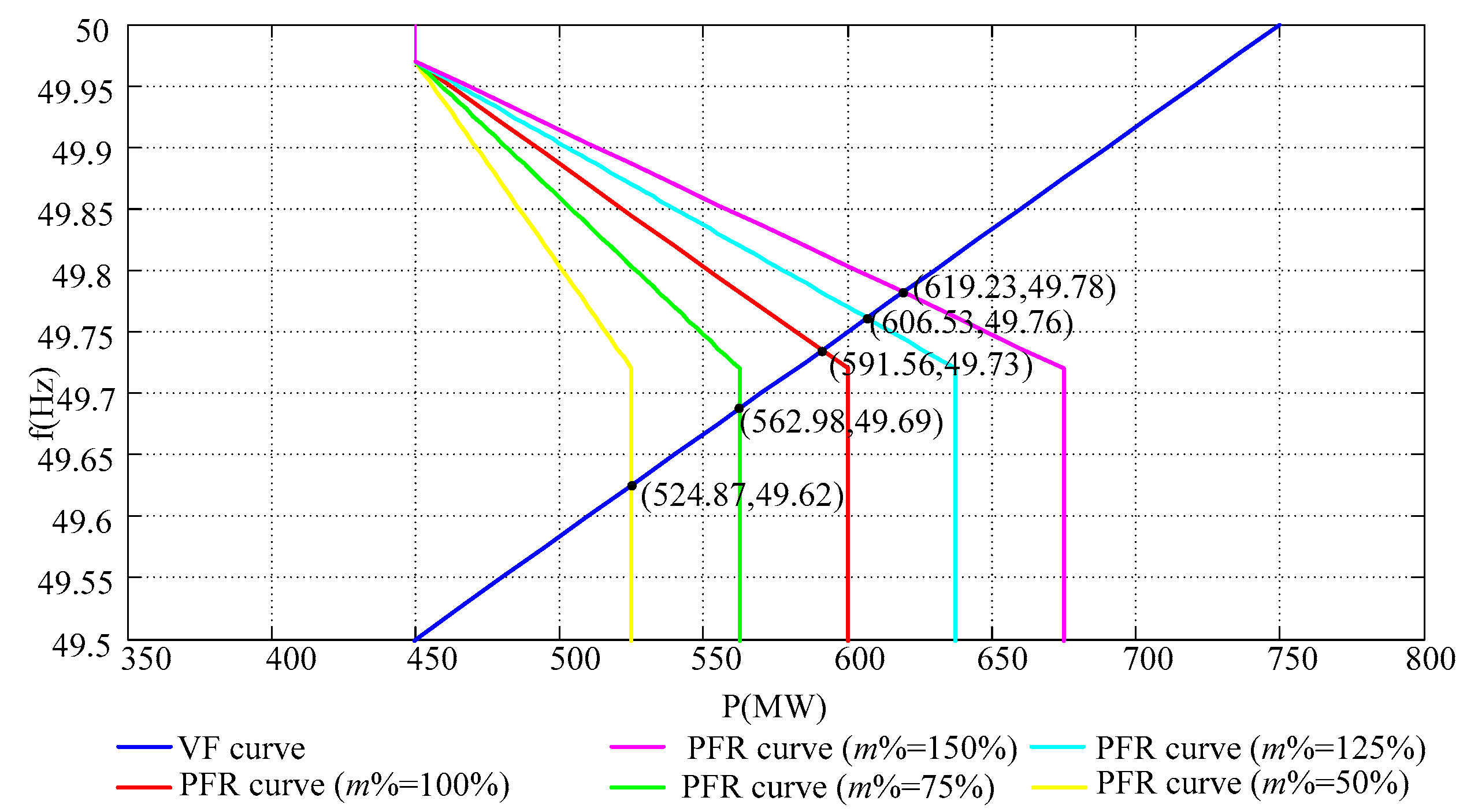
If the frequency continuous operating range of the wind farms expand to 49~51 Hz, the corresponding VF curve and PFR curves are shown in Figure 8. In order to compare the impacts of the different amplitude limiters in VF control, the self-regulation proportions are also listed in Table 3. It can be concluded from the comparison that the increased power fluctuation can be better regulated if the frequency continuous operating range of the wind farms expand.
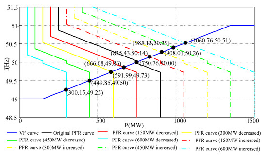
Figure 8.
VF curve and PFR curves (control parameters Group 1 and VF amplitude limiter expands to 49~51 Hz).
4.1.2. Different Values of K and K’ in VF + PFR Control
The tentative principle of setting K and K’ is that their product is 1. The electromagnetic transient simulation result indicates that K can’t be set larger than 0.05. The self-regulation proportion when the control pair K and K’ being set as 0.025 and 40 is compared to that being set as 0.05 and 20 in the former analysis as is shown in Figure 9. Take one condition, that unpredicted power fluctuation is +150 MW for instance, and the self-regulation effect with the initial control parameters is better than that with the newly proposed parameters which can be concluded from Table 4.
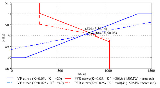
Figure 9.
VF curves and PFR curves (K = 0.05, K’ = 20 and K = 0.025, K’ = 40).
Table 4.
The self-regulation proportions of power fluctuations (different K and K’).
4.1.3. Different Values of Dead Zone in PFR Control
The value of the dead zone in the PFR control also affects the self-regulation effect. Similarly, the setting of its value is restricted by the electromagnetic transient simulation result that fdead cannot be set smaller than 0.03. The self-regulation proportion when fdead is set as 0.06 is compared to that being set as 0.03 in the former analysis. Take the same condition as in the last comparison for instance, the self-regulation effect with the initial control parameters is still better than that with the newly proposed parameters which can be concluded from Table 5.
Table 5.
The self-regulation proportions of power fluctuations (different fdead).
4.1.4. Different Values of the Amplitude Limiter in PFR Control
The amplitude limiter in PFR control has the most significant influence on the self-regulation effect practically, since the self-regulation is finally realized by the PFR control in wind farms. If the wind farms are already operating in the maximum power generation mode, they cannot increase their active power in the long term. This means in Table 1 is adjusted to 0 MW and all the PFR curves in Figure 7 to Figure 10 only retain their left part taking the dead zone as the boundary. As a result, only the positive unpredicted wind power fluctuation can be regulated.
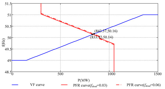
Figure 10.
VF curve and PFR curves (fdead = 0.03 and fdead = 0.06).
4.2. Self-Regulation Effect of Power Fluctuations with Different m%
Some of the wind farms in islanded systems have been operated for a long time, so it is uncertain whether the PFR control can be added to these wind farms. Planned wind farms should be forced to add PFR control. As a result, the proportions of the wind farms that are equipped with PFR is hard to determine which means m% is a variable.
Some of the rudimentary VF and PFR control parameters have been established through the discussion in the previous analysis. Nevertheless, the variable m% would not only have significant influence on the self-regulation effect by itself, but also would affect some PFR control parameters according to Equation (7). Take one condition that unpredicted power fluctuation is ±300 MW for instance, the self-regulation effect becomes better as the m% increases. It also can be seen from Figure 11, Figure 12 and Table 6 that the self-regulation proportion changes more markedly when m% is relatively small and increases slowly when m% is over 100%.
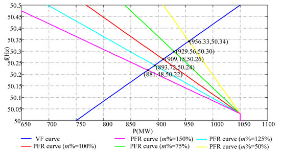
Figure 11.
VF curve and PFR curves (ΔPB = +300 MW).
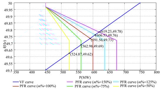
Figure 12.
VF curve and PFR curves (ΔPB = −300 MW).
Table 6.
The self-regulation proportions of power fluctuations (different m%).
4.3. Twenty-Four-Hour Simulation of the MTDC Grid with Self-Regulation Scheme
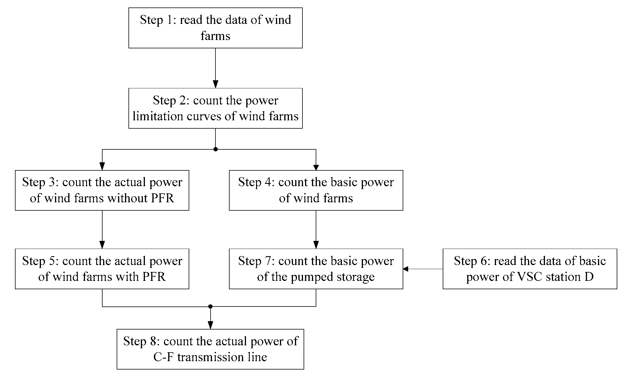
With the conclusion drawn from the previous discussion, a twenty-four-hour simulation of the possible operating state of the MTDC grid is obtained by a specific program. The steps of this program are shown in Figure 13. In Step 1, the predicted power and the initial actual power of five wind farms are acquired according to the actual operating data of a large wind farm in five days respectively. In Step 2, the power limitation curve represents the active power limitation of a wind farm and it is obtained by the security constrains () according to the reference [19]. In Step 3, the actual power without PFR of a wind farm is counted by the initial actual power data and its power limitation curve. Similarly, the basic power of a wind farm is then counted by the initial predicted power data and its power limitation curve in Step 4. In Step 5, the actual power with PFR of a wind farm is counted by the method used in the previous analysis. After reading the data of the basic power of the VSC Station D in Step 6, the basic power of the pumped storage station can be counted in Step 7 according to Equation (3) with the ideal target that the power of the C−F transmission line is zero. At last, the actual power of the C−F transmission line is obtained by Equation (4) in step 8.
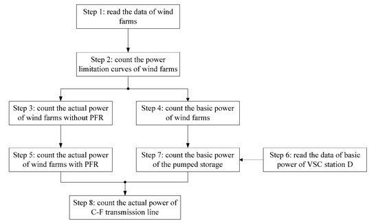
Figure 13.
The Steps of the MTDC twenty-four-hour simulation program.
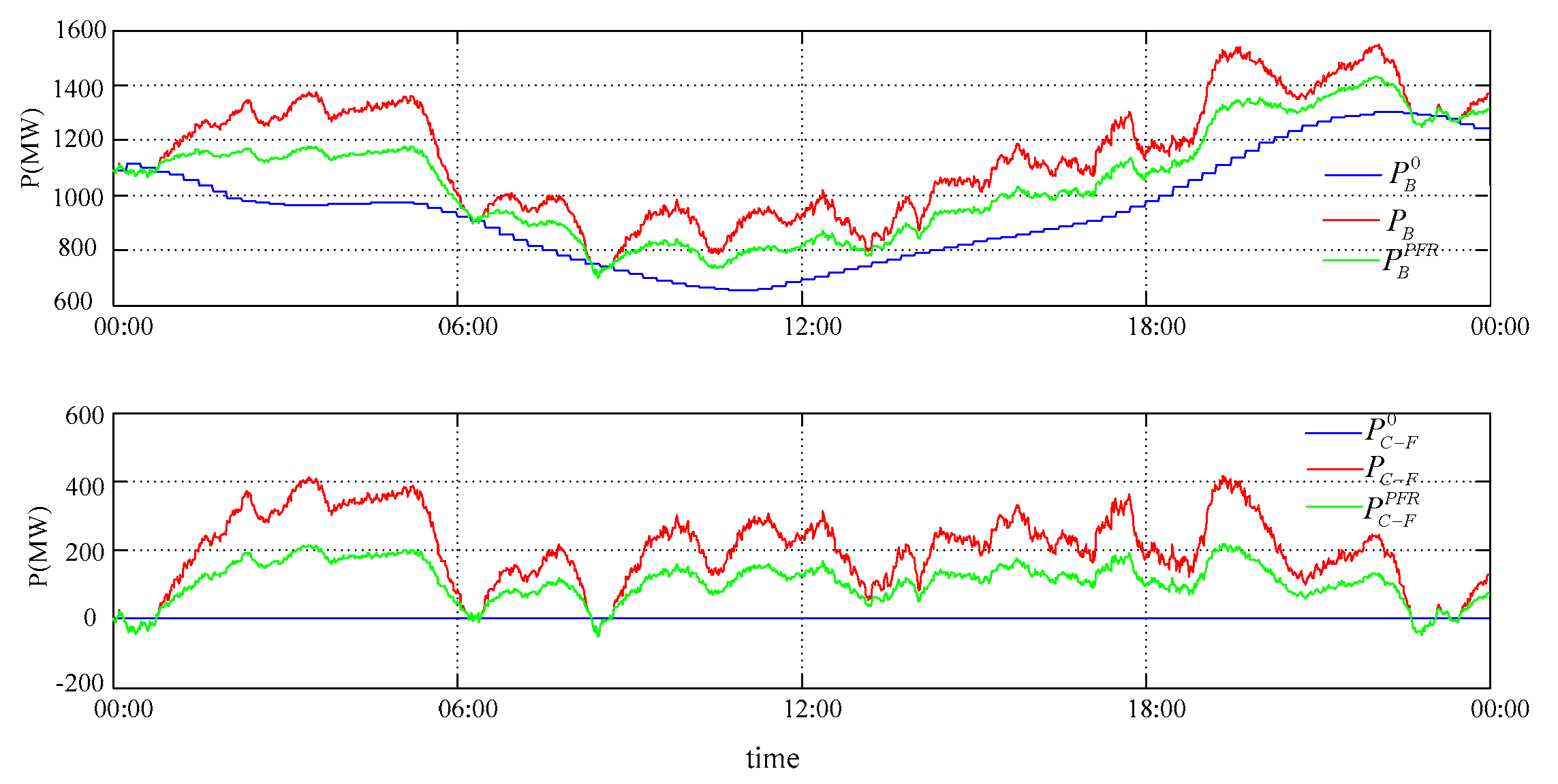
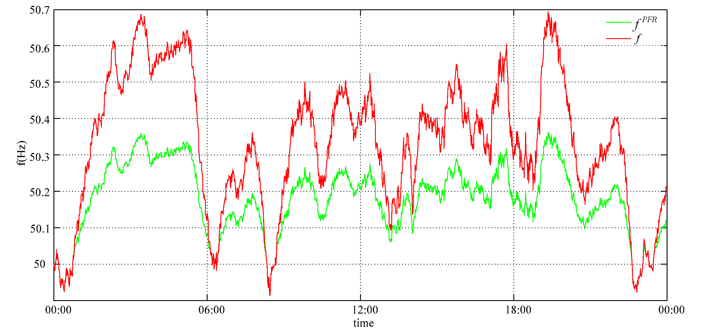
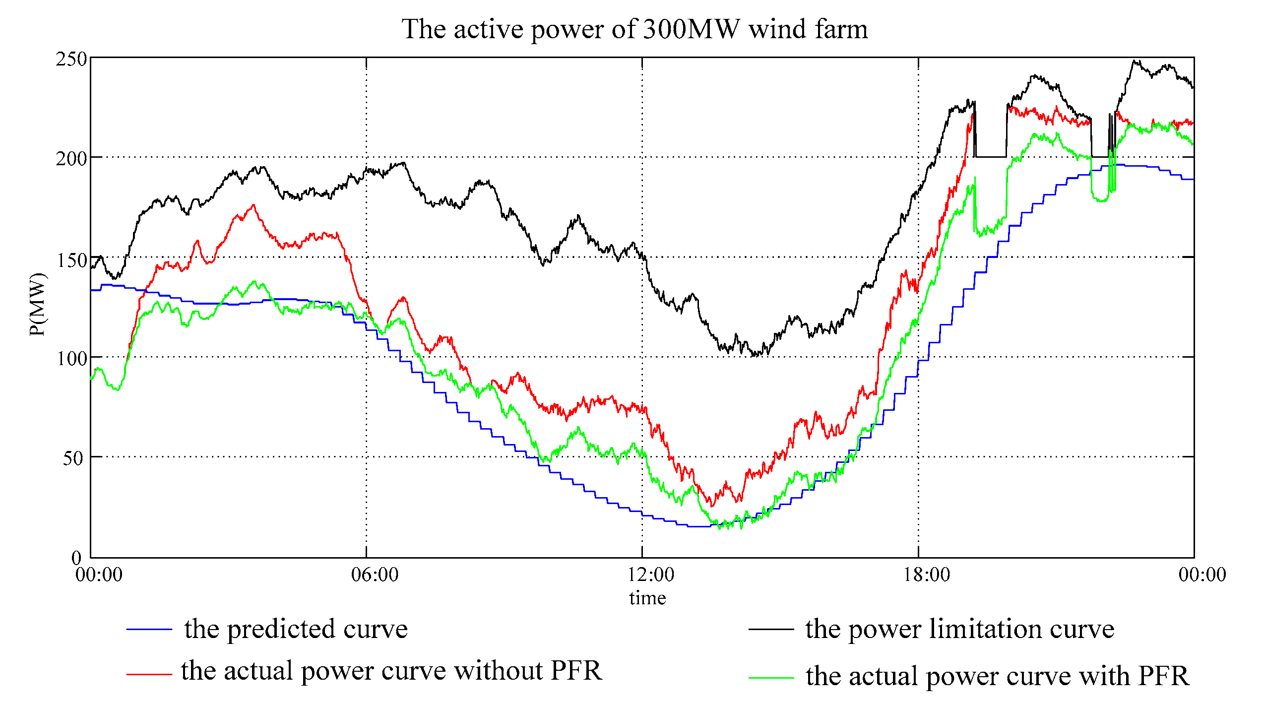
In the twenty-four-hour simulation, four wind farms are equipped with PFR but not the largest wind farm of 750 MW capacity which makes m% 100%. The VF and PFR control parameters are selected as in Table 1 except that and are set as . As can be seen in Figure 14, the variation between the basic power and the actual power of the VSC station B can be reduced by approximately half. Consequently, the power variation of the C−F transmission line can be reduced by half according to Equation (4). As a result of the VF + PFR control, the curve of the frequency of the islanded system is smoother compared to that without PFR control which is shown in Figure 15. Take the wind farm with 300 MW capacity, for instance; the predicted power, the power limitation, the actual power without PFR, and the actual power with PFR which are obtained in the supposed program are shown in Figure 16. It is worth noting that two notches in the power limitation curve are caused by the security constrains () and also influence the actual power curves with and without PFR.
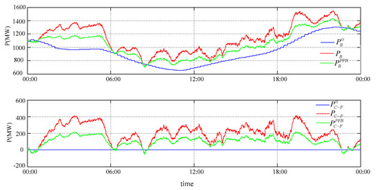
Figure 14.
The basic power, and actual power with and without PFR of VSC station B and the C−F transmission line.
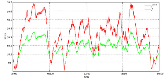
Figure 15.
The frequency of the islanded system with and without PFR control.
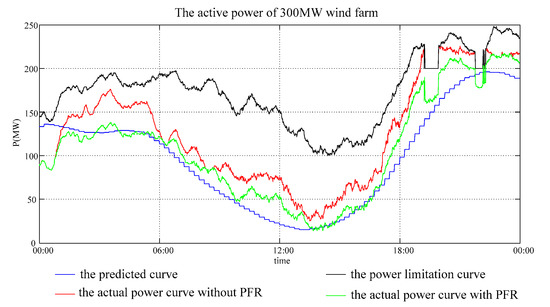
Figure 16.
The predicted power, the power limitation, the actual power without PFR and the actual power with PFR of the 300 MW wind farm.
5. Conclusions
In this paper, a self-regulation scheme of the wind power fluctuation was proposed towards the islanded system of a MTDC project in the certain area, and the following conclusions are drawn:
- Although the short-time power fluctuation of a single wind farm or PV station could reach 100%, the power fluctuation of the large-scale wind power stations will be much smoother due to the cluster effect. In our project, it is found that the maximum fluctuation rate reaches to 0.318 (p.u./min) which serves at the rate limit value for VF control, and 99% of instantaneous fluctuations rate falls within 0–0.021 (p.u./min). The unpredicted wind power fluctuation reaches 550 MW at most.
- The islanded VSC stations are mostly used in delivering offshore wind power. Traditionally the islanded VSC station adopts the CVCF control strategy. In this case, the active power fluctuation resulting from the wind power variability will be transmitted to the receiving-end grid. To mitigate such power fluctuation, a self-regulation scheme is developed in this paper combining VF control at the VSC station and PFR control at the wind farms.
- The control parameters of VF control and PFR control have a significant influence on the self-regulation effect. These parameters are carefully set based on a steady-state analysis as well as the electromagnetic transient analysis which may be introduced in the future. As a result, the self-regulation proportion can reach 56% in the best conditions. The analysis of the system variable m% indicates that the self-regulation effect could be accepted when about two thirds of the wind farms are equipped with PFR instead of all the wind farms.
In all, this paper has proposed a self-regulation scheme and analyzed and demonstrated its performance in mitigating the power fluctuation. With the renewable power penetration level growing higher in the grid and the more extensive use of HVDC transmission, the proposed scheme could be extensively applied serving as a supplementary control for the system stability.
Author Contributions
Conceptualization, H.W.; formal analysis, J.S.; data curation, Q.P.; writing—original draft preparation, J.S.; writing—review and editing, H.W.; supervision, X.Z. All authors have read and agreed to the published version of the manuscript.
Funding
This research received no external funding.
Conflicts of Interest
The authors declare no conflict of interest.
Abbreviations
| VSC | The Voltage Source Converter |
| HVDC | High Voltage Direct Current |
| AC | Alternative Current |
| DC | Direct Current |
| MTDC | Multi-Terminal Direct-Current |
| CVCF | Constant Voltage Constant Frequency |
| VF | Virtual Frequency |
| PFR | Primary Frequency Regulation |
References
- Renedo, J.; Garcia-Cerrada, A.; Rouco, L. Active Power Control Strategies for Transient Stability Enhancement of AC/DC Grids with VSC-HVDC Multi-Terminal Systems. IEEE Trans. Power Syst. 2016, 31, 4595–4604. [Google Scholar] [CrossRef]
- Arani, M.F.M.; Mohamed, Y.A.R.I. Analysis and Performance Enhancement of Vector-Controlled VSC in HVDC Links Connected to Very Weak Grids. IEEE Trans. Power Syst. 2017, 32, 684–693. [Google Scholar] [CrossRef]
- Pan, Y.; Yin, X.; Hu, J.; He, J. Centralized Exploitation and Large-Scale Delivery of Wind and Solar Energies in West China Based on Flexible DC Grid. Power Syst. Technol. 2016, 40, 3621–3629. [Google Scholar]
- Tang, G. HVDC Power Transmission System Based on Voltage Source Converters; Electric Power Press: Beijing, China, 2010; pp. 89–91. [Google Scholar]
- Shi, G.; Wu, G.; Cai, X.; Chen, Z. Coordinated control of multi-terminal VSC-HVDC transmission for large offshore wind farms. In Proceedings of the 7th International Power Electronics and Motion Control Conference, Harbin, China, 2–5 June 2012; pp. 1278–1282. [Google Scholar]
- Zhang, Z.; Li, X.; Chen, M.; Huang, Y.; Xu, S.; Zhao, X. Research on Critical Technical Parameters of HVDC Circuit Breakers Applied in Nan’ao Multi-Terminal VSC-HVDC Project. Power Syst. Technol. 2017, 41, 2417–2422. [Google Scholar]
- Rao, H.; Li, L.; Guo, J.; Li, X.; Chen, M.; Xu, S. Analysis on the Main Wiring of Nan’ao VSC-HVDC Transmission System. South. Power Syst. Technol. 2012, 6, 1–5. [Google Scholar]
- Hu, X.; Liang, J.; Rogers, D.J.; Li, Y. Power Flow and Power Reduction Control Using Variable Frequency of Offshore AC Grids. IEEE Trans. Power Syst. 2013, 28, 3897–3905. [Google Scholar] [CrossRef]
- Nanou, S.I.; Papathanassiou, S.A. Grid Code Compatibility of VSC-HVDC Connected Offshore Wind Turbines Employing Power Synchronization Control. IEEE Trans. Power Syst. 2016, 31, 5042–5050. [Google Scholar] [CrossRef]
- Sakamuri, J.N.; Hansen, A.D.; Cutululis, N.A.; Altin, M.; Sorensen, P.E. Coordinated fast primary frequency control from offshore wind power plants in MTDC system. In Proceedings of the IEEE International Energy Conference (ENERGYCON), Leuven, Belgium, 4–8 April 2016; pp. 1–6. [Google Scholar]
- Guan, M.; Zhang, J.; Liu, Q.; Yang, L.; Zheng, X.; Wu, G. Generalized Control Strategy for Grid-connected and Island Operation of VSC-HVDC System. Autom. Electr. Power Syst. 2015, 39, 103–109. [Google Scholar]
- Shah, R.; Barnes, M.; Preece, R. Offshore AC grid management for an AC integrated VSC-HVDC scheme with large WPPs. In Proceedings of the IEEE Power and Energy Society General Meeting (PESGM), Boston, MA, USA, 17–21 July 2016; pp. 1–5. [Google Scholar]
- Li, W.; Zhang, J.; Bu, G.; Wang, H.; Zhao, B. A coordinate complementary optimization control scheme between pumped storage station and large-scale new renewable integrated through VSC-MTDC. Power Syst. Prot. Control 2017, 45, 130–135. [Google Scholar]
- Hou, Y.H.; Fang, D.Z.; Qi, J.; Li, H.B.; Niu, W.; Yang, T. Analysis on Active Power Fluctuation Characteristics of Large-Scale Grid-Connected Wind Farm and Generation Scheduling Simulation Under Different Capacity Power Injected From Wind Farms Into Power Grid. Power Syst. Technol. 2010, 34, 60–66. [Google Scholar]
- Yü, Y.; Lu, G.; Xie, C.; Dai, H.; Yu, Z.; Yan, J. Online Probabilistic Security Assessment Considering Centralized Integration of Large Scale Wind Power. Power Syst. Technol. 2018, 42, 1140–1148. [Google Scholar]
- Liu, J.; Yao, W.; Wen, J.; Huang, Y.; Liu, Y.; Ma, R. Prospect of Technology for Large-Scale Wind Farm Participating Into Power Grid Frequency Regulation. Power Syst. Technol. 2014, 38, 638–646. [Google Scholar]
- Wang, Z.; Wu, W. Coordinated Control Method for DFIG-Based Wind Farm to Provide Primary Frequency Regulation Service. IEEE Trans. Power Syst. 2018, 33, 2644–2659. [Google Scholar] [CrossRef]
- Zhaozhi, Z. Control Strategy of Wind Farm for Power System Auxiliary Frequency Regulation. Ph.D. Thesis, Lanzhou University of Technology, Lanzhou, China, 2016. [Google Scholar]
- Zhuo, J.; Jin, X.; Deng, B.; Shang, X.; Zhao, L.; Tang, W.; Liu, C. An Active Power Control Method of Large-Scale Wind Farm Considering Security Constraints of Tie Lines. Power Syst. Technol. 2015, 39, 1014–1018. [Google Scholar]


© 2020 by the authors. Licensee MDPI, Basel, Switzerland. This article is an open access article distributed under the terms and conditions of the Creative Commons Attribution (CC BY) license (http://creativecommons.org/licenses/by/4.0/).