Abstract
Throughout the developing world, most remote and isolated communities are still without reliable electricity in the twenty-first century, and this is primarily due to the high cost of grid extensions. In communities that do have electricity, they usually rely on diesel generators, though these have high operating and maintenance costs, while also polluting the environment. A more sustainable approach is to deploy microgrids, however, microgrids have a high upfront cost, which is a major obstacle, especially in rural areas of developing countries. This study aims to investigate the parameters that can be influenced to make microgrids more economical for rural electrification. Through sensitivity analyses, five key policy and technology parameters were identified. They include real discount rates, diesel prices, grants, battery chemistry, and operating strategies. The system was then redesigned using scenarios formulated by varying these parameters. Results show that the parameters affect the configuration, levelized cost of energy (LCOE), renewable energy penetration (REP), and pollutant emissions. The study uses three remote communities in the Beni Department of Bolivia as case studies. MDSTool was used as a modeling framework to design the microgrids. The unique insights and lessons learned during the design process are discussed at length because these may be valuable for future microgrid designs for remote communities.
1. Introduction
The benefits of rural electrification are well-documented in the literature [1] and include economic, health, educational, social life, and environmental benefits. The economic benefits include an increase in the number of enterprises in the newly-electrified communities, as reported in Bolivia [2]. In a similar study in [3], the enterprises operated by rural households in Indonesia increased by 43% after gaining access to electricity. The health benefits of having reliable electricity were reported in [4], where 35% of newly solar-electrified households in rural Namibia reported an improvement in health [4]. Electrified communities will use less kerosene for lighting and cooking, which, in turn, was noted to reduce fire accidents [5] and prevent health conditions such as lung disease and poisoning [6]. Access to electricity has also been widely reported to immensely benefit education. For example, the primary school completion rate more than doubled for households with access to electricity in rural Nicaragua [7], and similar findings were reported in Vietnam [8] and South Africa [9]. Access to electricity may improve social interactions. Villagers in rural Zambia have greater access to news outside of their community through TV and radio as a result of having reliable access to electricity [10], and another study in Kenya had similar conclusions [11].
Despite these benefits, however, more than one billion people, or about 13% of the world’s population, do not have electricity in the 21st century [12]. The United Nations SDG7 calls for universal access to electricity by 2030 [13]. If the current population trends and policies continue, this target will not be achieved; it is currently estimated that up to 674 million people will still be without electricity by 2030 [14]. The majority of these populations live in Sub-Saharan Africa, Latin America, and South Asia. They are mostly living in remote areas far away from the central grid, thereby making grid extensions economically infeasible. The installation of diesel generators can be a quick way to provide electricity to these communities. However, the high fuel price, significant operation and maintenance cost, and the rising concern regarding pollutant emissions are some of the factors making this approach unpopular.
A more sustainable approach is to deploy microgrids that use renewable energy sources (RES), such as solar photovoltaic (PV) and wind turbines (WT) [15]. Microgrids can significantly reduce operation and maintenance costs, are more sustainable, and produce less harmful emissions, among other benefits [16]. However, the considerable upfront cost and risks associated with renewable energy investments are the main obstacles to their widespread adoption in these communities [17]. To overcome these obstacles, various rural electrification initiatives were undertaken in developing countries, with mixed results. Some of these initiatives include Lighting Africa [18] in Sub-Saharan Africa, Luz para todos (“Light for all”) in Brazil [19], and the IDCOL program in Bangladesh [20,21], among many others [22].
This study aims to find the parameters that most affect the microgrid investment for rural electrification. Through sensitivity analyses, five key policy and technology parameters were identified that most affect the optimal design of remote microgrids. Scenario analyses were used to find the impacts of these five parameters on the configuration, levelized cost of energy (LCOE), renewable energy penetration (REP), and pollutant emissions.
The study was conducted by designing microgrids in three rural communities located near the Bolivia-Brazil border in the Amazon, all located in the Beni Department of Bolivia. The three communities were visited by the authors of this study for data collection and site assessment. This visit was one of the crucial elements of this research, as most studies about remote microgrids (reviewed in the next section) rely solely on estimated data, which may not accurately reflect the real situations faced by communities. MDSTool was used as a modeling framework for the design [23].
In summary, this study has the following main contributions:
- We offer a model that uses various operating strategies to simulate the annual operation of remote microgrids, enabling the study of the impacts that different parameters have on the optimal design of remote microgrids.
- We analyzed case studies of three remote communities in Bolivia, making our findings more rigorous. Unlike grid-connected microgrids, where the site characteristics can differ significantly due to different utility tariffs, local ancillary services, and various regulatory and policy differences (i.e., net metering and demand response), remote microgrids have fewer site differences. Therefore, the conclusions in this study can be easily extended to other remote microgrids in different locations.
- Through sensitivity analyses, we identified five key policies and technological parameters that had the most impact on the design of remote microgrids. Detailed scenario analyses were used to find the effects of these parameters on the configuration, LCOE, REP, and pollutant emissions.
The rest of the paper is structured as follows: Section 2 presents a literature review on the feasibility analysis of microgrid in remote communities. In Section 3, we introduce the design methodology and introduce the modeling tool. The case studies are introduced in Section 4. Results and discussion are presented in Section 5. The paper concludes in Section 6.
2. Related Work
A thorough review of the available literature on the feasibility of microgrids in remote communities was presented in this section. The review was completed to identify the knowledge gap and develop supporting arguments. The reviewed studies are from various developing countries from all regions of the world, conducted in the last two decades. All the reviewed studies follow either optimization-based approach or simulation-based approach to microgrid design. The optimization-based approach uses an optimization model to find the optimal sizes of DERs in the microgrid. On the other hand, a simulation-based approach finds the optimal DERs sizes by using performance and economic model to simulate the operation and economics of the system, respectively.
The studies that follow the optimization-based approach can be found in [24,25,26,27,28]. They mostly use mixed-integer linear programming (MILP) to solve the optimization problem. In [24], Ho et al. proposed the concept of integrating solar and biomass for electrifying remote communities in tropical countries. The feasibility of microgrids in three villages in Cape Verde was presented in [25]. The three communities were Figueiras, Ribeira Alta, and Achada Leite. The technologies considered included solar PV, WT, and diesel generators. In [26], a model was formulated using MILP to design a microgrid for a cluster of eight remote communities in Narendra Nagar, which is located in Uttarakhand, India. In [27], the MILP model was formulated to solve the integrated problem of sizing and scheduling. This method was verified using the case study of a microgrid for remote industrial facility comprising PV, WT, diesel generators, and BES. In [28], the authors developed a MILP model to design a microgrid containing solar PV and WT in Alto Peru and El Alumbre, both in Peru.
The majority of the studies follow the simulation-based approach to microgrid design. The authors in [29] designed a microgrid in Siyambalanduwa, which is a remote community in rural Sri Lanka. It has 150 households with average daily electricity consumption of 270 kWh. A microgrid was designed in [30] for a remote area in Jaunpur, India. The optimal system was found to be solar PV, WT, and biomass. Authors in [31] simulated various configurations of DER technologies in the remote communities of Cameroon. The technologies considered included micro-hydro, liquefied petroleum gas (LPG) generator, solar PV, and BES. A solar PV and diesel system was designed for 12 small- to medium-size remote communities in the province of Jujuy, Argentina [32]. The design of a microgrid in the rural area of Uttarakhand, India, was presented in [33]. The authors considered various DER technologies, including solar PV, BES, biomass, biogas, diesel, and small micro-hydro. Five un-electrified remote communities were chosen as case studies. The authors in [34] designed a microgrid for a small rural community in Patiala, Punjab, India. It comprises solar PV, WT, BES, and biomass. An artificial bee colony algorithm was used to solve the sizing problem and the results are compared with that obtained from HOMER software. In [35], the study designed a microgrid in a remote community, Rowdat Ben Habbas, in the northeastern region of Saudi Arabia. The system was comprised of solar PV, BES, and diesel generators. The authors in [36] designed a microgrid consisting of solar PV, WT, and BES for an isolated community in Iran. To solve the optimal sizing problem, they used various evolutionary and heuristic algorithms. The authors in [37] assessed the economic feasibility of micro-hydro, solar PV, and BES microgrids for rural electrification. In the study, they investigated the main economic barrier for private sector investment in rural electrification, with the main emphasis on Indonesia. Authors in [38] designed a microgrid comprising solar PV, WT, and small-hydro in rural Nepal. The study was conducted using measured meteorological data at the site and the implementation was tested experimentally. The authors of the study presented in [39] evaluated the use of solar PV, fuel cell, and BES for a remote community in the state of Tocantins, in the Amazon region of Brazil. In [40], the authors designed a microgrid comprising solar PV, WT, and BES in Potou, a remote community on the northern coast of Senegal. The authors in [41] proposed a sizing methodology for microgrids using hybrid solar PV/ WT, diesel generators, and BES. In [42], the authors investigated the economic feasibility of various microgrid configurations in four remote communities in Bhutan. The optimal configuration varied across the locations, which was mainly due to the different demand patterns and RES at each location. In [43], the authors proposed a Renewable Energy Premium Tariff as a form of incentive to develop a renewable energy system for remote communities in Ecuador. A feasibility study of a microgrid comprising solar PV, BES, and diesel generators for a remote community in south-east Algeria was conducted in [44]. In [45], a microgrid-sizing methodology was proposed to size a system comprising solar PV, BES, and diesel generators. The proposed method was applied toward designing a microgrid at a remote community in Alaminos, Philippines. A feasibility study for a microgrid was investigated in [46], where solar PV, WT, diesel generators, and BES were applied in the remote area of Ras Musherib, in the western part of Abu Dhabi. In [47], the authors considered social constraints to design a microgrid in Alto Peru, a remote community located in the Cajamarca region of Peru. The authors in [48] introduced some improvements in microgrid designs for remote communities by considering factors such as various energy storage technologies. They applied the approach to design a microgrid in the remote community of Ain Beida, Morocco. In [49], the authors proposed a sizing methodology of a microgrid for rural electrification using the levelized cost of supplied and lost energy.
Other authors, in addition to feasibility studies, also perform sensitivity analysis. In [50], the authors designed a hybrid solar PV and diesel generator system in the rural area of northern Nigeria. They performed sensitivity analyses to find the effect capital cost and the discount rate on the levelized cost of energy (LCOE). A feasibility analysis was conducted in [51] for a microgrid for a remote community in northern Ghana. Various sensitivity analyses were performed for solar irradiance, wind speed, and diesel prices. In [52], they designed and analyzed a microgrid for a remote community in Bangladesh. The microgrid comprises solar PV, WT, BES, and diesel generators. The impact of fluctuation in solar irradiance, wind speed, and diesel price on the design was investigated using sensitivity analysis. In a similar study, authors in [53] designed a microgrid in a remote community in Bangladesh. It was made of solar PV and diesel generators. The impact of government subsidies, inflation, and fuel price escalation were investigated using sensitivity analyses as well. The study in [54] investigated the economic feasibility of microgrids for a remote community in Ethiopia. The influence of solar PV cost, diesel price, and wind speed were investigated through sensitivity analysis.
All the reviewed studies in this section focused their studies on the feasibility of microgrid for rural electrification, without investigating the impact of policy and technology parameters on the microgrid investment. Even though some studies perform sensitivity analysis [50,51,52,53,54], they do not perform scenario analysis to investigate the effect on the optimal design. It is one of the objectives of this study to narrow this gap in the literature.
3. MDSTool Model Formulations
3.1. MDSTool Overview
The MDSTool is a decision support model for the optimal design of microgrids. The main aim of the model is to find the optimal sizes of DERs, to determine the economic feasibility, and to evaluate energy performance. In addition, various analyses can be performed, such as sensitivity and scenario analyses. The inputs to the MDSTool include detailed hourly load demand and weather resources for a complete year, DER parameters, costs, and finance/incentives information. The outputs of the model are microgrid optimal sizes, its economics, and its energy performance. The tool follows a simulation-based approach to microgrid design. It consists of two sub-models: a performance model and an economic model. The performance model simulates an annual operation of various configurations of the microgrid to determine their technical feasibility. The economic model calculates cash flow (benefits and expenses) of all feasible configurations throughout the analysis period. The feasible configurations are then sorted using an evaluation metric to obtain the optimal configuration. The simplified architecture of MDSTool is shown in Figure 1.
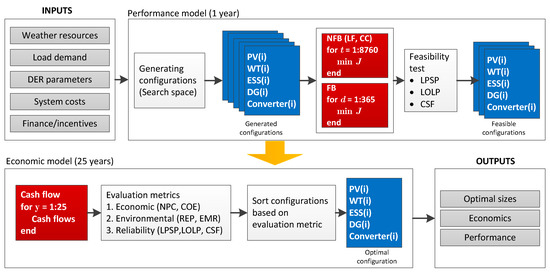
Figure 1.
The simplified architecture of MDSTool. Refer to the nomenclature table for the key to acronyms, variables, and abbreviations in the figure.
3.2. MDSTool Performance Model
In the performance model, various microgrid configurations were generated. The annual operation of each configuration was then simulated using an operating strategy. All of the simulated configurations were then subjected to a feasibility test, using various reliability metrics. The configurations that passed the feasibility test were passed on to the economic model for economic analysis. In the following section, the objective function, operating strategies, and reliability metrics are described.
3.2.1. Objective Function
In the performance model, economic dispatch and unit commitment problem has to be solved to select the combination of DERs which meets the required power at the minimum operating cost while satisfying operation constraints. The operating cost, J, given by Equation (1):
where , , and denote the grid, storage, and generator cost functions, respectively. Note that even though a diesel generator (DG) is used in this study, the generator generally can be an internal combustion generator that burns any type of fuel.
(1) Grid cost function
The grid cost function accounts for the cost of purchasing power from the grid and the revenue obtained from selling power to the grid:
where and are the grid purchase and sale rate in $/kWh, respectively, and and are the grid purchase and sale power in kW, respectively.
(2) Storage cost function
The cost function of ESSs accounts for the degradation and charging costs. The charging cost is the cost of charging the ESS; this can be done by either generator or by purchasing power from the grid. The charging cost is zero if the ESS is charged using renewable energy (PV, WT, etc.) because no additional costs are incurred, unlike charging with a generator or grid, where fuel cost and grid charges applied:
where is the ESS replacement cost in $/kWh, is the ESS throughput in kWh, NESS is the number of ESSs in the ESS bank, is the ESS round-trip efficiency, is the ESS charging cost in $/kWh, is the ESS charge power in kW, and is the ESS discharge power in kW.
(3) Generator cost function
The operating cost of a generator has two parts: fixed costs and variable costs. The fixed cost is the cost per hour of running the generator. The variable cost is the cost per kWh of producing power from the generator. Fixed cost is calculated as shown below:
where is the generator operation and maintenance cost in $/kW/h, is the generator replacement cost in $/kW, is the generator lifetime in hours, q0 is the fuel curve intercept in l/h, is the generator rated power in kW, and is the fuel price in $/l. The variable cost is calculated as shown below:
where q1 is the fuel curve slope in l/h/kW. The generator cost function is then given as the summation of the fixed and variable costs:
Where PGEN is the generator output power in kW.
The objective function in Equation (1) is subject to the following constraints:
- Power balance constraints ensure that the total power produced in the microgrid is equal to the total power consumed.where PLOAD is the load demand, is the output power of DER technologies, both RESs and non-RESs, j is the index of DER technologies. Power loss is assumed to be negligible and therefore not included in the above equation. This assumption is widely adopted in microgrid due to the small size of the distribution network.
- Operation constraints ensure that all DERs operate within their minimum and maximum power, and that grid purchase and sale do not exceed their maximum limits:
- Ramp-up/ramp-down constraints ensure that all DERs do not increase or decrease power beyond their ramp-up/ramp-down limits:
3.2.2. Operating Strategy
The operating strategies can be broadly classified according to whether the forecast is considered or not. They can be non-forecast-based or forecast-based strategies.
(1) Non-forecast based (NFB) strategy
In an NFB strategy, a unit commitment and economic dispatch were solved at each time step of the simulation, without considering future events. The most widely used NFB strategies are load-following (LF) and cycle-charging (CC), developed in [55]. In the LF strategy, the ESS is charged using RES only, unless the generator is operating below its minimum power. The LF strategy can be subcategorized according to how primary control (voltage/frequency control) is achieved. If the ESS and generator control the voltage/frequency by coordinating as a master/slave, then this is termed load-following off (LF-OFF). Whereas if only the generator is used to control the voltage/frequency, then it will always be running, and this is termed load-following on (LF-ON). In the CC strategy, whenever the generator is in operation, it is used to charge the ESS up to a particular state of charge. A comprehensive description of these strategies is available in [55].
(2) Forecast-based (FB) strategy
The FB strategy operates the system by considering future events. This is possible by using a forecast of the load demand, renewable power, and energy prices. If the forecast is assumed to be perfect, then this strategy will result in the most economical operation. However, in practical application, the forecast will not be perfect, and the forecasting errors will reduce the accuracy of the dispatch. In other words, the advantage of the FB operating strategy depends on the accuracy of the forecasting algorithm.
3.2.3. Reliability Metric
The intermittency of RES, along with the fluctuating power demand will affect the power balance of the microgrid; therefore, evaluating microgrid reliability is necessary. The most widely used metric is the loss of power supply probability (LPSP). The LPSP is the probability that an insufficient power supply will result when the microgrid cannot satisfy the load [56]:
Other metrics used to evaluate microgrid reliability include loss-of-load-probability (LOLP) and unmet load. Reference [57] gave the recommended values of these metrics. These reliability metrics are used in the performance model to select feasible configurations.
3.3. MDSTool Economic Model
All of the feasible configurations simulated in the performance model were subjected to an economic analysis by calculating their cash flow throughout the analysis period. An evaluation metric was then used to select the optimal configuration.
3.3.1. Cash Flow
The economic model of MDSTool uses cash flow analysis to calculate the microgrid pre-tax and after-tax cash outflow (expenses) and cash inflow (revenue).
The pre-tax cash outflow is composed of the costs associated with installation, operation and maintenance (O&M), replacement, fuel, electricity charge cost of utilities, insurance, property tax, and emission penalties. The only cash outflow in year zero is the project equity (), defined as a part of an investment that was directly financed with a down payment:
where CINSTALL is the total install cost, and fd is the debt fraction.
The cash outflow for subsequent years includes all expenses incurred during the lifetime of the microgrid. The pre-tax cash outflow () for analysis year n was computed using Equation (14):
where CO&M is the annual operation and maintenance cost, CREP is the replacement cost, CPUR is the annual grid purchased, CFUEL is the annual fuel cost, CINS is annual insurance cost, CPRT is the annual property tax, CEMP is the annual emission penalty, r is the inflation rate, and φ is the escalation rate.
Pre-tax cash inflow in year zero () was equal to investment-based incentive (IBI):
In subsequent years, the pre-tax cash inflow () included all of the microgrid’s revenue as follows:
where CPBI is the production-based incentives, CSALE is the annual revenue from grid sale, and CEMRC is the annual emission reduction credits.
At the end of the analysis period, N, the salvage value was added to the right-hand side of Eq. (12). The total pre-tax cost () was the net difference between pre-tax cash inflow () and cash outflow (FOUT). The total pre-tax cash flow () was the net difference between pre-tax cash inflow and cash outflow, including the value of energy savings (CSAVINGS), as a result of microgrid deployment. The was used to calculate the pre-tax cost metric used for optimal sizing analysis. The was used to calculate pre-tax capital budgeting metrics for the financial feasibility analysis:
3.3.2. Evaluation Metric
Several evaluation metrics can be used to select the optimal configuration. These can be economic, environmental, and/or reliability metrics. The metric used in this study was the LCOE. The LCOE is the ratio of all the costs that occur during the lifetime of the microgrid to the useful energy generated during the lifetime of the microgrid, all discounted to the current year.
4. Case Study
4.1. Descriptions of the Communities
Three remote communities were selected as case studies for the design of remote microgrids, including Cachuela Esperanza, Rosario del Yata, and Villa Bella. All of these communities are located in the Beni Department of Bolivia, near the border with the Republic of Brazil, in the middle of the Amazon. The department contains the most remote dwellings in the country and, therefore, this area is one of the most difficult ones to electrify. In May 2019, the authors visited all three communities to conduct socio-economic surveys, study the existing systems, interview community groups, and meet local authorities. Currently, diesel generators power all of the communities. Table 1 summarizes the basic information obtained from the communities.

Table 1.
Location of the communities.
Cachuela Esperanza is situated on the Beni River, 30 km before its confluence with the Mamoré River. These rivers form the Madeira River there. The population of the community was 800 people living in 150 households, at the time of the investigation. Rosario del Yata is part of the Guayaramerin municipality in the province of Vaca Diez. It has a population of 540 people living in 116 households.
There are 15 commercial buildings and two government buildings in this community. Villa Bella is a small community located in northern Bolivia, near the border with Brazil. It has a total population of 200 people living in 48 households. Among these households, only 28 were connected to the electricity supply. The main economic activities of these communities include fishing, hunting, cattle raising, and agriculture. Figure 2 shows the locations of these communities.
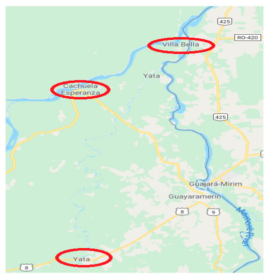
Figure 2.
Location of Cachuela Esperanza, Rosario del Yata, and Villa Bella. Source: Google Maps.
4.2. Electricity Demand Assessment
Detailed electricity demand data are perhaps the most critical data required for hybrid energy system design. However, the data are often unavailable in remote communities. In most cases, a survey is used to create the data, but the accuracy of this method has been questioned by many researchers [58,59]. Therefore, a survey approach was not used in this study. During the site visits, the authors obtained a detailed, hourly load profile of several days of May 2019. The data were complemented with additional information acquired from the local utility company, Empresa Nacional de Electricidad, to create the demand profile for other months. Two additional criteria were considered for creating load profiles: seasonal differences and future load growth. The climate of Bolivia has two seasons, the rainy season and the dry season. The climate is hot and humid, and it is characterized by heavy rainfall caused by winds blowing from the Amazon rainforest. Therefore, the load was scaled to be higher in the rainy and hot season for six months (October to March) and lower in the dry season for the other six months (April to September). The demand during the rainy and hot season was higher than during the dry season, due to the more frequent usage of lighting and fans because of the higher temperatures and humidity. The obtained load profiles show peaks during the early hours of the day, before the start of school and other commercial activities, as well as high demand in the afternoon and another peak toward the end of the day. Future load growth was considered after the initial deployment of the microgrids. This is important because many microgrids report explosive load growth after initial deployment. An example of this includes microgrids on Dongfushan Island, Beiji Island, and Nanji Island, which are all located in the East China Sea [60]. For this reason, the load was scaled up by 25%. Table 2 summarizes the average load, peak load, load factor, and the total annual load of the three communities.
Table 2.
Summary of the electricity demand of the communities.
4.3. Weather Resources Analysis
To estimate the energy production from the solar PV, Global Horizontal Irradiance (GHI) data are required. GHI is the total irradiance from the sun that falls on a horizontal surface on Earth. The data were obtained from the database of NASA Surface Meteorology and Solar Energy [61]. The location of the communities is about 300 meters above sea level, which makes the solar radiation lower in comparison to other regions of Bolivia, which can be as high as 5,000 meters above sea level. The monthly average GHI and clearness index of the region are shown in Figure 3.
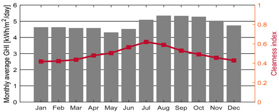
Figure 3.
Monthly average GHI and clearness index.
4.4. DER Technical Parameters
The DER technical parameters were required to conduct performance simulations. The parameters were taken from manufacturer datasheets. The PV module was monocrystalline technology. In selecting the BES technology, factors such as technological maturity, economy, safety, and environmental impacts were considered. Lithium nickel manganese cobalt oxide (NMC) was selected in this study due to its several advantages over other battery chemistries. The NMC batteries have a high rate of discharge, good round-trip efficiency, long lifetime, and a low self-discharge rate. The parameters of all the DER are summarized in Table 3.
Table 3.
Technical parameters of DER technologies.
4.5. DER Costs
The International Renewable Energy Agency (IRENA) has compiled a dataset of solar PV and BES installation costs for commercial and utility-scale projects [62]. The DER costs of this database are used in this study, which is broken down as follows: hardware costs, installation costs, and soft costs. In addition, there are control and monitoring costs, which are estimated to be $100,000 for each microgrid. These costs are summarized in Table 4.
Table 4.
Costs of DER technologies.
4.6. Financial Parameters and Assumption
A discount rate is one of the key parameters in any economic analysis. It is required to discount the future cash flow back to the investment year. Many factors affect the choice of a discount rate, among which are the interest rate, investor’s rate of return, analysis period, and risk premium, among others [63]. IRENA uses 7.5% for the Organization for Economic Cooperation and Development countries and China and 10% for the rest of the world as a real discount rate for evaluating renewable energy investment [64]. Considering that Bolivia is a developing country, a real discount rate of 10% was used in this study. This value is corroborated by the Bolivian Electricity Law, which states that the electricity sector shall use a real discount rate of 10% [65].
5. Results and Discussion
5.1. Cases and Scenarios Definition
Three types of analyses were performed. The first was the base case analysis, presented in Section 5.2. The base case system was simulated using the parameters described in the previous section. The second was a sensitivity analysis, presented in Section 5.3, where the impacts of various policy and technology parameters were investigated. This analysis was performed by keeping the optimal sizes of the DERs in the base case fixed. Therefore, the analysis does not produce other design alternatives, but rather, it shows the impact of varying the selected parameters on the economics of the system (LCOE). Lastly, scenario analyses were presented in Section 5.4. Scenario analysis aims to explore the impacts of the most sensitive policy and technology parameters on configuration, LCOE, REP, and pollutant emissions. Note that the parameters used for scenario analyses were the most sensitive parameters identified in the sensitivity analysis. Therefore, scenario analysis is about producing other design alternatives. For example, it answers questions such as what are the other design alternatives if different discount rates were used. This is important, as it helps to elucidate the sensitive parameters affecting the optimal configuration.
5.2. Base Case Results and Analysis
The results presented in this study for all three communities include optimal sizing, economic summary, and a summary of system performance. The optimal sizing results provided the optimal size of each DER technology in the microgrid: PV, BES, BES inverter, and DG. The economic summary provided results such as LCOE, capital expenditure (CAPEX), and operating expenditure (OPEX). The summary of system performance provided results regarding the technical performance of the system by reporting metrics such as BES lifetime, fuel consumption, and pollutant emissions.
The results of the base cases were tabulated in Table 5, Table 6 and Table 7. The reference case and four microgrid cases were simulated. All of the microgrid base cases were simulated using LF-OFF operating strategies, which is the most common strategy for operating stand-alone microgrid. The reference case was the existing system where all demand was met by using DGs. This case was important because it served as the reference against which the other cases were compared. This case had the lowest CAPEX and highest LCOE and OPEX. The next case was the optimal microgrid system. The optimal system was the microgrid that had the lowest LCOE. In all three communities, the REP of the optimal system was greater than 70%, indicating that high renewable penetration was economically feasible, even though the CAPEX was high. Three more cases were simulated using various REPs of 30%, 50%, and 70%. The results indicated that the increasing REP would increase CAPEX and decrease OPEX in all the communities, as shown in Figure 4. As shown in Figure 5, across the three communities, Cachuela Esperanza had the lowest LCOE, followed by Rosario del Yata and Villa Bella, indicating that the size of the community, and hence the load demand, affected the LCOE. This was expected for two reasons. The first reason is technical, because Cachuela Esperanza had the highest energy demand, it had relatively lower excess energy. The second reason was due to the economy of scale. Since it is the bigger system, its fixed cost per kW was lower, leading to lower LCOE. In general, the results indicated that deploying a microgrid in all three communities was economically feasible.
Table 5.
Results of the baseline cases for Cachuela Esperanza.
Table 6.
Results of the baseline cases for Rosario del Yata.
Table 7.
Results of the baseline cases for Villa Bella.
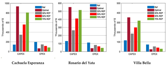
Figure 4.
The capital (CAPEX) and operating (OPEX) expenditures under various REP.
Figure 5.
A plot of REP and LCOE.
5.3. Sensitivity Analysis
In a sensitivity analysis, some selected input parameters are varied over a strategically pre-determined range in order to find which of these parameters results in a greater variation in the output. It is, therefore, possible to use sensitivity analysis to find the parameters that have a significant impact on the economics of the microgrid. In this study, policy and technology parameters were selected for sensitivity analysis. These parameters, shown in Table 8, were strategically chosen based on several factors such as degree of uncertainty and market trends.
Table 8.
Range of the parameters for sensitivity analysis.
Figure 6 shows the results of the sensitivity analyses for the three communities. Generally, as is evident from the figure, some parameters affect the LCOE more than others. In particular, discount rate, diesel price, grants, BES lifetime, and operating strategies have the most significant impact on the LCOE. Sensitivity to the operating reserve and solar irradiance is negligible, meaning these parameters have only a small effect on the LCOE. Sensitivity to fuel type is considerable and exceeds both operating reserve and solar irradiance.
Figure 6.
Variation in LCOE due to the variation of the nine parameters investigated.
5.4. Scenario Analysis
Through sensitivity analyses in the previous section, five parameters were identified as having the greatest impact on the LCOE of the microgrids: discount rate, diesel price, grants, battery lifetime, and operating strategies. Using these parameters, five scenarios were formulated.
5.4.1. Scenario 1: Discount Rate
The base cases in this study were simulated with a real discount rate of 10%. However, the cost of debt and the required return on equity, as well as several other factors, will affect the actual value of the discount rate. Consequently, four scenarios were developed using discount rates of 3%, 5%, 7.5%, and 10%.
Figure 7 shows the results of the cases, indicating that lowering the discount rate results in reducing the LCOE and increasing the REP. This highlights an important policy issue: policies and regulations can be used to minimize the risks for renewable energy investments, therefore, lowering the discount rate, consequently reducing the LCOE. Furthermore, these results suggest that all things being equal, microgrids in developed countries will be more economical and have higher REP than in developing countries. This is because discount rates in developed countries are lower since the cost of borrowing is low and there are regulatory policies that tend to reduce the perceived risk of renewable energy projects. The detailed results of this scenario are tabulated in Appendix A, Table A1.
Figure 7.
The results of Scenario 1 for the three communities: (a) The microgrid configurations under various discount rates; (b) LCOE, REP, and tCO2 under different discount rates. The y-axes are normalized to the base cases. The discount rate applied in each scenario was as follows: Scenario 1A (S1A) was 10%; Scenario 1B (S1B) was 3%; Scenario 1C (S1C) was 5%; Scenario 1D (S1D) was 7.5%.
5.4.2. Scenario 2: Diesel Price
The average diesel price varied considerably across countries. For example, as of 2016, diesel prices were 0.22 $/liter in Iran, 0.65 $/liter in the United States, and 1.63 $/liter in Iceland [68]. Even within a country, several factors affect the price, including pricing framework, sub-national tax, distribution costs (distance between suppliers to end-users), marketing costs, and refining costs (environmental regulations) [69]. At the time of this study, the average pump price of diesel in Bolivia was 0.55 $/liter. However, in remote areas, the average price was 1.41 $/liter. The Bolivian Government subsidizes diesel used for power generation in remote areas to 0.16 $/liter. At the world and regional level, the world’s average pump price was 0.82 $/liter, and the average pump price in Latin America and the Caribbean was 0.74 $/liter. These prices were used to formulate the scenarios in this section.
The results of these scenarios are shown in Figure 8. Both the optimal sizes of PV and BES increased with increasing diesel prices, leading to lower LCOE and signaling that higher prices of diesel would make microgrid investments attractive. This leads to an important policy dilemma because, while subsidizing diesel would force the LCOE to be lower for a diesel-only system, the subsidy would make microgrid investments less attractive, thereby discouraging renewable energy investments in microgrids. As shown in Figure 8, Scenario 2E, with subsidized diesel, diesel-only systems were more attractive, meaning no investments in PV and BES. The detailed results of this scenario are tabulated in Appendix A, Table A2.
Figure 8.
The results of Scenario 2 for the three communities: (a) The microgrid configurations under various diesel prices; (b) LCOE, REP, and tCO2 under different diesel prices. The y-axes are normalized to the base cases. The diesel price applied in each scenario was as follows: Scenario 2A (S2A) was 1.41 $/l; Scenario 2B (S2B) was 0.82 $/l; Scenario 2C (S2C) was 0.74 $/l; Scenario 2D (S2D) was 0.55 $/l; Scenario 2E (S2E) was 0.16 $/l.
5.4.3. Scenario 3: Grants
Renewable energy projects may enjoy some grants/incentives or subsidies from governments, non-governmental organizations, and/or international donor organizations. Therefore, cases were developed where their impacts on the design were developed. Four scenarios were formulated with the grants of 0%, 25%, 50%, 75%, and 100%, and the results are shown in Figure 9.
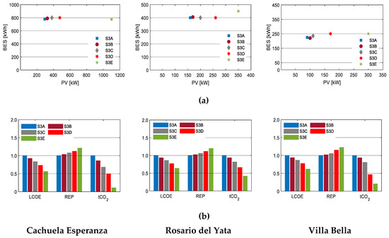
Figure 9.
The results of Scenario 3 for the three communities: (a) The microgrid configurations under various amounts of grants; (b) LCOE, REP, and tCO2 under various amounts of grants. The y-axes are normalized to the base cases. The amount of grants applied in each scenario were as follows: Scenario 3A (S3A) was 0%; Scenario 3B (S3B) was 25%; Scenario 3C (S3C) was 50%; Scenario 3D (S3D) was 75%; Scenario 3E (S3E) was 100%.
Grants can significantly lower the LCOE and increase the REP. It is important to note that, while grants lower the LCOE, they may lead to systems with significantly higher excess renewable energy. The important policy issue here is that, instead of giving more grants to a particular microgrid that may produce excess energy, it would be more efficient from both a cost and an emission reduction perspective to spread the grants to other communities. The detailed results of this scenario are tabulated in Appendix A, Table A3.
5.4.4. Scenario 4: Battery Technology
Other scenarios were produced utilizing other battery technologies: Lithium-ion, lead-acid, and flow batteries. These battery technologies were widely used in hybrid energy systems in remote communities around the world [70]. For example, lithium-ion batteries have been used in the Gasa Island microgrid in South Korea [71], lead-acid batteries have been used in the Beiji Island microgrid in China [72], and flow batteries have been used in Ban Pha Dan microgrid in northern Thailand [73]. Among the three types of battery technologies investigated, each one has its pros and cons. Lithium-ion batteries have a better energy density, a high depth of discharge, higher efficiency, and low self-discharging. However, they are generally more expensive than lead-acid batteries. Conversely, lead-acid batteries are typically cheaper and easier to recycle, but they have a relatively low energy density, a low depth of discharge, and are less efficient. Flow batteries have high upfront investment costs compared to other battery technologies. However, these have a lifetime that typically exceeds 10,000 full cycles, enabling them to make up for the high initial cost.
The following battery chemistries were used to produce the scenarios in this section: lithium nickel manganese cobalt oxide (NMC), lithium iron phosphate (LFP), flooded lead-acid batteries (FLA), valve-regulated lead-acid batteries (VRLA), vanadium redox flow batteries (VRFB), and zinc-bromine flow batteries (ZBFB). The details of the battery parameters were taken from [64] and are summarized in Table 9.
Table 9.
Summary of the properties of various types of batteries.
The results indicate that battery chemistry significantly affects both the optimal sizes of PV and BES, as well as other economic and technical parameters, as shown in Figure 10. For lithium-ion batteries, the results suggest that even within the same technology, the configuration and economics of the systems may differ, based on battery chemistry (NMC and LFP). The ZBFB produced the configuration with the highest LCOE, whereas VRFB led to the lowest LCOE. Overall, the battery technology choice results in relatively flat LCOE, regardless of the chemistry used. The large variation of LCOE in the sensitivity analysis is because only the lifetime is varied, while other properties remained fixed. The implication is more on capital costs, replacement schedules, REP, and pollutant emissions. The detailed results of this scenario are tabulated in Appendix A, Table A4.
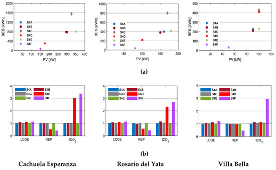
Figure 10.
The results of Scenario 4 for the three communities: (a) The microgrid configurations under various battery technologies; (b) LCOE, REP, and tCO2 under various battery technologies. The y-axes are normalized to the base cases. The battery technology used in each scenario was as follows: Scenario 4A (S4A) was NMC; Scenario 4B (S4B) was LFP; Scenario 4C (S4C) was FLA; Scenario 4D (S4D) was VRLA; Scenario 4E (S4E) was VRFB; Scenario 4F (S4F) was ZBFB.
5.4.5. Scenario 5: Operating Strategy
As described in Section 3, there are four general types of operating strategies that can be used to simulate the operation of a remote microgrid, including LF-OFF, LF-ON, CC, and FB. The base case was simulated using the LF-OFF operating strategy.
As shown in Figure 11, the type of dispatch strategy used to simulate the system affects the configuration, economics, REP, and pollutant emissions. The LF-OFF and FB dispatch strategies consistently had the lowest LCOE and highest REP in all the communities investigated. The FB strategy, which assumed the perfect knowledge of 48 hours of incoming demand of renewable energy, was the most economical. However, the difference between the FB and LF-OFF strategies was negligible. This is consistent with the findings of [55], in which they argued that either CC or LF, whichever was more economical, would be very close to the FB strategy. The LF-OFF strategy allowed for the highest REP because it turned off the diesel generator whenever the PV and BES could meet the load demand. It also utilized BES more efficiently by not charging it with a diesel generator. The LF-ON strategy was the most inefficient and resulted in higher LCOE. This strategy also allowed the least REP because the diesel generator was always running, resulting in higher curtailment of renewable energy. As mentioned previously, the LF-OFF and FB strategies achieved the lowest LCOE and highest REP. However, there was a drawback to these strategies. The switching on and off between BES and the diesel generators led to reliability issues. For this reason, one alternative is to use droop control, which has been proposed in the literature [74]. This method of plug and play makes it possible for all the DER to share power between them, without any communication. The method was successfully tested experimentally and has been applied to some remote communities. However, its widespread adoption has not yet taken place. The detailed results of this scenario are tabulated in Appendix A, Table A5.
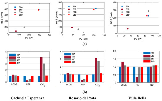
Figure 11.
Results of Scenario 5 for the three communities: (a) The microgrid configurations under various operating strategies; (b) LCOE, REP, and tCO2 under different dispatch strategies. The y-axes are normalized to the base cases. The operating strategy applied in each scenario was as follows: Scenario 5A (S5A) was LF-OFF; Scenario 5B (S5B) was LF-ON; Scenario 5C (S5C) was CC; Scenario 5D (S5D) was FB.
5.5. Discussion
5.5.1. Implications for Policymakers
The study identifies three policy parameters that microgrid investment can be influenced. These parameters include the discount rate, diesel price, and grant. The discount rates in developing countries are relatively high. In Bolivia, for example, the government fixed 10% as a discount rate to be used for evaluating energy projects in the public sector. This value is high, and our results indicate that lowering this value will increase the REP and lower LCOE. For private investment, where governments have no direct control over the discount rates, policymakers can still lower it indirectly by adopting policies that will lower risks associated with renewable energy investment. For fuel prices, there is an existing fuel subsidy in most developing countries. In Bolivia, diesel enjoys a huge subsidy. The subsidy, while helping in improving energy access to remote communities, will make microgrids less economical. These are conflicting objectives that policymakers need to address. Regarding grants, various governments in developing countries offer generous grants for renewable energy projects. This helps in lowering the LCOE of microgrids. However, policymakers need to make a careful evaluation of a better strategy of implementing these grants. For example, instead of subsiding the upfront cost of microgrid, another alternative is to offer grants to people willing to start entrepreneurship activities. This will consequently lower the LCOE of microgrids due to more energy consumption, and at the same time increasing the ability to pay, making the systems to be more sustainable in the long term. The IDCOL initiative in Bangladesh is an example of this approach to giving grants.
5.5.2. Implications for Microgrid Planners
The study identifies two technology parameters that microgrid investment can be influenced. These are battery technology and operating algorithm. Through careful evaluation of battery technologies, the economics of microgrids could be influenced. Our results suggest that LCOE varies slightly for different battery technologies. However, battery technology can be selected to influence the economic behavior of microgrid in a variety of ways. For example, if the upfront cost is the main concern, a battery technology with less capital cost, such as lead-acid types, can be used. On the other hand, frequent replacements can be avoided by selecting battery technology with a longer lifetime. For the operating algorithm, the method adopted will dictate the types of the controller to be used. Controller cost forms a substantial part of upfront cost, therefore, by carefully selecting an appropriate control technique, the economics of microgrid could be influenced by microgrid planners.
6. Conclusions
In this study, the impacts of policy and technology parameter variations on the economics of microgrids for rural electrification were investigated. The investigation was conducted on case studies of three rural communities in the Beni Department of Bolivia using the MDSTool as a modeling tool. The microgrid investment was robust across a wide range of parameters.
It was found that the discount rate, diesel prices, grants, battery technology, and operating strategy, have a significant impact on the configuration, LCOE, REP, and pollutant emission. Remarkably, policymakers and microgrid planners have an influence on these parameters. For policymakers, the implications of this study are threefold. First, making policies that will lower the discount rate can be a useful tool in reducing the LCOE of microgrids, making them more attractive. Second, fuel subsidies, while helping to make electricity more affordable to the rural communities, would discourage investment in microgrids. Third, grants can be used to influence the size of a microgrid, which will consequently make it more economical. For microgrid planners, this study revealed two areas where microgrid investments could be influenced. First, even though different battery technology results in relatively flat LCOE, they can be used to influence capital costs, replacement schedules, REP, and pollutant emissions. Second, the operating strategy will dictate the type of control approach to be adopted, such as centralized, decentralized, or peer-to-peer control. The choice of control will have a significant impact on the cost, reliability, and scalability of the microgrid. In future studies, the authors are interested in investigating the interaction of policy and technology parameters and how they can influence the potential of various microgrid business models for rural electrification.
Author Contributions
Conceptualization, M.H. H.-J.K. and I.-Y.C.; methodology, M.H.; formal analysis, I.-Y.C.; investigation, M.H.; resources, H.-J.K.; writing—original draft preparation, M.H.; writing—review and editing, M.H; supervision, I.-Y.C.; project administration, H.-J.K.; funding acquisition, H.-J.K. All authors have read and agreed to the published version of the manuscript.
Funding
This research was supported by the National Research Foundation of Korea (NRF) grant funded by the Korea government (MSIT)(No. 2019R1A2C1003880) and the Ministry of Science and ICT, Korea, under the ITRC (Information Technology Research Center) support program (IITP-2018-0-01396) supervised by the IITP (Institute for Information & communications Technology Promotion).
Conflicts of Interest
The authors declare no conflict of interest.
Acronyms
| CAPEX | Capital expenditure |
| CC | Cycle-charging |
| BES | Battery energy storage |
| DER | Distributed energy resources |
| DG | Diesel generator |
| EMR | Emission reduction |
| ESS | Energy storage system |
| FLA | Flooded lead-acid battery |
| LCOE | Levelized cost of energy |
| LF | Load-following |
| LF-OFF/ON | Load-following off/on |
| LFP | Lithium iron phosphate |
| LOLP | Loss-of-load-probability |
| LPG | Liquefied petroleum gas |
| LPSP | Loss of power supply probability |
| MILP | Mixed-integer linear programming |
| NMC | Lithium nickel manganese cobalt oxide |
| NFB | Non-forecast based |
| OPEX | Operating expenditure |
| PV | Photovoltaic |
| REP | Renewable energy penetration |
| RES | Renewable energy sources |
| VRFB | Vanadium redox flow batteries |
| VRLA | Valve-regulated lead-acid batteries |
| WT | Wind turbine |
| ZBFB | Zinc bromine flow batteries |
Appendix A
Table A1.
Scenario 1: Discount rate.
Table A1.
Scenario 1: Discount rate.
| Community | Parameters | Ref. System | S1A (10%) | S1B (3%) | S1C (5%) | S1D (7.5%) |
|---|---|---|---|---|---|---|
| Cachuela Esperanza | PV (kW) | - | 295 | 375 | 350 | 325 |
| BES (kWh) | - | 780 | 850 | 850 | 825 | |
| REP (%) | 0 | 80.5 | 87.7 | 86.4 | 84.3 | |
| LCOE ($/kWh) | 0.506 | 0.398 | 0.275 | 0.309 | 0.354 | |
| Emission (ton/y) | 315.7 | 63.6 | 39.8 | 44.2 | 51.2 | |
| Rosario del Yata | PV (kW) | - | 160 | 200 | 180 | 165 |
| BES (kWh) | - | 400 | 525 | 475 | 415 | |
| REP (%) | 0 | 74.6 | 83.9 | 80.4 | 76.0 | |
| LCOE ($/kWh) | 0.543 | 0.431 | 0.302 | 0.338 | 0.384 | |
| Emission (tCO2/y) | 175.2 | 44.6 | 28.2 | 34.3 | 42.1 | |
| Villa Bella | PV (kW) | - | 90 | 110 | 100 | 95 |
| BES (kWh) | - | 225 | 300 | 275 | 250 | |
| REP (%) | 0 | 78.1 | 86.3 | 83.5 | 81.1 | |
| LCOE ($/kWh) | 0.690 | 0.501 | 0.340 | 0.384 | 0.442 | |
| Emission (ton/y) | 116.3 | 26.0 | 16.2 | 19.5 | 22.4 |
Table A2.
Scenario 2: Diesel prices.
Table A2.
Scenario 2: Diesel prices.
| Community | Parameters | Ref. System | S2A (1.41 $/l) | S2B (0.82 $/l) | S2C (0.74 $/l) | S2D (0.55 $/l) | S2E (0.16 $/l) |
|---|---|---|---|---|---|---|---|
| Cachuela Esperanza | PV (kW) | - | 295 | 110 | 110 | 100 | - |
| BES (kWh) | - | 780 | 110 | 110 | 110 | - | |
| REP (%) | 0 | 80.5 | 32.6 | 32.6 | 30.9 | 0 | |
| LCOE ($/kWh) | 0.506 | 0.398 | 0.317 | 0.301 | 0.263 | 0.144 | |
| Emission (ton/y) | 315.7 | 63.6 | 216.6 | 216.6 | 222.5 | 315.7 | |
| Rosario del Yata | PV (kW) | - | 160 | 55 | 55 | 50 | - |
| BES (kWh) | - | 400 | 40 | 40 | 40 | - | |
| REP (%) | 0 | 74.6 | 27.4 | 27.4 | 26 | 0 | |
| LCOE ($/kWh) | 0.543 | 0.431 | 0.351 | 0.334 | 0.295 | 0.187 | |
| Emission (tCO2/y) | 175.2 | 44.6 | 127.2 | 127.2 | 129.7 | 175.2 | |
| Villa Bella | PV (kW) | - | 90 | 40 | 40 | 30 | - |
| BES (kWh) | - | 225 | 40 | 40 | 40 | - | |
| REP (%) | 0 | 78.1 | 35.7 | 35.7 | 30.9 | 0 | |
| LCOE ($/kWh) | 0.690 | 0.501 | 0.437 | 0.418 | 0.371 | 0.238 | |
| Emission (ton/y) | 116.3 | 26.0 | 76.1 | 76.1 | 81.5 | 116.3 |
Table A3.
Scenario 3: Grants.
Table A3.
Scenario 3: Grants.
| Community | Parameters | Ref. System | S3A (0%) | S3B (25%) | S3C (50%) | S3D (75%) | S3E (100%) |
|---|---|---|---|---|---|---|---|
| Cachuela Esperanza | PV (kW) | - | 295 | 325 | 380 | 475 | 1100 |
| BES (kWh) | - | 780 | 790 | 800 | 800 | 775 | |
| REP (%) | 0 | 80.5 | 83.3 | 86.7 | 90.3 | 97.5 | |
| LCOE ($/kWh) | 0.506 | 0.398 | 0.368 | 0.333 | 0.291 | 0.223 | |
| Emission (ton/y) | 315.7 | 63.6 | 54.7 | 43.4 | 31.5 | 7.0 | |
| Rosario del Yata | PV (kW) | - | 160 | 170 | 200 | 260 | 350 |
| BES (kWh) | - | 400 | 405 | 400 | 400 | 450 | |
| REP (%) | 0 | 74.6 | 76.2 | 79.2 | 83.1 | 89.4 | |
| LCOE ($/kWh) | 0.543 | 0.431 | 0.403 | 0.371 | 0.332 | 0.275 | |
| Emission (tCO2/y) | 175.2 | 44.6 | 41.7 | 36.5 | 29.6 | 18.7 | |
| Villa Bella | PV (kW) | - | 90 | 100 | 110 | 170 | 300 |
| BES (kWh) | - | 225 | 220 | 235 | 250 | 250 | |
| REP (%) | 0 | 78.1 | 79.5 | 82.4 | 89.9 | 95.5 | |
| LCOE ($/kWh) | 0.690 | 0.501 | 0.470 | 0.434 | 0.388 | 0.311 | |
| Emission (ton/y) | 116.3 | 26.0 | 24.3 | 21.0 | 12.1 | 5.4 |
Table A4.
Scenario 4: Battery technology.
Table A4.
Scenario 4: Battery technology.
| Community | Parameters | Ref. System | S4A NMC | S4B LFP | S4C FLA | S4D VRLA | S4E VRFB | S4F ZBFB |
|---|---|---|---|---|---|---|---|---|
| Cachuela Esperanza | PV (kW) | - | 295 | 300 | 325 | 175 | 350 | 150 |
| BES (kWh) | - | 780 | 775 | 1550 | 300 | 800 | 60 | |
| REP (%) | 0 | 80.5 | 80.1 | 80.2 | 40.7 | 80.9 | 33.6 | |
| LCOE ($/kWh) | 0.506 | 0.398 | 0.429 | 0.405 | 0.438 | 0.391 | 0.446 | |
| Emission (ton/y) | 315.7 | 63.6 | 65.1 | 64.9 | 190.8 | 62.6 | 213.7 | |
| Rosario del Yata | PV (kW) | - | 160 | 150 | 170 | 100 | 180 | 80 |
| BES (kWh) | - | 400 | 380 | 800 | 220 | 420 | 40 | |
| REP (%) | 0 | 74.6 | 71.2 | 73.5 | 41.1 | 74.1 | 31.5 | |
| LCOE ($/kWh) | 0.543 | 0.431 | 0.458 | 0.437 | 0.473 | 0.425 | 0.483 | |
| Emission (tCO2/y) | 175.2 | 44.6 | 50.5 | 46.4 | 103.3 | 45.5 | 120.1 | |
| Villa Bella | PV (kW) | - | 90 | 90 | 100 | 100 | 100 | 50 |
| BES (kWh) | - | 225 | 210 | 430 | 410 | 230 | 30 | |
| REP (%) | 0 | 78.1 | 75.8 | 77.3 | 75.7 | 76.6 | 35.6 | |
| LCOE ($/kWh) | 0.690 | 0.501 | 0.530 | 0.507 | 0.555 | 0.495 | 0.598 | |
| Emission (ton/y) | 116.3 | 26.0 | 28.8 | 27.0 | 29.0 | 27.9 | 76.1 |
Table A5.
Scenario 5: Operating strategy.
Table A5.
Scenario 5: Operating strategy.
| Community | Parameters | Ref. System | S5A LF-OFF | S5B LF-ON | S5C CC | S5D FB |
|---|---|---|---|---|---|---|
| Cachuela Esperanza | PV (kW) | - | 295 | 70 | 150 | 290 |
| BES (kWh) | - | 780 | 50 | 185 | 775 | |
| REP (%) | 0 | 80.5 | 20.0 | 37.1 | 79.3 | |
| LCOE ($/kWh) | 0.506 | 0.398 | 0.473 | 0.421 | 0.398 | |
| Emission (ton/y) | 315.7 | 63.6 | 259.2 | 192.7 | 66.0 | |
| Rosario del Yata | PV (kW) | - | 160 | 45 | 75 | 150 |
| BES (kWh) | - | 400 | 90 | 60 | 385 | |
| REP (%) | 0 | 74.6 | 21.3 | 30.5 | 71.2 | |
| LCOE ($/kWh) | 0.543 | 0.431 | 0.521 | 0.467 | 0.431 | |
| Emission (tCO2/y) | 175.2 | 44.6 | 138.1 | 121.5 | 50.4 | |
| Villa Bella | PV (kW) | - | 90 | 30 | 90 | 85 |
| BES (kWh) | - | 225 | 60 | 285 | 225 | |
| REP (%) | 0 | 78.1 | 26.1 | 74.5 | 75.8 | |
| LCOE ($/kWh) | 0.690 | 0.501 | 0.655 | 0.538 | 0.501 | |
| Emission (ton/y) | 116.3 | 26.0 | 26.1 | 27.9 | 28.0 |
References
- Riva, F.; Ahlborg, H.; Hartvigsson, E.; Pachauri, S.; Colombo, E. Electricity access and rural development: Review of complex socio-economic dynamics and causal diagrams for more appropriate energy modelling. Energy Sustain. Dev. 2018, 43, 203–223. [Google Scholar] [CrossRef]
- Kooijman-van Dijk, A.L.; Clancy, J. Impacts of Electricity Access to Rural Enterprises in Bolivia, Tanzania and Vietnam. Energy Sustain. Dev. 2010, 14, 14–21. [Google Scholar] [CrossRef]
- Gibson, J.; Olivia, S. The effect of infrastructure access and quality on non-farm enterprises in rural indonesia. World Dev. 2010, 38, 717–726. [Google Scholar] [CrossRef]
- Wamukonya, N.; Davis, M. Socio-economic impacts of rural electrification in Namibia: Comparisons between grid, solar and unelectrified households. Energy Sustain. Dev. 2001, 5, 5–13. [Google Scholar] [CrossRef]
- WHO. Household air pollution and health. World Health Organisation Factsheet; WHO: Geneva, Swzitzerland, 2016. [Google Scholar]
- Spalding-Fecher, R. Health benefits of electrification in developing countries: A quantitative assessment in South Africa. Energy Sustain. Dev. 2005, 9, 53–62. [Google Scholar] [CrossRef]
- Grogan, L.; Sadanand, A. Rural electrification and employment in poor countries: Evidence from Nicaragua. World Dev. 2013, 43, 252–265. [Google Scholar] [CrossRef]
- Khandker, S.R.; Barnes, D.F.; Samad, H.A. Welfare impacts of rural electrification: A panel data analysis from Vietnam. Econ. Dev. Cult. Chang. 2013, 61, 659–692. [Google Scholar] [CrossRef]
- Dinkelman, T. The effects of rural electrification on employment: New evidence from South Africa. Am. Econ. Rev. 2011, 101, 3078–3108. [Google Scholar] [CrossRef]
- Gustavsson, M. Educational benefits from solar technology—Access to solar electric services and changes in children’s study routines, experiences from eastern province Zambia. Energy Policy 2007, 35, 1292–1299. [Google Scholar] [CrossRef]
- Jacobson, A. Connective power: Solar electrification and social change in Kenya. World Dev. 2007, 35, 144–162. [Google Scholar] [CrossRef]
- WBG. State of Electricity Access Report; WBG: Washington, DC, USA, 2017. [Google Scholar]
- WBG. Tracking SDG7: The Energy Progress Report; WBG: Washington, DC, USA, 2018. [Google Scholar]
- IEA. Energy Access Outlook 2017: World Energy Outlook Special Report; OECD/IEA: Paris, France, 2017. [Google Scholar]
- Mandelli, S.; Barbier1, J.; Mereu, R.; Colombo, E. Off-grid systems for rural electrification in developing countries: Definition, classification and comprehensive literature review. Renew. Sustain. Energy Rev. 2016, 58, 1621–1646. [Google Scholar] [CrossRef]
- Hatziargyriou, N. Microgrids: Architecture and Control; Wiley-IEEE Press: Piscataway, NJ, USA, 2013. [Google Scholar]
- Williams, N.J.; Jaramillo, P.; Taneja, J.; Ustun, T.S. Enabling private sector investment in microgrid-based rural electrification in developing countries: A review. Renew. Sustain. Energy Rev. 2015, 52, 1268–1281. [Google Scholar] [CrossRef]
- WBG. Lighting Africa. Available online: https://www.lightingafrica.org/ (accessed on 23 November 2019).
- Slough, T.; Urpelainen, J.; Yang, J. Light for all? Evaluating Brazil’s rural electrification progress, 2000–2010. Energy Policy 2015, 86, 315–327. [Google Scholar] [CrossRef]
- Mollik, S.; Rashid, M.M.; Hasanuzzaman, M.; Karim, M.E.; Hosenuzzaman, M. Prospects, progress, policies, and effects of rural electrification in Bangladesh. Renew. Sustain. Energy Rev. 2016, 65, 553–567. [Google Scholar] [CrossRef]
- IDCOL. IDCOL SHS Installation under RE Program. Available online: http://www.idcol.org/old/bd-map/bangladesh_map/ (accessed on 1 November 2019).
- Almeshqab, F.; Ustun, T.S. Lessons learned from rural electrification initiatives in developing countries: Insights for technical, social, financial and public policy aspects. Renew. Sustain. Energy Rev. 2019, 102, 35–53. [Google Scholar] [CrossRef]
- Husein, M.; Chung, I.-Y. Optimal design and financial feasibility of a university campus microgrid considering renewable energy incentives. Appl. Energy 2018, 225, 273–289. [Google Scholar] [CrossRef]
- Ho, W.S.; Hashim, H.; Lim, J.S. Integrated biomass and solar town concept for a smart eco-village in Iskandar Malaysia (IM). Renew. Energy 2014, 69, 190–201. [Google Scholar] [CrossRef]
- Ranaboldo, M.; Lega, B.D.; Ferrenbach, D.V.; Ferrer-Marti, L.; Moreno, R.P.; Garcia-Villoria, A. Renewable energy projects to electrify rural communities in Cape Verde. Appl. Energy 2014, 118, 280–291. [Google Scholar] [CrossRef]
- Gupta, A.; Saini, R.P.; Sharma, M.P. Steady-state modelling of hybrid energy system for off grid electrification of cluster of villages. Renew. Energy 2010, 35, 520–535. [Google Scholar] [CrossRef]
- Malheiro, A.; Castro, P.M.; Lima, R.M.; Estanqueiro, A. Integrated sizing and scheduling of wind/PV/diesel/battery isolated systems. Renew. Energy 2015, 83, 646–657. [Google Scholar] [CrossRef]
- Ferrer-Marti, L.; Domenech, B.; Garcia-Villoria, A.; Pastor, R. A MILP model to design hybrid wind–photovoltaic isolated rural electrification projects in developing countries. Eur. J. Oper. Res. 2013, 226, 293–300. [Google Scholar] [CrossRef]
- Kolhe, M.L.; Ranaweera, K.M.I.U.; Gunawardana, A.G.B.S. Techno-economic sizing of off-grid hybrid renewable energy system for rural electrification in Sri Lanka. Sustain. Energy Technol. Assess. 2015, 11, 53–64. [Google Scholar] [CrossRef]
- Akella, A.K.; Sharma, M.P.; Saini, R.P. Optimum utilization of renewable energy sources in a remote area. Renew. Sustain. Energy Rev. 2007, 11, 894–908. [Google Scholar] [CrossRef]
- Nfah, E.M.; Ngundam, J.M.; Vandenbergh, M.; Schmid, J. Simulation of off-grid generation options for remote villages in Cameroon. Renew. Energy 2008, 33, 1064–1072. [Google Scholar] [CrossRef]
- Diaz, P.; Pena, R.; Munoz, J.; Arias, C.A.; Sandoval, D. Field analysis of solar PV-based collective systems for rural electrification. Energy 2011, 36, 2509–2516. [Google Scholar] [CrossRef]
- Bhatt, A.; Sharma, M.P.; Saini, R.P. Feasibility and sensitivity analysis of an off-grid micro hydro–photovoltaic–biomass and biogas–diesel–battery hybrid energy system for a remote area in Uttarakhand state, India. Renew. Sustain. Energy Rev. 2016, 61, 53–69. [Google Scholar] [CrossRef]
- Singh, S.; Singh, M.; Kaushik, S.C. Feasibility study of an islanded microgrid in rural area consisting of PV, wind, biomass and battery energy storage system. Energy Convers. Manag. 2016, 128, 178–190. [Google Scholar] [CrossRef]
- Rehman, S.; Al-Hadhrami, L.M. Study of a solar PV–diesel–battery hybrid power system for a remotely located population near Rafha, Saudi Arabia. Energy 2010, 35, 4986–4995. [Google Scholar] [CrossRef]
- Maleki, A.; Pourfayaz, F. Optimal sizing of autonomous hybrid photovoltaic/wind/battery power system with LPSP technology by using evolutionary algorithms. Sol. Energy 2015, 115, 471–483. [Google Scholar] [CrossRef]
- Blum, N.U.; Wakeling, R.S.; Schmidt, T.S. Rural electrification through village grids—Assessing the cost competitiveness of isolated renewable energy technologies in Indonesia. Renew. Sustain. Energy Rev. 2013, 22, 482–496. [Google Scholar] [CrossRef]
- Bhandari, B.; Lee, K.-T.; Lee, C.S.; Song, C.-K.; Maskey, R.K.; Ahn, S.-H. A novel off-grid hybrid power system comprised of solar photovoltaic, wind, and hydro energy sources. Appl. Energy 2014, 133, 236–242. [Google Scholar] [CrossRef]
- Silva, S.B.; Severino, M.M.; Oliveira, M.A.G. A stand-alone hybrid photovoltaic, fuel cell and battery system: A case study of Tocantins, Brazil. Renew. Energy 2013, 57, 384–389. [Google Scholar] [CrossRef]
- Bilal, B.O.; Sambou, V.; Ndiaye, P.A.; Kebe, C.M.F.; Ndongo, M. Optimal design of a hybrid solar–wind-battery system using the minimization of the annualized cost system and the minimization of the loss of power supply probability (LPSP). Renew. Energy 2010, 35, 2388–2390. [Google Scholar] [CrossRef]
- Belfkira, R.; Zhang, L.; Barakat, G. Optimal sizing study of hybrid wind/PV/diesel power generation unit. Sol. Energy 2011, 85, 100–110. [Google Scholar] [CrossRef]
- Lhendup, T. Rural electrification in Bhutan and a methodology for evaluation of distributed generation system as an alternative option for rural electrification. Energy Sustain. Dev. 2008, 12, 13–24. [Google Scholar] [CrossRef]
- Solano-Peralta, M.; Moner-Girona, M.; van Sark, W.G.J.H.M.; Vallve, X. “Tropicalisation” of Feed-in Tariffs: A custom-made support scheme for hybrid PV/diesel systems in isolated regions. Renew. Sustain. Energy Rev. 2009, 13, 2279–2294. [Google Scholar] [CrossRef]
- Khelif, A.; Talha, A.; Belhamel, M.; Arab, A.H. Feasibility study of hybrid Diesel–PV power plants in the southern of Algeria: Case study on AFRA power plant. Int. J. Electr. Power Energy Syst. 2012, 43, 546–553. [Google Scholar] [CrossRef]
- Zhang, X.; Tan, S.-C.; Li, G.; Li, J.; Feng, Z. Components sizing of hybrid energy systems via the optimization of power dispatch simulations. Energy 2013, 52, 165–172. [Google Scholar] [CrossRef]
- Rohani, G.; Nour, M. Techno-economical analysis of stand-alone hybrid renewable power system for Ras Musherib in United Arab Emirates. Energy 2014, 64, 828–841. [Google Scholar] [CrossRef]
- Domenech, B.; Ferrer-Marti, L.; Lillo, P.; Pastor, R.; Chiroque, J. A community electrification project: Combination of microgrids and household systems fed by wind, PV or micro-hydro energies according to micro-scale resource evaluation and social constraints. Energy Sustain. Dev. 2014, 23, 275–285. [Google Scholar] [CrossRef]
- Ghaib, K.; Ben-Fares, F.-Z. A design methodology of stand-alone photovoltaic power systems for rural electrification. Energy Convers. Manag. 2017, 148, 1127–1141. [Google Scholar] [CrossRef]
- Mandelli, S.; Brivio, C.; Colombo, E.; Merlo, M. A sizing methodology based on Levelized Cost of Supplied and Lost Energy for off-grid rural electrification systems. Renew. Energy 2016, 89, 475–488. [Google Scholar] [CrossRef]
- Adaramola, M.S.; Paul, S.S.; Oyewola, O.M. Assessment of decentralized hybrid PV solar-diesel power system for applications in Northern part of Nigeria. Energy Sustain. Dev. 2014, 19, 72–82. [Google Scholar] [CrossRef]
- Adaramola, M.S.; Agelin-Chaab, M.; Paul, S.S. Analysis of hybrid energy systems for application in southern Ghana. Energy Convers. Manag. 2014, 88, 284–295. [Google Scholar] [CrossRef]
- Mondal, A.H.; Denich, M. Hybrid systems for decentralized power generation in Bangladesh. Energy Sustain. Dev. 2010, 14, 48–55. [Google Scholar] [CrossRef]
- Roy, A.; Kabir, M.A. Relative life cycle economic analysis of stand-alone solar PV and fossil fuel powered systems in Bangladesh with regard to load demand and market controlling factors. Renew. Sustain. Energy Rev. 2012, 16, 4629–4637. [Google Scholar] [CrossRef]
- Bekele, G.; Palm, B. Feasibility study for a standalone solar–wind-based hybrid energy system for application in Ethiopia. Appl. Energy 2010, 87, 487–495. [Google Scholar] [CrossRef]
- Barley, C.D.; Winn, C.B. Optimal dispatch strategy in remote hybrid power systems. Sol. Energy 1996, 58, 165–179. [Google Scholar] [CrossRef]
- Kaldellis, J.K. Stand-Alone and Hybrid Wind Energy Systems; CRC Press: Boca Raton, FL, USA, 2010. [Google Scholar]
- Lorenzo, E. Solar Electricity: Engineering of Photovoltaic Systems; Progensa: SeviIle, Spain, 1994. [Google Scholar]
- Blodgett, C.; Dauenhauer, P.; Louie, H.; Kickham, L. Accuracy of energy-use surveys in predicting rural mini-grid user consumption. Energy Sustain. Dev. 2017, 41, 88–105. [Google Scholar] [CrossRef]
- Hartvigsson, E.; Ahlgren, E.O. Comparison of load profiles in a mini-grid: Assessment of performance metrics using measured and interview-based data. Energy Sustain. Dev. 2018, 43, 186–195. [Google Scholar] [CrossRef]
- Zhao, B.; Zhang, X.; Li, P.; Wang, K.; Xue, M.; Wang, C. Optimal sizing, operating strategy and operational experience of a stand-alone microgrid on Dongfushan Island. Appl. Energy 2014, 113, 1656–1666. [Google Scholar] [CrossRef]
- NASA. Surface Meteorology and Solar Energy. Available online: https://eosweb.larc.nasa.gov/sse (accessed on 5 July 2017).
- IRENA. Renewable Power Generation Costs in 2017; IRENA: Abu Dhabi, United Arab Emirates, 2018. [Google Scholar]
- Short, W.; Packey, D.J.; Holt, T. A Manual for Economic Evaluation of Energy Efficiency and Renewable Energy Technologies; National Renewable Energy Laboratory: Golden, CO, USA, 1995. [Google Scholar]
- IRENA. Electricity Storage and Renewables: Costs and Markets to 2030; IRENA: Abu Dhabi, United Arab Emirates, 2017. [Google Scholar]
- Plurinational State of Bolivia. Reglamento de Precios y Tarifas de la Ley Nº 1604, 28 de Junio de 1995. Available online: https://www.lexivox.org/norms/BO-RE-DS24043D.xhtml (accessed on 16 August 2019).
- Colombo, E.; Riva, F.; Ballon, S. Micro-Grid Optimization for Remanso Village and Evaluation of Possible Off-Grid Configurations for Rural Areas of Bolivia; Politecnico Milano: Milano, Italy, 2018. [Google Scholar]
- Marcos, J.; Marroyo, L.; Lorenzo, E.; Alvira, D.; Izco, E. Power output fluctuations in large scale PV plants: One year observations with one second resolutions and derived analytic model. Prog. Photovolt. Res. Res. Appl. 2010, 19, 218–227. [Google Scholar] [CrossRef]
- WB. Pump Price for Diesel Fuel. Available online: https://data.worldbank.org/indicator/ep.pmp.desl.cd (accessed on 4 November 2019).
- IEA. World Energy Prices. Available online: https://www.iea.org/statistics/prices/ (accessed on 4 November 2019).
- IRENA. Battery Storage for Renewables: Market Status and Technology Outlook; IRENA: Abu Dhabi, United Arab Emirates, 2015. [Google Scholar]
- Husein, M.A.; Vu, B.H.; Chung, I.Y.; Chae, W.K.; Lee, H.J. Design and dynamic performance analysis of a stand-alone microgrid—A case study of Gasa Island, South Korea. J. Electr. Eng. Technol. 2017, 12, 1777–1788. [Google Scholar]
- Zhao, B.; Chen, J.; Zhang, L.; Zhang, X.; Qin, R.; Lin, X. Three representative island microgrids in the East China Sea: Key technologies and experiences. Renew. Sustain. Energy Rev. 2018, 96, 262–274. [Google Scholar] [CrossRef]
- RedFlow. Redflow Batteries Supply Energy for Remote Thai Village. Available online: https://redflow.com/redflow-batteries-supply-energy-for-remote-thai-village/ (accessed on 22 October 2019).
- Bidram, A.; Davoudi, A. Hierarchical Structure of Microgrids Control System. IEEE Trans. Smart Grid 2012, 3, 1963–1976. [Google Scholar] [CrossRef]


© 2020 by the authors. Licensee MDPI, Basel, Switzerland. This article is an open access article distributed under the terms and conditions of the Creative Commons Attribution (CC BY) license (http://creativecommons.org/licenses/by/4.0/).