In this section, the detection algorithms of the DC signals are proposed, including VMD and HT algorithms. Firstly, the principle of VMD algorithm is analyzed in detail, where the complex DC signals can be decomposed into K modes. Next, the HT algorithm is utilized to obtain the instantaneous amplitude, frequency and start-stop time of each mode. Finally, the selection of preset decomposition scale K is also presented.
3.1. Variational Mode Decomposition
In general, the VMD algorithm is an adaptive, quasi-orthogonal and completely non-recursive decomposition method, consisting of classical Wiener Filtering, Hilbert Transform and frequency mixing. It decomposes the input signals composed of multi-components into several inherent modes with limited bandwidth, and most of these modes are closely around their corresponding central frequencies, which meet the definition of intrinsic mode functions (IMFs) [
31].
Unlike the cyclic sieving decomposition used by EMD algorithm, the VMD algorithm transfers the signal decomposition process to the variational framework and achieves adaptive signal decomposition by searching the optimal solution of the constrained variational model. By solving the variational model iteratively, the adaptive decomposition of the signal frequency band can be completed according to the frequency domain characteristics of the decomposed signal, and several band-limited intrinsic mode functions (BLIMFs) components can be obtained, where the sum of estimated bandwidth of each BLIMFs is the smallest and equals to the decomposed signal [
36]. For the original signal
f, the corresponding constrained variational model expression [
31] is
where
represents the
k-th mode component obtained by decomposition,
represents the corresponding central frequencies of the
k-th mode component,
represents the square of norm-2. The first expression of Equation (5) is the optimization objective, and “s.t.” is the abbreviation of “subject to”, which means the constraints of the related optimization problem.
To obtain the optimal solution of the constrained variational problem, an augmented Lagrange function is introduced to transform the constrained variational problem into a non-constrained variational problem [
31], which can be expressed as follows:
where
α represents the quadratic penalty factor, which can guarantee the accuracy of signal reconstruction in the presence of Gauss noise, and
λ represents the Lagrange operator, which can be used to maintain the strictness of constraints. The first term of the augmented Lagrange function represents the quadratic penalty term, and the last one is the Lagrangian multipliers term.
To seek for the optimal solution of the constrained variational problem (the saddle point of the augmented Lagrange function), the alternating direction multiplier method (ADMM) is utilized. By calculation, the expression of
can be given as follows:
where X represents all desirable sets of
. The Equation (7) can be transformed into the frequency domain by utilizing the Parseval/Plancherel Fourier equidistant transformation, it will lead to
where
,
represents the Fourier transformation of signal
,
is random frequency.
In the reconstructed approximation term, the conjugate symmetry characteristics of real signals can be used to transform Equation (8) into a half-space integral form of non-negative frequencies, which can be obtained as,
For positive frequencies, it is easy to get the solution of this quadratic optimization problem if making
as follows:
From (10), can be equivalent to the Wiener filter of the current residual signal, and the full spectrum of the real mode can be obtained by conjugate symmetry. Thus, the real part can be achieved through utilizing the inverse Fourier transform of .
Similarly, to obtain the minimum value of
, the central frequency updating problem can be transformed into the corresponding frequency domain, which can be expressed as follows,
By calculations, the solutions of the central frequencies can be given,
Therefore, the new value of can be set to the center of gravity of the corresponding modal power spectrum.
To update the Lagrange operator
λ [
31], the following expression is given,
where
τ represent Lagrange multipliers updating parameters.
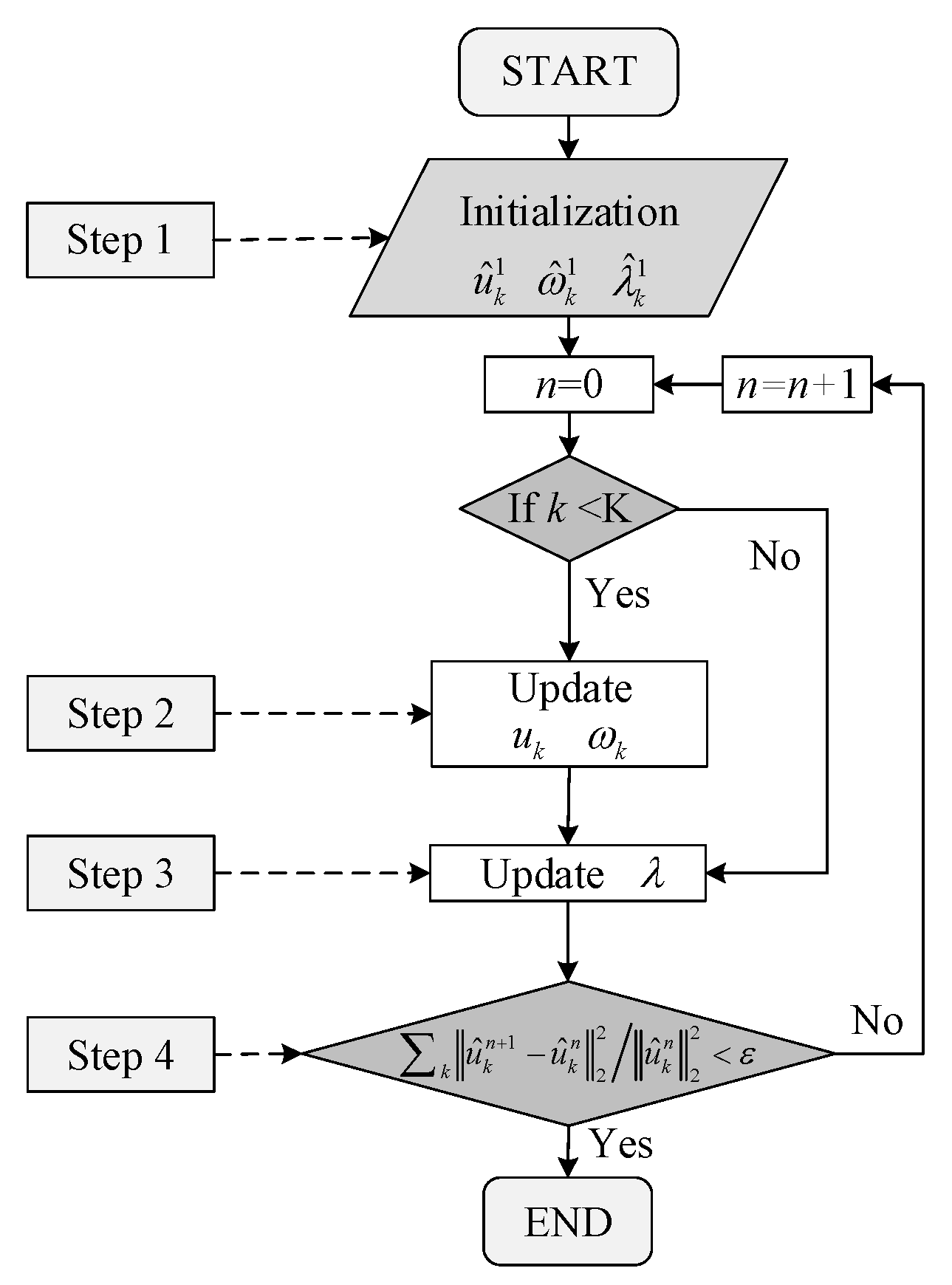
According to the above analysis, the detailed procedures of VMD algorithm are given as follows.
(1) Initialize parameters , and ;
(2) Update and according to Equations (10) and (12);
(3) Update λ according to Equation (13);
(4) Set the error , If the inequality () holds, then the iteration stops, else go back to step (2).
According to the above analysis, a finite number of IMFs
with specific sparsity properties can be obtained non-recursively. The VMD algorithm is more robust to noise, because wiener filter is embedded to update the modes. Flow chart for solution of VMD is shown in
Figure 1.
3.2. Hilbert Transform
Firstly, the preset decomposition scale K of input signals should be determined through utilizing the Fourier transformation. Then, the PQ disturbance signals can be decomposed into the sum of a series of mode functions with VMD algorithm, and each mode is a FM and AM function. Finally, the instantaneous amplitude and frequency of the corresponding modes are obtained by Hilbert demodulation. The specific steps can be given as follows.
(1) Determine the preset decomposition scale K of input signals.
(2) Decompose
into K modes, which can be expressed as follows:
(3) Obtain the corresponding instantaneous amplitude
and frequency
of mode
through utilizing the Hilbert transformation.
The corresponding analytical signal can be given by
Define
as the phase function of
, then it will lead to
The instantaneous frequency
of mode
can be obtained through gaining the derivation of phase function
.
As shown in
Figure 2, the instantaneous amplitude, frequency and start-stop time of disturbance signal will be detected by utilizing the VMD and HT algorithms.
3.3. The Selection of Preset Decomposition Scale K
Before processing the DC signals with VMD-HT algorithm, the optimal modal number K should be determined in advance. Whether the set of modal components is reasonable directly affects the final decomposition results. If the presupposed K value is less than the number of useful components in the processed signal, it will cause inadequate decomposition, so that some BLIMFs cannot be decomposed; if the presupposed K value is larger than the number of useful components in the processed signal, it will cause excessive decomposition, resulting in some useless false components, interfering with the original signal. Once the modal number K is known, the detection of the amplitudes and frequencies of these mode components becomes easier and more accurate. Therefore, the determination of mode number K plays an important role in VMD-HT algorithm.
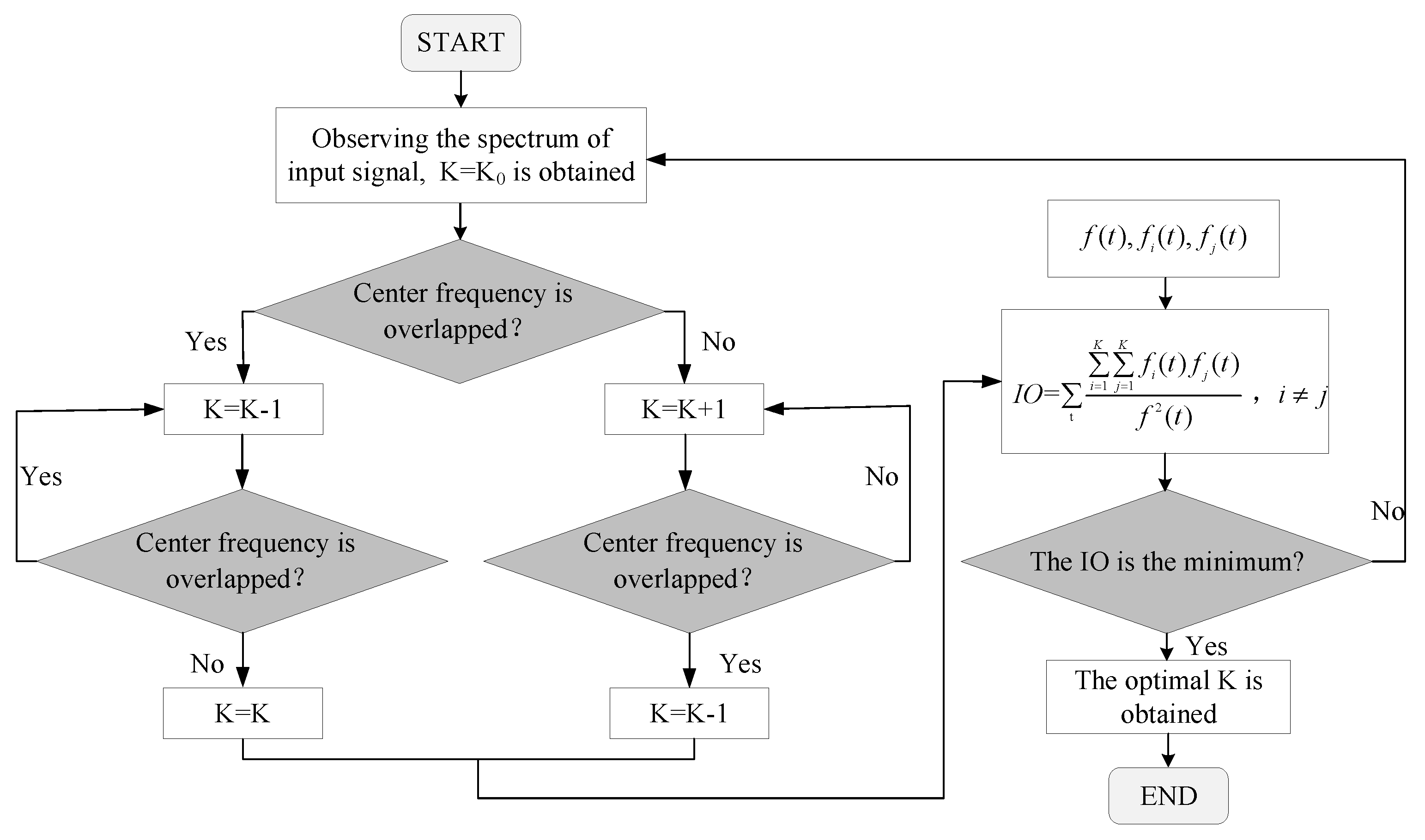
As reported in [
31,
32], the optimal mode number K can be chosen mainly through observing the central frequencies of the decomposed modes, and then the correctness of the selected K can be determined by using the orthogonal index (IO) [
27], which is defined as,
where
is the input signal,
and
are the
i and
j modes, respectively. IO denotes the degree of orthogonality between all modes.
The flowchart of mode number determination is shown in
Figure 3. For the VMD-HT algorithm, the different values of K correspond to different IO. The mode number K is initially determined by observing the central frequencies of the decomposed modes. When IO is the minimum value, that is, whether K decreases or increases, IO will increase, then the corresponding K value is optimal, and the VMD-HT algorithm has the highest decomposition accuracy at the moment. Therefore, combined with the observation of central frequencies of the decomposed modes and the value of IO, the mode number K can be determined accurately, the under-decomposed or over-decomposed can be avoided.


