Research on a Safety Assessment Method for Leakage in a Heavy Oil Gathering Pipeline

Abstract
:
1. Introduction
2. Methodology for Uncertainty in Risk Analysis
2.1. Bayesian Network
2.1.1. Theoretical Basis
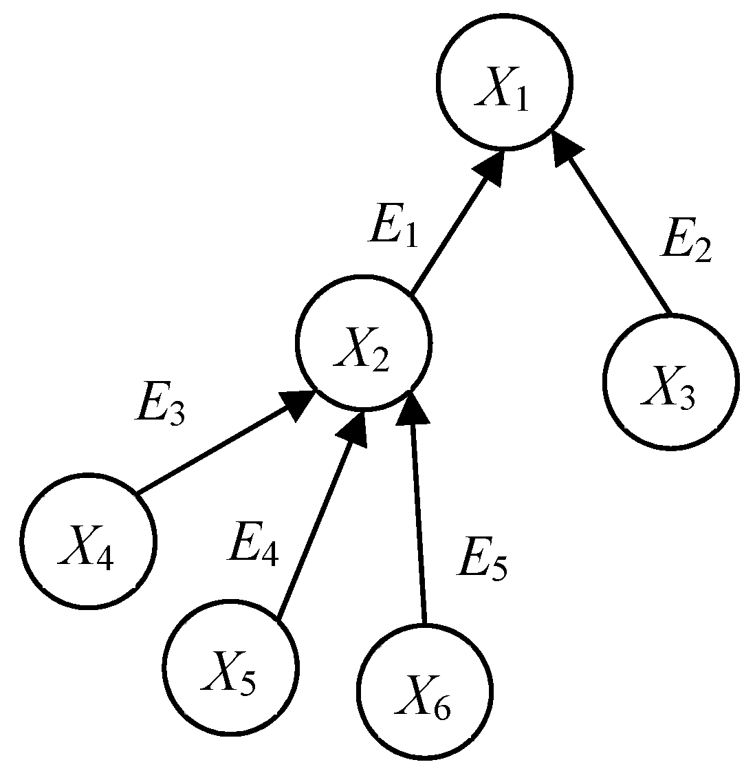
2.1.2. Establishment of Bayesian Network
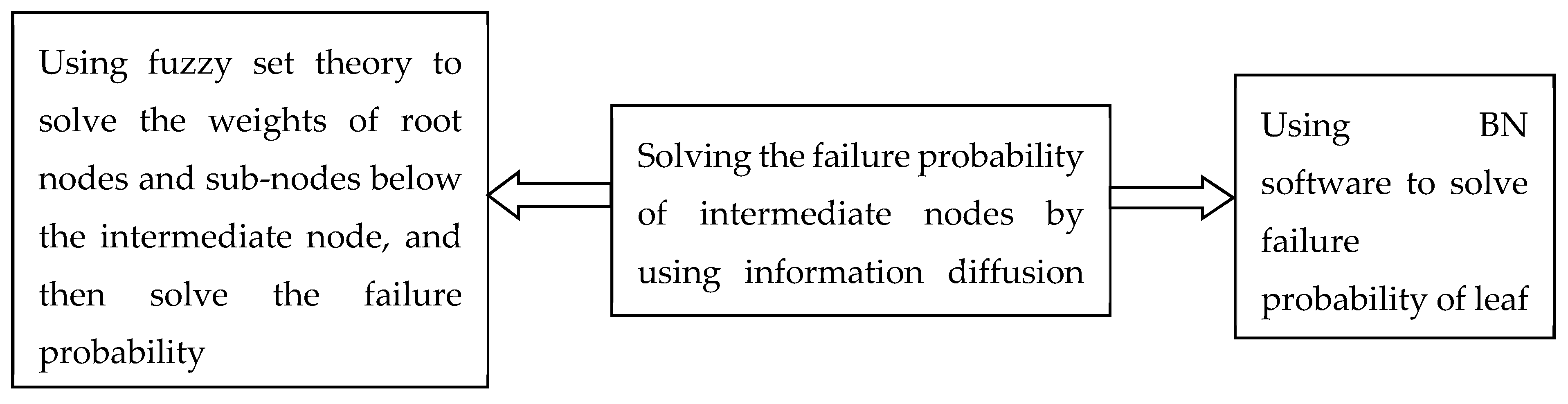
2.2. The Idea of Calculating Failure Probability
2.2.1. The Failure Probability of Intermediate Nodes
2.2.2. Fuzzy set theory
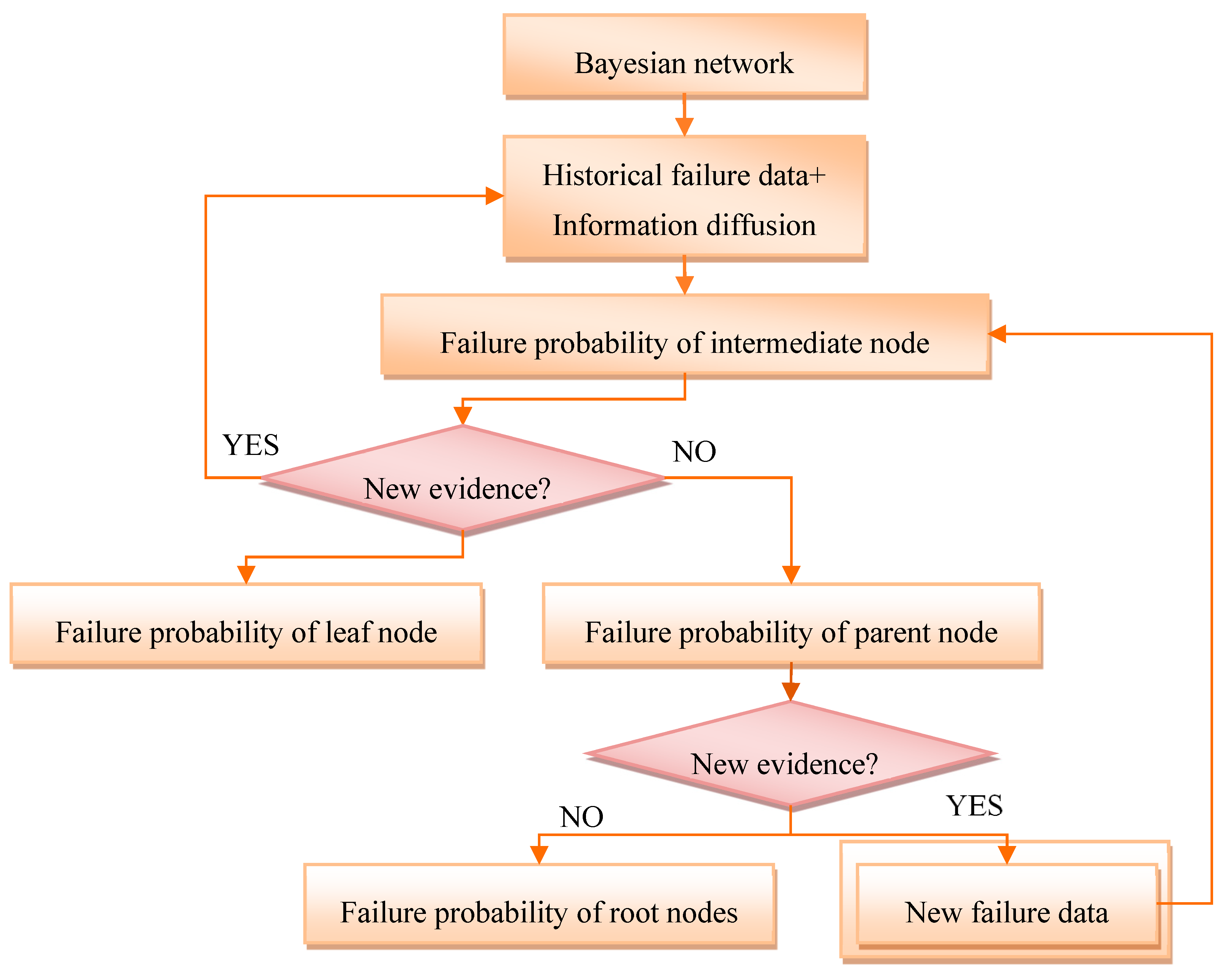
2.2.3. The updating of nodes failure probability in Bayesian Network
2.3. Assessment of Leakage Consequence Rating
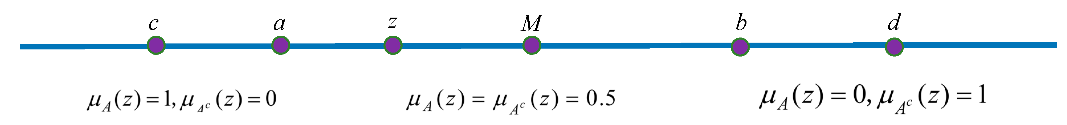
2.3.1. Variable Fuzzy Set Principle
2.3.2. Relative Difference Function Model
2.3.3. Comprehensive relative membership
2.3.4. Level eigenvalues and comprehensive evaluation
3. Case study
3.1. Establishment of BT Model
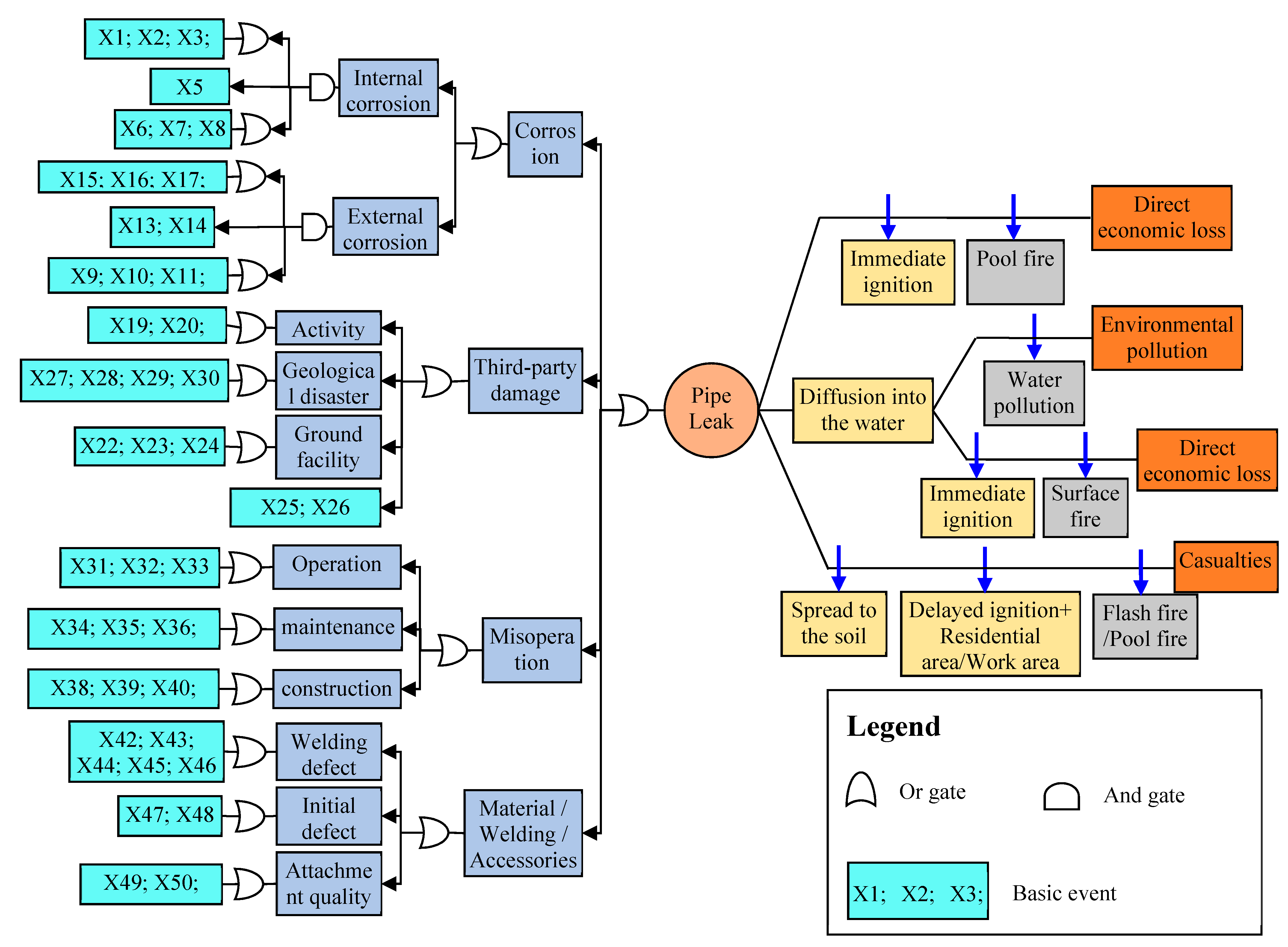
3.1.1. Risk Identification
- Third-party damageThe heavy oil gathering pipelines in the A oilfield are staggered vertically and horizontally, and there are more pipelines for parallel or crossing roads. Ground protection devices or protective measures are not in place. Here, the marking piles of pipelines are fewer in number and seriously damaged, where only the text can be distinguished. Moreover, it is generally considered that the linear direction between the wellhead and the metering station is the pipeline direction, which often results in serious construction damage. At last, due to the special geographical environment of the A oilfield, which is sparsely populated, locomotives often ignore the road and randomly shuttle, usually causing pipeline stress or fatigue damage.
- CorrosionCorrosion mainly includes internal corrosion and external corrosion. The medium transported by heavy oil gathering pipelines is generally a multi-phase flow with oil, gas, water, hydrocarbon and solid coexistence. The transport medium has a high degree of mineralization and can easily generate ions. There are also corrosive media such as dissolved oxygen, carbon dioxide, sulfides, and a large number of sulfate-reducing bacteria, along with mud sand, resulting in fouling, corrosion, and the abrasion of pipelines. On-site investigation of the corrosion causes of heavy oil gathering and transportation pipelines in the A oilfield mainly includes the following aspects: Some working areas have reservoirs, resulting in a high groundwater level, and water content in produced oil is ~85–92%, where some samples have high soil salinity. The transport medium contains more impurities, such as saprophytic bacteria, iron bacteria and sulfate reducing bacteria, etc. Some insulation layers are severely destroyed, and some are directly exposed to the outside, where the maintenance condition of which is not ideal. Moreover, the sulfur content in the produced oil is 0.34%, the acid value is 2.11 mg KOH/g, and the salt content is 15.93 mg of NaCl/L.
- MisoperationThere are many accessories and auxiliary facilities for heavy oil gathering pipelines, and the operators will make mistakes if they pay little attention to them. In the past accident records, accidental operation has caused pipelines to overpressurize and explode, to date resulting in the death of one staff member and many injuries. In addition, the frequency of regular safety training and job training is also one of the main sources of misoperation.
- Material/Welding/AccessoriesThe construction time of heavy oil gathering pipelines in the A oilfield is relatively long. Due to the welding technology level and the limited welding process at the time of pipeline construction, there is a large number of weld crack defects in the pipelines. With the long-term operation of the pipelines, the defects in initial small weld seams continue to expand and become larger, which brings about great hidden dangers to the safe operation of the pipeline. The quality of welding and maintenance will also directly affect the operating life of the pipelines. In the welding construction process, defects such as wear and dents often occur. If the defects are not discovered in time or are not fixed, they will become weak points of destruction during operation, especially in the later stages of service, where it is easy to induce damage. After on-site investigation, although the pipeline construction has been carried out by units with more than three years of construction experience, it has also been found that some construction misoperation still exists and that inspections are not in place. For example, anti-corrosion layers of different pipelines in the same operation area are very different. After running for many years, some are still intact, while some have already begun to fall off and even be destroyed. Leakage failure caused by weld defects occurs more frequently, which is inferred to be due to the quality of pipe welding construction. In addition, the maintenance situation is also uneven, and some pipeline accessories are exposed to the atmosphere and obviously fall off, but nobody cares.
3.1.2. Establishment of BT Model
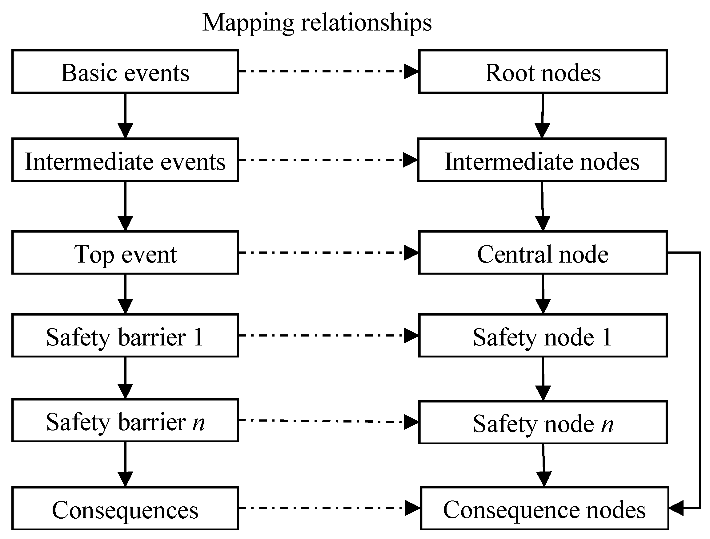
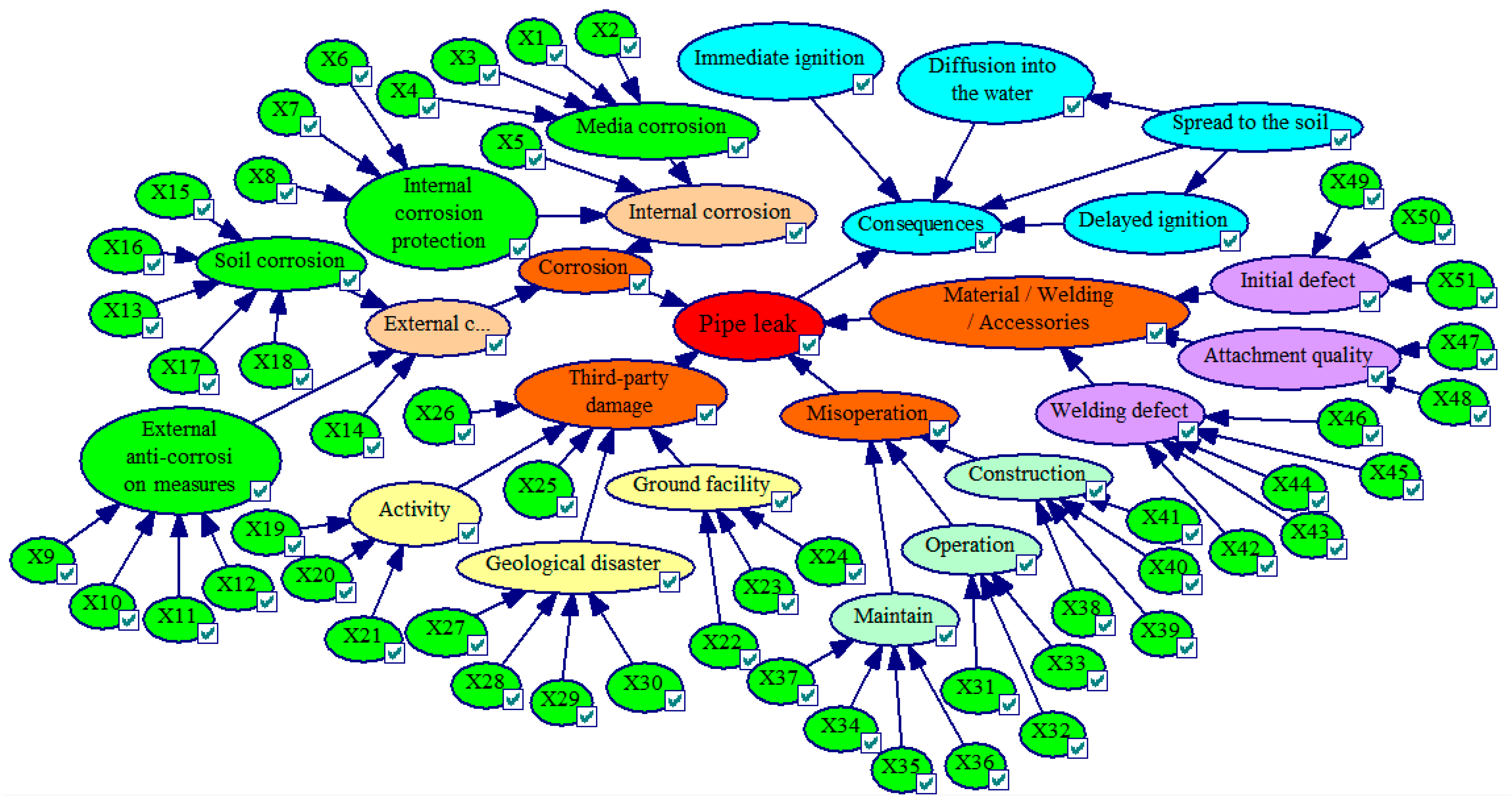
3.1.3. Conversion of BT model and BN
3.2. Failure Probability Calculation of Intermediate Nodes
3.3. Solution of the Leaf Node and Root Nodes’ Probability
3.4. Analysis of Failure Consequences of Heavy Oil Gathering Pipeline
3.4.1. Standard Interval of the Indicator Level
3.4.2. Determination of Comprehensive Membership
4. Conclusions
Author Contributions
Funding
Acknowledgments
Conflicts of Interest
References
- He, G.; Li, Y.; Lin, M.; Liao, K.; Liang, Y. Optimization of Gathering and Transmission Pipe Network Layout in Gas Field and Pipeline Route in 3D Terrain. J. Pipeline Syst. Eng. Pract. 2019, 10, 1190–1204. [Google Scholar] [CrossRef]
- Leung, T.; Hartloper, C.; Smith, J.; Botros, K.K.; Golshan, H.; Glenb, T. Application of EVM to determine pipe internal surface conditions in complex natural gas lateral networks. J. Nat. Gas Sci. Eng. 2015, 24, 217–227. [Google Scholar] [CrossRef]
- Zhang, P.; Qin, G.; Wang, Y. Risk assessment system for oil and gas pipelines laid in one ditch based on quantitative risk analysis. Energies 2019, 12, 981. [Google Scholar] [CrossRef] [Green Version]
- Muhlbauer, W.K. Pipeline Risk Management Manual, 3rd ed.; Gulf Publishing Companies: Houston, TX, USA, 2004; ISBN 978-0-7506-7579-6. [Google Scholar]
- Bertuccio, I.; Moraleda, M.V.B. Risk assessment of corrosion in oil and gas pipelines using fuzzy logic. Corros. Eng. Sci. Technol. 2012, 47, 553–558. [Google Scholar] [CrossRef]
- Arvind, K.R.M.; Chandima, R. Generic approach for risk assessment of offshore piping subjected to vibration induced fatigue. Corros. Eng. Sci. Technol. 2018, 4, 9017–9025. [Google Scholar]
- Abbas, R.; Banafsheh, Z.; Massoud, T. Integrated risk assessment of urban water supply systems from source to tap. Stoch. Environ. Res. Risk Assess. 2013, 27, 923–944. [Google Scholar]
- Cheliyan, A.S.; Bhattacharyya, S.K. Fuzzy fault tree analysis of oil and gas leakage in subsea production systems. J. Ocean. Eng. Sci. 2018, 3, 38–48. [Google Scholar] [CrossRef]
- Qi, J.; Hu, X.; Gao, X. Quantitative risk analysis of subsea pipeline and riser: An experts’ assessment approach using fuzzy fault tree. Int. J. Reliab. Saf. 2014, 8, 33–50. [Google Scholar] [CrossRef]
- Anjuman, S.; Rehan, S.; Solomon, T. Risk analysis for oil & gas pipelines: A sustainability assessment approach using fuzzy based bow-tie analysis. J. Loss Prev. Proc. Ind. 2012, 25, 505–523. [Google Scholar]
- Muniz, M.; Vinicios, P.; Lima, G.; Brito, A.; Caiado, R.G.G.; Quelhas, O.L.G. Bow tie to improve risk management of natural gas pipelines. Process Saf. Prog. 2018, 37, 169–175. [Google Scholar] [CrossRef]
- Dawotola, A.W.; Vrijling, J.K. Decision analysis framework for risk management of crude oil pipeline system advances in decision sciences. Adv. Decis. Sci. 2011, 2011, 456824. [Google Scholar]
- Bilal, Z.; Mohammed, K.; Brahim, H. Bayesian network and bow tie to analyze the risk of fire and explosion of pipelines. Process Saf. Prog. 2017, 36, 202–212. [Google Scholar] [CrossRef]
- He, R.; Li, X.; Chen, G. A quantitative risk analysis model considering uncertain information. Process Saf. Environ. Protect. 2018, 18, 361–370. [Google Scholar] [CrossRef]
- Alexander, G.U.; Atsushi, A. Pipeline risk assessment using artificial intelligence: A case from the colombian oil network. Process Saf. Prog. 2018, 37, 110–116. [Google Scholar]
- Shan, K.; Shuai, J.; Xu, K.; Zheng, W. Failure probability assessment of gas transmission pipelines based on historical failure-related data and modification factors. J. Nat. Gas Sci. Eng. 2018, 52, 356–366. [Google Scholar] [CrossRef]
- Li, X.; Chen, G.; Zhu, H.; Zhang, R. Quantitative risk assessment of submarine pipeline instability. J. Loss Prev. Proc. Ind. 2017, 45, 108–115. [Google Scholar] [CrossRef]
- Roberto, B. A statistical analysis of causes and consequences of the release of hazardous materials from pipelines. The influence of layout. J. Loss Prev. Process Ind. 2018, 56, 458–466. [Google Scholar]
- Ma, H.; Yuan, L.; Zhong, M.; Li, X.; Xie, Q.; Xie, X. Study on ground vibration mode of physical explosion of high pressure natural gas pipeline. Acoust. Phys. 2019, 65, 583–592. [Google Scholar]
- Zardasti, L.; Yahaya, N.; Valipour, A.; Rashid, A.S.A.; Noor, N.M. Review on the identification of reputation loss indicators in an onshore pipeline explosion event. J. Loss Prev. Process Ind. 2017, 48, 71–86. [Google Scholar] [CrossRef]
- Jang, C.B.; Choi, S.W.; Baek, J.B. CFD modeling and fire damage analysis of jet fire on hydrogen pipeline in a pipe rack structure. Int. J. Hydrog. Energy 2015, 40, 15760–15772. [Google Scholar] [CrossRef] [Green Version]
- Lyu, S.; Zhang, Y.; Wang, W.; Ma, S.; Huang, Y. Simulation Study on Influence of Natural Gas Pipeline Pressure on Jet Fire. IOP Conf. Ser. Earth Environ. Sci. 2019, 242, 1307–1315. [Google Scholar] [CrossRef]
- Lotoesmith, B.J. Large scale experiments to study fires following the rupture of high pressure pipelines conveying natural gas and natural gas/hydrogen mixtures. Process Saf. Environ. Protect. 2013, 91, 101–111. [Google Scholar] [CrossRef]
- Han, Z.Y.; Weng, W.G. Comparison study on qualitative and quantitative risk assessment methods for urban natural gas pipeline network. J. Hazard. Mater. 2011, 189, 509–518. [Google Scholar] [CrossRef] [PubMed]
- Kabir, S.; Papadopoulos, Y. Applications of Bayesian networks and Petri nets in safety, reliability, and risk assessments: A review. Saf. Sci. 2019, 115, 154–175. [Google Scholar] [CrossRef]
- Abimbola, M.; Khan, F.; Khakzad, N.; Butt, S. Safety and risk analysis of managed pressure drilling operation using Bayesian network. Saf. Sci. 2015, 76, 133–144. [Google Scholar] [CrossRef]
- Cattaneo, M.E.G.V. The likelihood interpretation as the foundation of fuzzy set theory. Int. J. Approx. Reason. 2017, 90, 333–340. [Google Scholar] [CrossRef]
- Diker, M. Textures and fuzzy unit operations in rough set theory: An approach to fuzzy rough set models. Fuzzy Sets Syst. 2018, 336, 27–53. [Google Scholar] [CrossRef]
- Zhang, Q.; Lv, H.; Yang, Y. Effect evaluation of high-speed railway skylight construction based on triangular fuzzy number. J. Southwest Jiaotong Univ. 2018, 53, 798–805. [Google Scholar]
- Li, Y. Environmental risk assessment of natural gas gathering and transportation pipeline based on fuzzy comprehensive evaluation. Channel Sci. 2014, 6, 47–51. [Google Scholar]
- Qin, C. Safety risk analysis of natural gas gathering and transportation pipeline based on PHA. J. Inner Mong. Petrochem. Ind. 2015, 41, 67–68. [Google Scholar]
- Zeng, X. Research and Application of risk Assessment Technology for gathering and Transportation Pipeline. J. Chem. Manag. 2018, 21, 153. [Google Scholar]
- Mandal, P.; Ranadive, A.S. On the structure of fuzzy variable precision rough sets based on generalized residuted lattices. J. Intell. Fuzzy Syst. 2017, 32, 483–497. [Google Scholar] [CrossRef]
- Jia, J.; Wang, X.; Naima, A.M.H.; Zhao, W.; Liu, Y. Flood-Risk Zoning Based on Analytic Hierarchy Process and Fuzzy Variable Set Theory. Nat. Hazards Rev. 2019, 20, 6988–6996. [Google Scholar] [CrossRef]
- Wang, W.C.; Xu, D.M.; Chau, K.W.; Lei, G.J. Assessment of River Water Quality Based on Theory of Variable Fuzzy Sets and Fuzzy Binary Comparison Method. Water Resour. Manag. 2014, 28, 4183–4200. [Google Scholar] [CrossRef]
- Aggarwal, M. Probabilistic variable precision fuzzy rough sets. IEEE Trans. Fuzzy Syst. 2016, 24, 29–39. [Google Scholar] [CrossRef]
- Chen, S.; Guo, Y. Variable fuzzy sets and its application in comprehensive risk evaluation for flood—Control engineering system. Fuzzy Optim. Decis. Mak. 2006, 5, 153–162. [Google Scholar]
- Chen, S.; Xue, Z.; Li, M. Variable Sets principle and method for flood classification. Sci. China-Technol. Sci. 2013, 56, 2343–2348. [Google Scholar] [CrossRef]
- Li, P. Research on Safety Evaluation of Existing Buildings Based on the Theory Variable Fuzzy Sets. Ph.D. Thesis, Xi’an University of Architecture and Technology, Xi’an, China, 2016. [Google Scholar]
- Zhang, H.B. Research on Quantitative Risk Evaluation Technology of Long-Term Natural Gas Pipelines Based on Failure Database. Ph.D. Thesis, China University of Geosciences, Beijing, China, 2013. [Google Scholar]

| Nodes | X1 | X5 | ||
|---|---|---|---|---|
| State | Y | N | Y | N |
| Probability | 0.3 | 0.7 | 0.8 | 0.2 |
| (X2, X3) | |||||
|---|---|---|---|---|---|
| X2 = Y | X2 = N | ||||
| X3 = Y | X3 = N | X3 = Y | X3 = N | ||
| X1 | P1 | P2 | P3 | P4 | |
| 1 − P1 | 1 − P2 | 1 − P3 | 1 − P4 | ||
| P | P1 | P2 | P3 |
|---|---|---|---|
| P1 | (1,1,1) | (1,1.5,2) | (1.5,2,2.5) |
| (0.5,1,1.5) | (1.5,2,2.5) | ||
| (1.5,2,2.5) | (1.5,2,2.5) | ||
| P2 | (1/2,1/1.5,1/0.5) | (1,1,1) | (1.5,2,2.5) |
| (1/0.5,1,1/0.5) | (1,1.5,2) | ||
| (1/2.5,1/2,1/1.5) | (0.5,1,1.5) | ||
| P3 | (1/2.5,1/2,1/1.5) | (1/2.5,1/2,1/1.5) | (1,1,1) |
| (1/2.5,1/2,1/1.5) | (1/2,1/1.5,1) | ||
| (1/2.5,1/2,1/1.5) | (1/1.5,1,1/0.5) |
| [1,1.5) | [1.5,2) | [2,2.5) | [2.5,3) | [3,3.5) | [3.5,4] | |
| Rank | Level 1 | Level 2- | Level 2+ | Level 3- | Level 3+ | level 4 |
| No. | Description | No. | Description |
|---|---|---|---|
| X1 | H2S content | X27 | earthquake |
| X2 | CO2 content | X28 | landslide |
| X3 | the free water content | X29 | debris flow |
| X4 | the chloride content | X30 | ground subsidence |
| X5 | the pipeline operation period | X31 | staff training |
| X6 | the internal coating | X32 | the operating procedure |
| X7 | the corrosion inhibitor | X33 | the SCADA communication system |
| X8 | pipe pigging | X34 | the maintenance plan |
| X9 | the external coating material | X35 | the maintenance procedure |
| X10 | external coating defects | X36 | the maintenance method |
| X11 | insulation stripping | X37 | the maintenance work check |
| X12 | cathodic protection | X38 | a coated mouth |
| X13 | stray current | X39 | backfill quality |
| X14 | the time of using an external anti-corrosion layer | X40 | construction inspection |
| X15 | the soil PH | X41 | poor geological conditions |
| X16 | salt content | X42 | welding inspection |
| X17 | soil porosity | X43 | the welding method |
| X18 | soil resistivity | X44 | porosity |
| X19 | construction activity | X45 | slag |
| X20 | traffic activity | X46 | not welded |
| X21 | terrorist activities | X47 | the poor quality of accessories |
| X22 | the line sign | X48 | installation is not standardized |
| X23 | stacking pressure | X49 | a crack |
| X24 | ground device protection | X50 | a scratch |
| X25 | the covering soil thickness | X51 | a depression defect |
| X26 | pipe diameter |
| Years | Intermediate Node (Reasons) | |||
|---|---|---|---|---|
| Corrosion | Third-Party Damage | Misoperation | Material/Welding/Pipe Accessories | |
| 2011 | 355 | 3 | 2 | 214 |
| 2012 | 312 | 6 | 6 | 128 |
| 2013 | 532 | 3 | 10 | 63 |
| 2014 | 520 | 5 | 8 | 212 |
| 2015 | 423 | 2 | 5 | 115 |
| 2016 | 256 | 4 | 3 | 84 |
| Years | Average Failure Probability | |||
|---|---|---|---|---|
| Corrosion | Third-Party Damage | Misoperation | Material/Welding/Pipe Accessories | |
| 2011 | 0.0374 | 0.000316 | 0.000211 | 0.0225 |
| 2012 | 0.0328 | 0.000632 | 0.000632 | 0.0135 |
| 2013 | 0.0560 | 0.000316 | 0.0011 | 0.0066 |
| 2014 | 0.0547 | 0.000526 | 0.000844 | 0.0223 |
| 2015 | 0.0445 | 0.000211 | 0.000526 | 0.0121 |
| 2016 | 0.0269 | 0.000422 | 0.000316 | 0.0088 |
| No. | Description | P0 | Sequence | No. | Description | P0 | Sequence |
|---|---|---|---|---|---|---|---|
| X1 | CO2 content | 1.46 × 10⁻³ | 3 | X27 | Earthquake | 1.56 × 10⁻⁵ | 48 |
| X2 | H2S content | 1.51 × 10⁻³ | 4 | X28 | Landslide | 4.18 × 10⁻⁶ | 51 |
| X3 | Free water content | 1.08 × 10⁻³ | 6 | X29 | Debris flow | 4.60 × 10⁻⁵ | 45 |
| X4 | Chloride content | 2.56 × 10⁻⁴ | 22 | X30 | Ground subsidence | 1.51 × 10⁻⁵ | 49 |
| X5 | Pipeline operation period | 1.96 × 10⁻³ | 1 | X31 | Staff training | 1.74 × 10⁻⁴ | 30 |
| X6 | Internal coating | 1.10 × 10⁻³ | 7 | X32 | Operating procedure | 7.43 × 10⁻⁵ | 40 |
| X7 | Corrosion inhibitor | 1.68 × 10⁻³ | 2 | X33 | SCADA communication system | 3.68 × 10⁻⁵ | 47 |
| X8 | Pipe pigging | 4.53 × 10⁻⁴ | 15 | X34 | Maintenance plan | 8.26 × 10⁻⁵ | 39 |
| X9 | External coating material | 1.23 × 10⁻⁴ | 33 | X35 | Maintenance procedure | 1.07 × 10⁻⁴ | 37 |
| X10 | External coating defect | 3.27 × 10⁻⁴ | 20 | X36 | Maintenance method | 1.85 × 10⁻⁴ | 29 |
| X11 | Insulation stripping | 2.18 × 10⁻⁴ | 26 | X37 | Maintenance work check | 1.12 × 10⁻⁴ | 35 |
| X12 | Cathodic protection | 4.23 × 10⁻⁴ | 18 | X38 | Coated mouth | 2.25 × 10⁻⁴ | 24 |
| X13 | Stray current | 1.89 × 10⁻⁴ | 28 | X39 | Backfill quality | 9.56 × 10⁻⁵ | 38 |
| X14 | Time of using external anti-corrosion layer | 1.01 × 10⁻³ | 8 | X40 | Construction inspection | 6.24 × 10⁻⁵ | 42 |
| X15 | Soil PH | 5.11 × 10⁻⁴ | 13 | X41 | Poor geological conditions | 3.74 × 10⁻⁵ | 46 |
| X16 | Salt content | 5.11 × 10⁻⁴ | 13 | X42 | Welding inspection | 7.29 × 10⁻⁴ | 10 |
| X17 | Soil porosity | 1.47 × 10⁻⁴ | 32 | X43 | Welding method | 6.44 × 10⁻⁵ | 41 |
| X18 | Soil resistivity | 2.93 × 10⁻⁴ | 21 | X44 | Porosity | 1.19 × 10⁻⁴ | 34 |
| X19 | Construction activity | 8.28 × 10⁻⁶ | 9 | X45 | Slag | 2.37 × 10⁻⁴ | 23 |
| X20 | Traffic activity | 2.22 × 10⁻⁵ | 25 | X46 | Not welded | 4.42 × 10⁻⁴ | 16 |
| X21 | Terrorist activities | 1.27 × 10⁻⁶ | 50 | X47 | Poor quality of accessories | 6.35 × 10⁻⁴ | 11 |
| X22 | Line sign | 5.77 × 10⁻⁵ | 43 | X48 | Installation is not standardized | 1.48 × 10⁻³ | 5 |
| X23 | Stacking pressure | 5.10 × 10⁻⁵ | 44 | X49 | Crack | 1.92 × 10⁻⁴ | 27 |
| X24 | Ground device protection | 1.11 × 10⁻⁴ | 36 | X50 | Scratch | 4.29 × 10⁻⁴ | 17 |
| X25 | Staff training | 1.67 × 10⁻⁴ | 31 | X51 | Depression defect | 3.33 × 10⁻⁴ | 19 |
| X26 | Pipe diameter | 6.02 × 10⁻⁵ | 12 |
| Consequence Level | General Accident (Level 1) | Large Accident (Level 2) | Major Accident (Level 3) | Special Major Accident (Level 4) |
|---|---|---|---|---|
| Personal injury/person | ~0–0.5 | ~0.5–1 | ~1–3 | ~3–10 |
| Direct economic loss/100 million ¥ | ~0–0.1 | ~0.1–0.5 | ~0.5–1 | ~1–2 |
| Environmental damage recovery/million ¥ | ~0–10 | ~10–50 | 50–100 | ~100–500 |
| Social impact coefficient | ~0–0.2 | ~0.2–0.5 | ~0.5–0.7 | ~0.7–1 |
| Year | Type of Consequence | |||
|---|---|---|---|---|
| Personal Injury/Person | Direct Economic Loss/100 Million ¥ | Environmental Damage Recovery/Million ¥ | Social Impact Coefficient | |
| 2011 | 0.2 | 0.30 | 164 | 0.57 |
| 2012 | 0.6 | 0.42 | 149 | 0.45 |
| 2013 | 0.8 | 0.32 | 194 | 0.61 |
| 2014 | 0.7 | 0.24 | 214 | 0.60 |
| 2015 | 0.4 | 0.34 | 161 | 0.76 |
| 2016 | 0.3 | 0.20 | 114 | 0.34 |
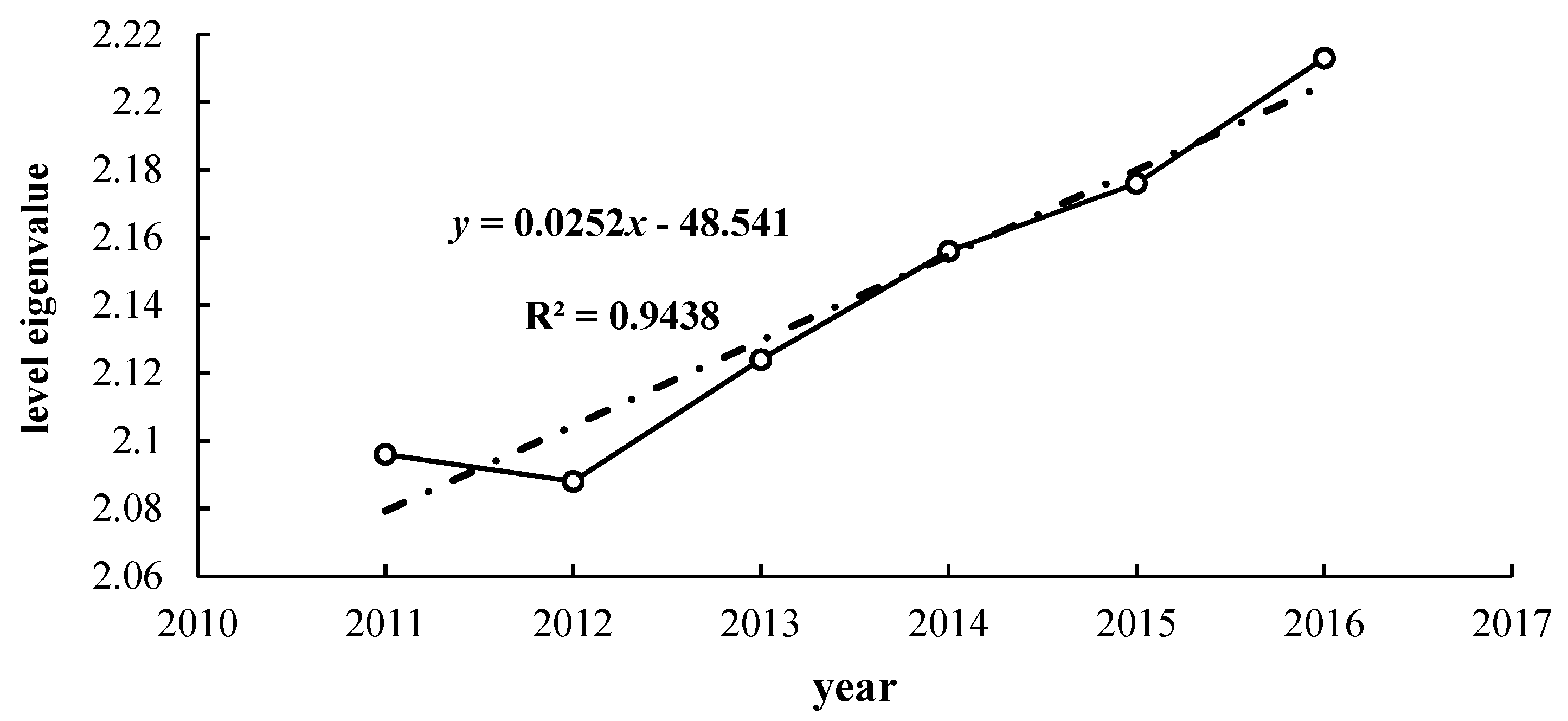
| Year | Normalized Membership under Parameter Combination | Mean Level Eigenvalues | Grade | |||
|---|---|---|---|---|---|---|
| α = 1, p = 1 | α = 1, p = 2 | α = 2, p = 1 | α = 2, p = 2 | |||
| 2011 | 2.768 | 1.780 | 1.811 | 2.022 | 2.096 | Level 2- |
| 2012 | 1.952 | 2.063 | 2.488 | 2.057 | 2.088 | Level 2- |
| 2013 | 2.097 | 2.107 | 2.104 | 2.189 | 2.124 | Level 2- |
| 2014 | 2.163 | 2.172 | 2.105 | 2.183 | 2.156 | Level 2- |
| 2015 | 2.353 | 2.109 | 2.108 | 2.134 | 2.176 | Level 2- |
| 2016 | 2.384 | 2.172 | 2.109 | 2.185 | 2.213 | Level 2- |
© 2020 by the authors. Licensee MDPI, Basel, Switzerland. This article is an open access article distributed under the terms and conditions of the Creative Commons Attribution (CC BY) license (http://creativecommons.org/licenses/by/4.0/).
Share and Cite
Zhang, P.; Chen, X.; Fan, C. Research on a Safety Assessment Method for Leakage in a Heavy Oil Gathering Pipeline. Energies 2020, 13, 1340. https://doi.org/10.3390/en13061340
Zhang P, Chen X, Fan C. Research on a Safety Assessment Method for Leakage in a Heavy Oil Gathering Pipeline. Energies. 2020; 13(6):1340. https://doi.org/10.3390/en13061340
Chicago/Turabian StyleZhang, Peng, Xiangsu Chen, and Chaohai Fan. 2020. "Research on a Safety Assessment Method for Leakage in a Heavy Oil Gathering Pipeline" Energies 13, no. 6: 1340. https://doi.org/10.3390/en13061340