Abstract
Sprinkler activation is one of the key events defining the course of a compartment fire. The time when activation occurs is commonly used in the determination of the design fire scenario, which is the cornerstone of the design of building fire safety features. A well-known model of sprinkler activation (response time index (RTI) model) was introduced into the numerical scheme of the ANSYS Fluent computational fluid dynamics (CFD) package. The novel way in which the model is used is the calculation of the time for sprinkler activation within each discrete cell of the domain. The proposed novel approach was used in a case-study to assess the effects of comfort mode natural ventilation on a sprinkler’s activation pattern. It was found that hinged vents in the comfort mode had a significant effect on sprinkler activation, both in terms of delaying it as well as limiting the total number of cells in which the sprinkler would have activated. In some scenarios with a hinged vent, no activation was observed in the central point of the vent, possibly indicating problems with the autonomous triggering of the fire mode of such a device. It was also found that the RTI and C (related to the conductive transport of sprinkler fitting) parameter values had a moderate influence on sprinkler activation time—only for high-temperature sprinklers (≥ 141 °C). This study shows the applicability of the 3D activation time mapping for research focused on the fire safety of sprinkler-protected compartments and for the performance-based approach to sprinkler system design. Even though the RTI model is the industry standard for the determination of sprinkler response, the model implementation in ANSYS Fluent was not validated. This means that sources of uncertainty, mainly connected with the determination of flow velocity and temperature are not known, and the model should be used with caution. An in-depth validation is planned for subsequent studies.
1. Introduction
Sprinkler protection is paramount to the fire safety of buildings. Sprinkler systems, with a notable mention of Early Suppression Fast Response sprinklers used in the highest risk industrial applications, must deliver large amounts of water as quickly as possible. However, the complex architecture of buildings and the use of ventilation systems could cause air flows that may adversely affect sprinkler activation time. In general, sprinklers are placed uniformly in a dense network covering an entire compartment. If a sprinkler grid interacts with vents, design standards such as the NFPA 13 [1] or the VdS 2815 guidance document [2] forbid the use of automatically-activated natural vents. In contrast, some law systems, such as the Polish building code, require the use of such a smoke ventilation system, leaving the responsibility of minimizing the adverse effects of ventilation on the system designer. Furthermore, many industrial and warehouse buildings use natural ventilation in day-to-day comfort mode, and such installations are so far not considered as a severe threat to the sprinkler operation.
Besides the adverse effect of ventilation, other elements (e.g., obstacles, beams, and openings) that influence the flow of heat and mass in the upper smoke layer may also adversely affect sprinkler operation. Such effects are not entirely understood, presumably due to the high cost of building-scale of fire experiments on sprinkler and vent operation and the lack of simple models that would allow for the investigation of sprinkler activation time over an area or volume.
The goal of this paper is to introduce a novel approach—the 3D mapping of sprinkler activation time. The proposed solution is an introduction of a well-known response time index (RTI) model [3] into the numerical scheme of the vastly validated general-purpose computational fluid dynamics (CFD) code of ANSYS Fluent. The introduced model allows for a simultaneous assessment of the potential activation of sprinklers over a volume for a supplied array of user-defined variables defining sprinklers and the evolution of fires. In this paper, the implementation of the new tool is presented, and a case-study is carried out where the effects of comfort mode day-to-day natural ventilation on sprinkler activation time in a high-rack storage facility is assessed with the new approach.
2. The RTI Model
In 1976, Heskestad et al. introduced the RTI as a measure of the responsiveness of a sprinkler link. They assumed that the link acted as a thermally thin body that is heated by the hot gases coming from the fire plume [4]. Upon reaching the activation time, the link undergoes transition (bulb breaks due to vapor pressure or bimetal link bends due to thermal stress), which triggers the release of water in sprinklers. The same mechanism rules the activation of the release mechanism in vents. Neglecting radiation from the flame and conduction losses to the sprinkler head, they proposed the following response behavior:
where u is the velocity of the hot gases; Tg and Te are consequently the gas phase and the thermal element (bulb) temperatures, respectively; and the RTI is a constant that, in principle, depends on the thermal properties of the sprinkler link only. For certain flow conditions (constant flow velocity and gas temperature), Equation (1) can be analytically integrated, and the RTI can be solved for. The plunge test that Heskestad et al. also proposed in their report provided the conditions for an analytic solution so that sprinkler links could be easily classified and compared. This method led to the development of new sprinkler technologies such as Early Suppression Fast Response (ESFR) and quick response residential fire sprinklers. This ground-breaking innovation had a significant impact on the building, fire, and electrical safety fields, and it was awarded prestigious NFPA 2019 Philip J. DiNenno Prize [5].
It soon became apparent that for low gas velocities that are typically found in slowly growing fires, the RTI was not constant, as conductive losses to sprinkler fittings could no longer be neglected [6]. Heskestad and Bill then proposed a modified response behavior that gave origin to a two-parameter model [3]:
where C is a parameter related to conductive transport to the sprinkler fitting. While the model showed an improved agreement with the experimental results, the dependence on a second parameter made the classification somewhat more complicated. Alternative but similar approaches were presented by Thorne et al. [7] and Melinek [8]. Heskestad and Bill’s model was experimentally assessed by Frank et al., who inserted thermocouples into modified sprinkler bulbs to measure the actual bulb temperature when exposed to hot gases as a function of time [9]. They found that the modelled bulb temperature evolution matched the experimental curve closely in the case of the plunge tests, but they detected considerable differences when using ceiling jet temperature and velocity data from compartment fire experiments, especially for fast-growing fires.
A more sophisticated model for sprinkler link temperature was presented by You et al. [10]. They proposed to include radial dependence in the temperature inside the link and provided analytic and numerical solutions for the resulting equations.
The simplicity of Equations (1) and (2) makes it reasonably straightforward to implement them in combination with commonly used fire models. Since gas temperature and velocity in those cases are generally not constant, it is necessary to solve the equations numerically (typically using some Runge–Kutta scheme). An early attempt was presented by Evans and Stroup [11,12], who solved Equation (1) with gas temperatures using Alpert’s correlations [13]. Davis and Cooper included the heat contribution of the upper layer that accumulates in confined ceilings [14], implementing a zone model complemented by a ceiling jet algorithm, that provided more realistic temperatures for the sprinkler link model. The zone model BRANZFIRE implements both Davis’ jet model and Alpert’s correlations for sprinkler activation, and the relative performance was later assessed by Wade et al. [15] by comparing simulated response time to experimental values. They confirmed the expected superior performance of Davis’ algorithm over Alpert’s correlations. Joglar et al. recognized the fact that several of the parameters that need to be input into the model are often poorly defined, and they consequently proposed a probabilistic approach to the sprinkler activation problem (although the underlying model is still a deterministic zone model with a ceiling jet algorithm) [16].
The first attempt of predicting sprinkler activation times using a CFD fire model was made by Tuovinen [17], who used the CFD code JASMINE to calculate link temperatures based on the original RTI model (without considering conductive losses to the sprinkler fittings). The author concluded that JASMINE overestimated ceiling jet temperatures but underestimated flow velocities. While no comparison to experimental sprinkler activation times was made, a possible influence of ventilation was detected due to a simulated delay in activation near openings.
The fire dynamics simulator (FDS) is the most widely used CFD-based fire model. A numerical solution to Equation (2) has been included in FDS from the very beginning. Early validation efforts of the sprinkler activation times were presented by McGrattan et al. [18] and Olenick et al. [19]. Both assessed the prediction of sprinkler activation times when compared to experimental values in high rack storage fires, and they reported good agreement. The validation of the sprinkler activation model was revisited by Bittern [20], who compared activation time predictions from FDS version 3 to experimental values reported in [15]. The main conclusion from that study was that the value of the C parameter (Equation (2)) and the position of the fire affect the performance of the model. In the case of the fire being located in the center of the room, predictions agreed well with the experiments, while results were less favorable if the fire was located in the corner of the compartment.
Hopkin and Spearpoint [21] provided a comparative study on sprinkler activation times, using different versions of the same model (FDS versions 3 and 6) with varying modelling assumptions. Three new sprinkler activation simulations were presented and compared to Bittern’s [20] original simulation; the first corresponded to Bittern’s simulations (same input parameters) but used the (then) latest version of FDS (version 6.6.0). The improved physics implemented in FDS version 6 produced a marginal improvement in terms of difference to experimental values. A second simulation run by Hopkin and Spearpoint considered a fire area closer to the one reported in the experiments (0.2 m2 instead of 0.04 m2, as used by Bittern). The last simulation provided was run with a smaller C-factor (0.4 m1/2s−1/2 instead of 0.65 m1/2s−1/2) and a finer grid (0.05 m edge size instead of 0.1 m). Interestingly, the activation times of the last model improved considerably, while the ceiling jet temperature was over-predicted more than in the other two simulations when compared to the experimental measurements. This indicates that similarly to Touvinen’s reasoning, the flow velocity was underestimated, thus balancing out when estimating the sprinkler link temperature.
3. Creating a 3D Map of the Sprinkler Activation Time
The novel approach presented in this paper is related to the simultaneous spatial assessment of sprinkler activation time in every cell of the numerical domain. In previous approaches such as hand calculation methods that employed Alpert’s ceiling jet [13], the early computer model DETACT [22], zone models [23], and modern CFD tools [24], the RTI model has been used to determine whether activation conditions are met at a predefined point in space (sprinkler link). To generalize the results for common design fires and typical architecture, the same approach was used to calculate tables of sprinkler activation time, which became an essential part of the German standard VDI 6019 [25]. All of these methods enabled the answering of the question “When will this sprinkler activate?”, but they failed to provide information related to the activation of sprinklers in different locations. For such an analysis, arrays of sprinkler devices must be created. Considering the capabilities of previously mentioned models, this would have been a daunting and cumbersome task.
For a more elegant solution to this problem, the RTI model was implemented in a novel way within the well-known general-purpose CFD code ANSYS Fluent. The new approach simultaneously determines the sprinkler activation time in every finite cell of the considered control volume (computational domain) in every time step of the analysis. This was achieved by applying a dedicated user defined function (UDF), which tracks the temperature of a sprinkler bulb as if it was located in a given cell during fire evolution. The formula introduced by Heskestad and Bill (Equation (2)) including the C-parameter was used for this purpose. User defined memory (UDM) slots are used to store the three variables related to the problem: activation time, bulb temperature, and activation indicator.
Equation (2) describes the rate of change of sprinkler link temperature. This equation is independently solved for every cell of the model in each time-step, based on the gas temperature and airflow velocities within that cell. If the link temperature reaches the actuation threshold (TACT) in a given time step, the sprinkler is regarded as activated. In this time step, each cell in which the activation occurred is given a new value of activation time variable, which is equal to the current time in the simulation (at the moment of activation). The activation also causes the cell to be flagged as “activate” which prevents further calculations of the link temperature.
The user-defined variables required for the calculation include the actuation threshold temperature (TACT), the RTI value and the C-parameter that describes the conduction characteristics of the sprinkler head. The results are saved as three variables. The first variable contains the previous time step, the second is the previously calculated bulb temperature, and the last variable is the flag that marks whether a given sprinkler has been already activated. This allows for the determination of the current bulb temperature (according to Equation (2)), then the values of the first two variables are updated, and in the case of sprinkler activation, the third variable is set to a non-zero value. As a result, a 3D distribution of the activated sprinklers of different types is obtained; and in the case of a sprinkler activation, a time moment of this event is known.
User-defined variables may be supplied as lists of parameters. The sprinkler activation calculation UDF will solve for each combination separately using different UDM slots. The only hard limit is the 500 UDM slots available in the ANSYS Fluent solver.
Though Equation (2) was semi-empirically derived for static experiment conditions, it was here assumed that due to a short simulation time step it is allowable to apply it for a dynamic process. In such a way, the temperature change for a bulb is determined for every time step. An additional simplification concerns the term containing the C-parameter. This term describes heat losses due to conductivity, and its value depends on the temperature difference between a sprinkler and its mounting. Since the latter is in general unknown, the initial temperature was used here. Such an approach is commonly adopted because only the initial stage of a fire is considered (before sprinkler activation) when construction elements have not yet heated up.
The proposed implementation of the RTI model in the commercial code ANSYS Fluent was not validated. The validation of the model in numerical tools exists for simple model DETACT [22], zone models [15], and CFD code FDS [20,21]. Based on the similarities between these tools and ANSYS Fluent, we assumed that the uncertainty of sprinkler activation time with ANSYS Fluent would be similar. We consider this justified for this paper, as the study was focused on the idea of 3D mapping as a novel approach in investigation of the sprinkler activation patterns and on the ideas of how such approach may be used in research and engineering. However, for future research on interactions of smoke control and sprinklers, a more detailed model validation is necessary. Such research is already in progress and will be published in subsequent papers.
4. Case Study—Numerical Model
To demonstrate the capabilities of the 3D mapping of the sprinkler activation time, the effect of natural ventilation on the activation of sprinklers located above a high-storage rack in a warehouse was investigated. This was a typical case where a natural ventilation system is used in a comfort mode ventilation of the facility, meaning that the vents are partially open for a prolonged time. In this mode of operation, the vents typically open to an angle between 10° and 15°; while in fire mode operation, the standard opening angle is 140°–165°. The natural ventilation system in comfort mode may be operating during the beginning of the fire, potentially allowing hot gases to escape through the opening, presumably leading to a delay in sprinkler activation in the vent vicinity. A quantitative analysis of the vent effect on sprinklers with a traditional approach would require the creation of an array of potential sprinklers near the vent. In the activation time mapping approach, the time of activation of sprinklers in the proximity of the vent is simply drawn as an image for every combination of the input parameters, allowing for a more accessible visual assessment of its effects.
A CFD analysis was performed using the ANSYS Fluent software package, with an unsteady k-ε (realizable) turbulence model. This solver has been widely used in fire research analyses and is recognized by some of the smoke control standards [26]. Some validation examples for ANSYS Fluent were given in [27,28,29,30,31]. The principal assumptions for numerical calculations and the choice of physical sub-models are summarized in Table 1.

Table 1.
Summary of the user-defined solver settings in the computational fluid dynamics (CFD) analyses.
A 3D model of a warehouse (L: 60 m, W: 40 m, H: 8 m) facility was created. The storage height was chosen as 6 m. A view of the model and the fire source is shown in Figure 1. The facility was equipped with natural smoke control system dimensioned following NFPA 204 guidance [32]. Six vents, with dimensions of 1.80 × 1.50 m, were uniformly distributed on the warehouse roof. The opening angle for sanitary mode operation was chosen as 15°.
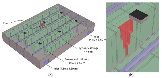
Figure 1.
(a) The numerical model of a high-storage facility, open natural ventilator (top left), and (b) the detailed view on the source of fire and closed ventilator.
Three different fires that differed in the growth coefficient and the maximum heat release rate (HRR) were assessed. The fires were introduced as a volumetric source of heat and mass (smoke). The maximum HRR per unit of volume of the source was set to 2 MW/m3. The HRR evolution in fire scenarios 1 and 2 followed Equation (3).
where is the HRR of the fire, t is time, and α is the fire growth coefficient, taking the value of 0.047 kW/s2 (so-called “fast”) for fire scenario 1 and 0.188 kW/s2 (so-called “ultrafast”) for fire scenario 2.
The fire scenario 3 followed Equation (4):
where the fire growth coefficient value, α, of 0.00408 kW/s3 was calculated for storage height of 6 m following New Zealand’s C/VM2 document [33]. The fire scenarios were not meant to represent a particular threat in a warehouse storage facility but rather a wide array of potential fires that may occur in such a compartment. Simulation time was limited to 600 s. The maximum HRR was arbitrarily capped at 4.23 MW for fire scenario 1 and at 9.00 MW for fire scenarios 2 and 3. In the case of fire scenarios 2 and 3, the maximum HRR of 9 MW was reached after 218 and 130, s respectively. The production of smoke was described through a soot yield coefficient, for which a conservative value of 0.1 g/g was chosen [34].
Wind effects were not considered in this simulation. It should be noted that the wind may have a significant effect on natural ventilation performance [35,36] and consequently on sprinkler activation pattern and activation time. The sprinkler activation mapping approach presented herein may be effectively used to assess such effects and will be the goal of subsequent research performed by the authors.
The case study included 3 values of RTI, 4 values of sprinkler activation temperature, and 3 values of conductivity parameter, which gave 36 possible combinations of these parameters (and 108 UDM slots), as shown in Table 2.
Table 2.
The matrix of scenarios and user-defined variables used in this examination.
The numerical model was discretized with an unstructured tetrahedral mesh (maximum element dimension δi = 0.4 m) in most of the domain and with a structured Cartesian mesh (maximum element dimension δx = 0.1 m) in the area above the fire and in the proximity of the vents. The meshes were connected with the use of a mesh growth function, with a 1.30 mesh growth factor. A sample view of the numerical mesh in the vicinity of the ventilator (the area where sprinkler activation time was assessed) is shown in Figure 2.
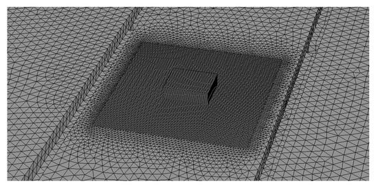
Figure 2.
A sample view of the numerical mesh used in the analysis—structured Cartesian mesh (δx = 0.1 m) in the vicinity of ventilator and area above the fire and unstructured tetrahedral mesh (max. δi = 0.4 m) in the rest of the domain.
The mesh was created following the guidelines presented in [37] and was verified following a mesh sensitivity analysis. For this purpose, one case (fire scenario 2, closed vent) was simulated on three different models. Coarse mesh refers to the case with δx = 0.2 m, medium mesh refers to a case with δx = 0.1 m, and fine mesh refers to a case with δx = 0.05 m in the proximity of the ventilator. It was found that the decrease of mesh size below δx = 0.1 m did not lead to a different outcome in terms of the resulting sprinkler activation time (with the exception of scenarios 12, 24, and 36). On the other hand, increasing the mesh size to δx = 0.2 m resulted in significant differences in activation time for almost all of the scenarios. In consequence, the medium (δx = 0.1 m) mesh was chosen for the rest of the analyses as the best compromise between the quality and the numerical costs. The results of the sensitivity analysis are summarized in Figure 3.
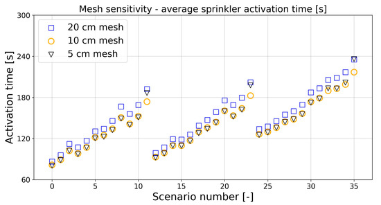
Figure 3.
Activation time for different scenarios for three types of mesh investigated in the mesh sensitivity study.
5. Results and Discussion
Six simulations were performed in which three fire scenarios (fires 1–3) and two conditions of the ventilation system (vents closed or open) were used.
For each of the six scenarios, 36 combinations of sprinkler parameters (Table 2) were assessed, resulting in the overall creation of 216 individual sprinkler activation time maps. A subset of these scenarios was chosen to present the visual results of the analysis in this paper. The complete set of data underwent a quantitative investigation based on the average, maximum, and minimum values of activation time recorded at 600th second of the simulation in cells located within a 6 × 6 × 1 m volume situated near the source of fire and the nearest vent, as shown in Figure 4.
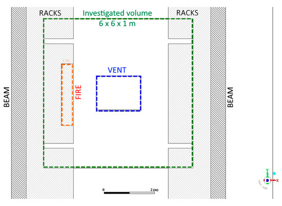
Figure 4.
Illustration (top view) of the part of the numerical model used in the post-processing of the results and statistics.
The results of the calculation with the novel approach can be presented in the form of a 3D activation map. Figure 5 shows an example of such map that was created with the iso-surfaces of sprinkler activation times of 60, 120, and 180 s for fire scenario 2, sprinklers with Tact = 68 °C, Tact = 92 °C, Tact = 141 °C, and Tact = 182 °C (in all cases RTI = 20, C = 1). The iso-surface approach is useful to determine the optimal size of a sprinkler grid in order to meet a target goal of activation time (and, to some extent, the target heat release rate of the fire). In the case of the results shown in Figure 5, the closed vent scenario should be considered as the basic results (the vent has no significant effect on the results). Comparing the results for the closed and open vents, it could be observed that the iso-surfaces for open vents were skewed to one side as an effect of flow within the compartment. Furthermore, the iso-surfaces for open vent scenarios cover less of the volume. This indicates a negative effect of the vents on sprinkler activation. The iso-surface plots provide good visual indication of sprinkler activation; however, their use is mostly limited to qualitative analysis.
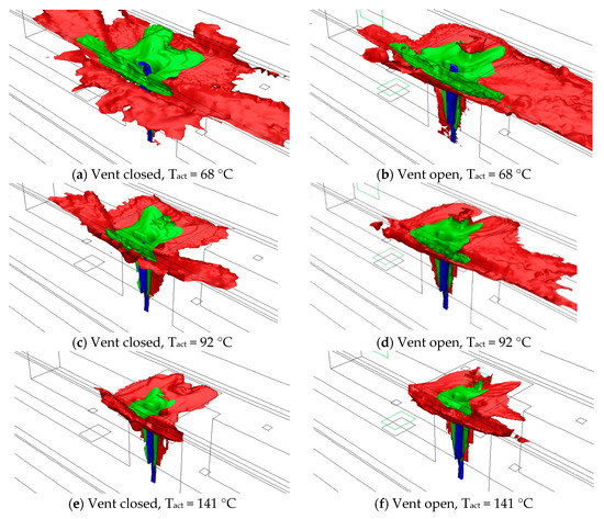
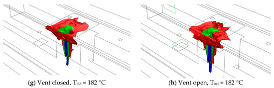
Figure 5.
3D sprinkler activation time maps—iso-surfaces of sprinkler activation in 60 s (red), 120 s (green), and 180 s (blue) from the ignition of the fire. Calculations for fire scenario 2, and the domain area shown in Figure 3.
Quantitative result analysis was possible through activation time statistics in chosen parts of the analyzed domain, as shown in Figure 6 and Figure 7. This allowed for a more robust assessment of the effects of vents or architectural barriers on sprinkler activation, within a pre-defined area of the space. Figure 6 presents the results of the average activation time within the volume defined in Figure 4 for each fire scenario and different values of the RTI and C parameters. The circles represent average values for the scenarios in which the vents were partially open, while triangles represent values for scenarios in which the vents were closed. As expected, the average activation time increased with both the increase in nominal sprinkler activation temperature (Tact) and the RTI value of the sprinkler. In the scenarios with a faster growth of fire and a higher heat release rate, the average time for sprinkler activation was shorter than for slower and smaller fires. In case of 68 °C sprinklers (RTI = 20 and C = 1), the average activation times of sprinklers in a closed vents scenario were 164, 89, and 75 s for fires 1, 2, and 3, respectively. What was noticeable was that the differences between cases with different C constants were larger when the sprinkler activation temperature was higher.
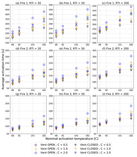
Figure 6.
Average time of sprinkler activation (s) within the predefined region (Figure 4) for all performed simulations. Different plots (a–i) represent different Fire scenarios (1–3) and different RTI values (20, 50 and 200), as described in the title above each plot
Figure 7.
The percentage of the numerical cells in which the activation of sprinkler occurred within the simulation time (600 s) for different fire sources, response time index (RTI) and C values. Different plots (a–i) represent different Fire scenarios (1–3) and different RTI values (20, 50 and 200), as described in the title above each plot.
Open ventilators obviously impact the flow of heat and mass in the smoke layer and, consequently, the sprinkler activation time. However, for the first time, this effect was quantified within a predefined volume (and not just at one particular point in space). For the 68 °C sprinklers (RTI = 20 and C = 1), the average activation times in simulations with partially open vents were longer by 15%, 13%, and 9% for fire scenarios 1, 2, and 3, respectively. This difference was shown to be larger for sprinklers with a higher activation temperature. For 141 °C sprinklers (RTI = 20 and C = 1), the average times of activation for fire scenarios 1, 2, and 3 in simulations with partially open vents were longer by 23%, 19%, and 10%, respectively, and for 182 °C sprinklers (RTI = 20 and C = 1) by 28%, 27%, and 17%, respectively. The highest difference in the average activation time between corresponding cases with open and closed vent was 40%, and it was noted for fire scenario 2 for 182 °C sprinklers (RTI = 200 and C = 2).
Furthermore, the novel approach allowed for the assessment of the statistics of the number of sprinklers activated within a defined region in terms of the percentage of cells in which the sprinklers would have activated. A 100% sprinkler activation meant that a sprinkler would activate within the time of simulation, located in any given place within the analyzed volume. The results of this calculation are shown in Figure 7. It can be concluded that for most of the cases with a closed vent (excluding Tact = 182 °C, RTI = 20–200, C = 1–2), the sprinklers would have activated in all of the cells within the predefined region for all fire scenarios. A similar conclusion may be formed for the cases with open vents and low-temperature sprinklers (Tact = 68 °C and Tact = 92 °C). As shown in Figure 7, some differences can be found in the time of activation; however, the smoke venting did not prevent the sprinkler operation. In case of high-temperature sprinklers (Tact = 141 °C and Tact = 182 °C), a significant number of devices (12%–61%) were not activated within the duration of the simulation (10 min). This can be interpreted as a significant effect of venting action on sprinkler performance, especially on the sprinklers located further away from the fire (e.g., the second row of sprinklers). In many performance-based design projects, the activation of such sprinklers is considered necessary for controlling the size of the fire. If the activation of the second row is delayed, the fire may grow to a size that exceeds the control capacity of the sprinkler system.
A more detailed spatial investigation of the sprinkler activation events was possible with the use of 2D activation maps. Figure 8 presents comparison of sprinkler activation time in a plot 20 cm under the ceiling for fire scenario 2 and Tact = 68 °C, Tact = 141 °C, and Tact = 182 °C sprinklers (all RTI = 20, C = 1). In this plot, it can be observed that the existence of the vent itself disturbed the flow of the ceiling jet, and, in consequence, the activation time was not symmetrical, as it would be if it were obtained with simple hand calculations.
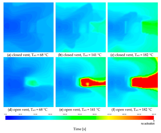
Figure 8.
2D plots of sprinkler activation time 20 cm underneath the ceiling in the region described in Figure 4. Results for fire scenario 2.
Furthermore, the partially open vent had a significant effect on the activation of the link under the vent. This observation raised some concerns, as many vents use trigger mechanisms to automatically switch from “comfort mode” to “fire mode.” If this operation is delayed, the venting action may not be as efficient as the designer expects. This potentially dangerous condition of the system can be efficiently detected with the novel approach, and mitigating measures can be taken.
The designer choosing the applicable location for sprinklers usually relies on their intuition and the standard requirements, which vaguely regulate the location of sprinklers versus obstacles. Alternatively, existing CFD codes allow for the individual assessment of sprinkler activation at a given location, which allows for the optimization of the location, albeit with a costly iterative approach. Conversely, the proposed use of a 3D mapping approach allows for the determination of the best locations for sprinklers in a single iteration for each design fire location.
6. Conclusions
A novel implementation of a well-known empirical model of sprinkler activation (RTI) into the numerical scheme of the general-purpose CFD code ANSYS Fluent has been introduced. This allows for a seamless calculation of sprinkler activation time within each discrete cell of the numerical domain, as well as the further presentation of the data in the form of a 3D activation map, 2D plots, and surface and volumetric statistics. These forms of presentation improve the readability of the results and allow for the optimized positioning of sprinklers against architectural elements or vents. The proposed method may find extensive use in fire safety practice in order to determine the effects of various systems (ventilation, compartmentation) or building architecture on the activation of sprinklers. However, for such use, the implementation of the method in ANSYS Fluent code requires further detailed validation.
The application of the novel approach was demonstrated with a case study of an industrial building that was equipped with natural vents in comfort mode. The results confirmed that the size of the fire and the sprinkler activation temperature were the most important user-defined variables that affect sprinkler activation time. It was observed that the effects of the RTI value and the C parameter were less important for low-temperature sprinklers (68 and 92 °C) and moderately important for high-temperature sprinklers. The new modelling approach confirmed that the common strategy of using high-temperature actuators for vents seems feasible to safely delay vent operation. Furthermore, a unique observation that was made possible by the 3D mapping approach was the lack of sprinkler activation in the middle point of the partially open natural ventilator. This indicates that a vent operating in day-to-day comfort ventilation mode may fail to switch its operation mode in a fire.
As demonstrated in the case study, the effects of ventilation of a compartment on sprinkler activation pattern and activation time can be significant. The sole existence of the vent (even when it was closed) affected the ceiling jet and, in consequence, the sprinkler activation time. In case of open vents, the airflow pattern in the domain influenced the ceiling jet direction, possibly altering the sprinkler operation pattern. Partially open vents delayed sprinkler operation in scenarios of large fires, and the average delay was between 9% and 40%. In some cases, the vents reduced the number of cells in which sprinkler activation would occur up to 40% of the analyzed part of the domain. Numerous findings related to the negative effect of vent operation on sprinkler activation obtained from a simple case study demonstrate the versatility and new research capabilities introduced by the novel approach.
Author Contributions
Conceptualization, W.W., W.J., A.K. and M.K.; data curation, G.K. and A.K.; formal analysis, A.K.; Investigation, W.W., P.T., W.J. and M.K.; methodology, W.W., G.K., P.T. and W.J.; Software, A.K.; supervision, P.T. and M.K.; validation, A.K.; visualization, W.W.; writing—original draft, W.W., W.J., A.K. and M.K.; writing—review and editing, W.W., P.T., W.J. and M.K. All authors have read and agreed to the published version of the manuscript.
Funding
This research received no external funding.
Conflicts of Interest
The authors declare no conflict of interest.
References
- NFPA. NFPA 13, Standard for the Installation of Sprinkler Systems; NFPA: Quincy, MA, USA, 2019. [Google Scholar]
- VdS. VdS 2815en: 2013-09 Interaction of Water Extinguishing Systems and Smoke and Heat Exhaust Ventilation Systems (SHEVS); VdS: Cologne, Germany, 2013. [Google Scholar]
- Heskestad, G.; Bill, R.G. Quantification of thermal responsiveness of automatic sprinklers including conduction effects. Fire Saf. J. 1988, 14, 113–125. [Google Scholar] [CrossRef]
- Heskestad, G.; Smith, H.F. Investigation of a New Sprinkler Sensitivity Approval Test: The Plunge Test, FMRC 22485; Factory Mutual Research Corporation: Norwood, MA, USA, 1976. [Google Scholar]
- Croce, P.; Beyler, C.; Dubay, C.; Johnson, P.; McNamee, M. Fast-Response Sprinkler Technology: Hsiang-Cheng Kung, Gunnar Heskestad, Robert Bill, Roger Allard: The 2019 Phillip J. DiNenno Prize. Fire Technol. 2020. Available online: https://link.springer.com/article/10.1007/s10694-020-00961-7#article-info (accessed on 19 March 2020).
- Pepi, J.S. Design Characteristics of Quick Response Sprinklers; Grinnel Fire Protection Systems Co: Providence, RI, USA, 1986. [Google Scholar]
- Thorne, P.F.; Theobald, C.R.; Melinek, S.J. The Thermal Performance of Sprinkler Heads. Fire Saf. J. 1988, 14, 89–99. [Google Scholar] [CrossRef]
- Melinek, S.J. Thermal response of sprinklers—A theoretical approach. Fire Saf. J. 1988, 13, 169–180. [Google Scholar] [CrossRef]
- Frank, K.; Spearpoint, M.; Baker, G.; Wade, C.; Collier, P.; Fleischmann, C. Measuring modified glass bulb sprinkler thermal response in plunge and compartment fire experiments. Fire Saf. J. 2017, 91, 662–670. [Google Scholar] [CrossRef]
- You, W.J.; Ko, G.H.; Ryou, H.S. Investigation of the Thermal Characteristics of a Circular Fusible-Type Sprinkler Using the Energy Transport Equation. Fire Technol. 2016, 52, 1409–1425. [Google Scholar] [CrossRef]
- Evans, D.D.; Stroup, D. Methods to calculate the RTI and Smoke Detector installed below large unobstructed ceilings.pdf. Fire Technol. 1985, 22, 54–65. [Google Scholar] [CrossRef]
- Stroup, D.W.; Evans, D.D. Use of computer fire models for analyzing thermal detector spacing. Fire Saf. J. 1988, 14, 33–45. [Google Scholar] [CrossRef]
- Alpert, R.L. Turbulent Ceiling-Jet Induced by Large-Scale Fires. Combust. Sci. Technol. 1975, 11, 197–213. [Google Scholar] [CrossRef]
- Davis, W.D.; Cooper, L.Y. A computer model for estimating the response of sprinkler links to compartment fires with draft curtains and fusible link-actuated ceiling vents. Fire Technol. 1991, 27, 113–127. [Google Scholar] [CrossRef]
- Wade, C.; Spearpoint, M.; Bittern, A.; Tsai, K.W.H. Assessing the sprinkler activation predictive capability of the BRANZFIRE fire model. Fire Technol. 2007, 43, 175–193. [Google Scholar] [CrossRef]
- Joglar, F.; Mowrer, F.; Modarres, M. A Probabilistic Model for Fire Detection. Fire Technol. 2005, 41, 151–172. [Google Scholar] [CrossRef]
- Tuovinen, H. Validation of ceiling jet flows in a large corridor with vents using the CFD code JASMINE. Fire Technol. 1996, 32, 25–49. [Google Scholar] [CrossRef]
- McGrattan, K.B.; Hamins, A.; Stroup, D.W. NISTIR 6196-1 Sprinkler, Smoke & Heat Vent, Draft Curtain Interaction—Large Scale Experiments and Model Development; NIST: Gaithersburg, MD, USA, 1998.
- Olenick, S.M.; Klassen, M.S.; Roby, R.J. Validation Study of FDS for a High-Rack Storage Fire. In Proceedings of the SFPE 3rd Technical Symposium on Computer Applications in Fire Protection Engineering, Baltimore, MD, USA, 12–13 September 2001. [Google Scholar]
- Bittern, A. Analysis of FDS Predicted Sprinkler Activation Times with Experiments; University of Canterbury: Christchurch, New Zealand, 2004. [Google Scholar]
- Hopkin, C.; Spearpoint, M.; Bittern, A. Using experimental sprinkler actuation times to assess the performance of Fire Dynamics Simulator. J. Fire Sci. 2018, 36, 342–361. [Google Scholar] [CrossRef]
- Hurley, M.J.; Madrzykowski, D. Evaluation of the Computer Fire Model DETACT-QS. In Proceedings of the Performance-Based Codes Fire Safety Design Methods, 4th International Conference Proceedings, Melbourne, Australia, 20–22 March 2002. [Google Scholar]
- Quintiere, J.G.; Wade, C.A. Compartment fire modeling. In SFPE Handbook of Fire Protection Engineering, Fifth Edition; Springer: New York, NY, USA, 2016; pp. 981–995. ISBN 9781493925650. [Google Scholar]
- Merci, B.; Beji, T. Fluid Mechanics Aspects of Fire and Smoke Dynamics in Enclosures; CRC Press: Leiden, The Netherlands; ISBN 9781138029606.
- VDI. VDI 6019 Blatt 1 Ingenieurverfahren zur Bemessung der Rauchableitung aus Gebäuden Brandverläufe, Überprüfung der Wirksamkeit; VDI: Düsseldorf, Germany, 2006. [Google Scholar]
- NFPA. NFPA 92 Standard for Smoke Control Systems 2015 Edition; NFPA: Quincy, MA, USA, 2015. [Google Scholar]
- Tlili, O.; Mhiri, H.; Bournot, P. Empirical correlation derived by CFD simulation on heat source location and ventilation flow rate in a fire room. Energy Build. 2016, 122, 80–88. [Google Scholar] [CrossRef]
- Bari, S.; Naser, J. Simulation of smoke from a burning vehicle and pollution levels caused by traffic jam in a road tunnel. Tunn. Undergr. Sp. Technol. 2005, 20, 281–290. [Google Scholar] [CrossRef]
- Król, A.; Król, M. Study on Hot Gases Flow in Case of Fire in a Road Tunnel. Energies 2018, 11, 590. [Google Scholar] [CrossRef]
- Boroń, S.; Węgrzyński, W.; Kubica, P.; Czarnecki, L. Numerical Modelling of the Fire Extinguishing Gas Retention in Small Compartments. Appl. Sci. 2019, 9, 663. [Google Scholar] [CrossRef]
- Król, A.; Król, M. Transient Analyses and Energy Balance of Air Flow in Road Tunnels. Energies 2018, 11, 1759. [Google Scholar] [CrossRef]
- NFPA. NFPA 204 Standard for Smoke and Heat Venting 2015 Edition; NFPA: Quincy, MA, USA, 2015. [Google Scholar]
- MoBIaE C/VM2 Verification Method: Framework for Fire Safety Design For New Zealand Building Code Clauses C1-C6 Protection from Fire; The Ministry of Business, Innovation and Employment: Wellington, New Zealand, 2014.
- Węgrzyński, W.; Vigne, G. Experimental and numerical evaluation of the influence of the soot yield on the visibility in smoke in CFD analysis. Fire Saf. J. 2017, 91, 389–398. [Google Scholar] [CrossRef]
- Węgrzyński, W.; Krajewski, G. Influence of wind on natural smoke and heat exhaust system performance in fire conditions. J. Wind Eng. Ind. Aerodyn. 2017, 164, 44–53. [Google Scholar] [CrossRef]
- Król, M. Numerical studies on the wind effects on natural smoke venting of atria. Int. J. Vent. 2016, 15, 67–78. [Google Scholar] [CrossRef]
- Węgrzyński, W.; Lipecki, T.; Krajewski, G. Wind and Fire Coupled Modelling—Part II: Good Practice Guidelines. Fire Technol. 2018, 54, 1443–1485. [Google Scholar] [CrossRef]


© 2020 by the authors. Licensee MDPI, Basel, Switzerland. This article is an open access article distributed under the terms and conditions of the Creative Commons Attribution (CC BY) license (http://creativecommons.org/licenses/by/4.0/).