Article

Heat Transport Analysis in Rectangular Shields Using the Laplace and Poisson Equations †

Faculty of Civil Engineering and Geodesy, Military University of Technology, 00-908 Warsaw, Poland
*
Author to whom correspondence should be addressed.
This paper is an extended version of our paper published in 4th Central European Symposium on Building Physics (CESBP 2019), Prague, Czech Republic, 2–5 September 2019; pp. 1–12.
Energies 2020, 13(7), 1714; https://doi.org/10.3390/en13071714
Submission received: 5 February 2020 / Revised: 16 March 2020 / Accepted: 20 March 2020 / Published: 3 April 2020
(This article belongs to the Special Issue Recent Developments in Building Physics)

Abstract

:
In the design of a building envelope, there is the issue of heat flow through the partitions. In the heat flow process, we distinguish steady and dynamic states in which heat fluxes need to be obtained as part of building physics calculations. This article describes the issue of determining the size of those heat fluxes. The search for the temperature field in a two-dimensional problem is common in building physics and heat exchange in general. Both numerical and analytical methods can be used to obtain a solution. Two methods were dealt with, the first of which was used to obtain the solution in the steady state and the other in the transient. In the steady state a method of initial functions, the basics of which were given by W.Z. Vlasov and A.Y. Lur’e was adopted. Originally MIF was used for analysis of the loads of a flat elastic medium. Since then it was used for solving concrete beams, plates and composite materials problems. Polynomial half-reverse solutions are used in the theory of a continuous medium. Here solutions were obtained by the direct method. As a result, polynomial forms of the considered temperature field were obtained. A Cartesian coordinate system and rectangular shape of the plate were assumed. The problem is governed by the Laplace equation in the steady state and Poisson in the transient state. Boundary conditions in the form of temperature (τ(x), t(y)) or/and flux (p(x), q(y)) can be provided. In the steady state the solution T(x, y) was assumed in the form of an infinite power series developed in relation to the variable y with coefficients Cn depending on x. The assumed solution was substituted into the Fourier equation and after expanding into the Taylor series the boundary condition for y = 0 and y = h was taken into account. From this condition the coefficient Cn can be calculated and, therefore, a closed solution for the temperature field in the plate.

1. Introduction

The search for the temperature field in a two-dimensional problem is common in building physics and heat exchange in general. Both numerical and analytical methods can be used to obtain a solution [1,2]. Thermal and moisture diffusion can also be traced by a marker medium present in the specimen [3]. Two methods were dealt with, the first of which was used to obtain the solution in the steady state and the other in the transient. In a steady state a Method of Initial Functions, the basics of which were given by [4,5] were adopted. The approach used in MIF allowed to derive the form of harmonic polynomials, which form the basis of the solutions in this paper. These polynomials are four times infinity, which is the unique value of this article. An important value of this article is the use of these polynomials to determine the temperature in a rectangular area. In the transient state, the integral heat balance method was used. Three sub-areas were distinguished in the heat transport process and the process of transient heat flow was described.
Originally MIF was used for analysis of the loads of a flat elastic medium [6]. Since then it was used for solving concrete beams, plates and composite materials problems [7,8]. A solution in the form of a power series with coefficients depending on x was assumed. Then these coefficients were found by solving the differential equation. Harmonic polynomials were obtained that satisfy the Laplace equation in the area. The coefficients of the linear combination of these functions were determined by approximating the boundary conditions. The values of the approximation function for the edge of the considered area are here initial functions. As a result, polynomial forms of the considered temperature function were obtained.
The task of analyzing temperature states in rectangular areas form the basis of building physics. They are related to the building envelope, external partitions and ceilings. In building design, these tasks are calculated using standard procedures. This is a special topic in the field of building energy demand regarding external partitions. Procedures used in this topic contain simplifications causing these analyses to be subject to significant errors. The main simplification is the replacement of dynamic processes with steady ones. In fact, in building components, depending on the variability of boundary conditions, static and dynamic states alternate [9,10,11]. There is a problem of improving the methods of analyzing heat transfer processes through the building envelope. Solutions to this problem appear in the existing task classes. Task classes can be distinguished by their formulation in the physics of construction.
I.
Because of the boundary conditions:
First, second and third conditions. Fourth type.
II.
Due to cyclical boundary conditions [12]:
Temperature, solar radiation
III.
Due to the number and order of layers of materials in the partition [13,14,15]:
Single-material, multi-layer.
IV.
Due to the type of impulse:
Dirac delta, step Heaviside function.
Each of these classes has rich literature, and it is presented in separate building physics textbooks. In this article, we will deal with the formulation under boundary conditions of the first type, two static and dynamic states occurring between these two states. The original elements of the article are the distribution in a steady state of the temperature into four states due to symmetry with respect to the variables x, y and the application of the condition from integration of the Poisson equation in the scope of the duration of the dynamic process.
The primary concepts are the boundary components, heat transfer flux, governing equation and characteristic operators of the solutions.

2. Materials and Methods

2.1. Governing Equation

The heat transfer equation derived from the energy balance in the infinitesimal volume:
ρ c p T t = x ( λ x x T x ) + y ( λ y y T y ) + q v ,
where T(x, y) is temperature, ρ—density, cp—specific heat capacity, λ—coefficient of thermal conductivity, and qv—internal heat gains.
In the transient state, Equation (1), with the assumption that the coefficient λ does not depend on temperature, takes the form
ρ c p T t = λ ( T 2 2 x + T 2 2 y ) ρ c p T t = λ ( T 2 2 x + T 2 2 y )
In the steady state heat exchange, with no internal heat sources and an isotropic body, Equation (1) becomes
2 T ( x , y ) = 0 2 = ( 2 x 2 + 2 y 2 ) .
In this consideration, expressions were found for the temperature that satisfies the Laplace equation in the area. This solution has the form of a sum of polynomials. These polynomials exist in products with constant coefficients. The obtained solution was divided into four independent states according to the symmetry features of the temperature function. These are the following:
  • symmetry–symmetry SS (x and y even),
  • symmetry–antisymmetry SA (x even, y odd),
  • antisymmetry–symmetry AS (x odd, y even),
  • antisymmetry–antisymmetry AA (x and y odd).

2.2. Boundary Conditions

The coordinate system and geometrical parameters of the medium were assumed as in Figure 1.
The variable t is the set temperature at the edge of the shield (approximated), and variable T is the interior temperature (approximating). The following boundary conditions apply:
y = h U t ( x ) , 2 . y = h L W t ( x ) x = b R t ( y ) . 4 . x = b L F t ( y ) .
Preceding the variable t, the capital letters U, LW, R and LF were assigned as the temperature of the upper, lower, right and left edges, respectively. The task was divided into four independent problems corresponding to four independent thermal states of the symmetry of the shield. The boundary conditions for the entire shield were split over four states specified in the first quadrant of the coordinate system. The following indices have been assigned to shorten the description of these states: The temperature in the SS state is preceded by the letter S, in the SA state with the letter B, the AS with the letter C and in the state AA with the letter A. The boundary conditions in these states are determined by the initial state with the following formulas:
SS state
y = + h , T S = S U t = S L W t = 1 4 [ U t ( x ) + U t ( x ) + L W t ( x ) + L W t ( x ) ] x = + b , T S = S R t = S L F t = 1 4 [ R t ( y ) + R t ( y ) + L F t ( y ) + L F t ( y ) ] .
SA state
y = + h , T B = B U t = B L W t = 1 4 [ [ U t ( x ) + U t ( x ) ] [ L W t ( x ) + L W t ( x ) ] ] x = + b , T B = B R t = B L F t = 1 4 [ R t ( y ) R t ( y ) + [ L F t ( y ) L F t ( y ) ] ] .
AS state
y = + h , T C = C U t = C L W t = 1 4 [ [ U t ( x ) U t ( x ) ] + [ L W t ( x ) L W t ( x ) ] ] x = + b , T C = C R t = C L F t = 1 4 [ [ R t ( y ) + R t ( y ) ] [ L F t ( y ) + L F t ( y ) ] ] .
AA state
y = + h , T A = A U t = A L W t = 1 4 [ [ U t ( x ) U t ( x ) ] [ L W t ( x ) L W t ( x ) ] ] x = + b , T A = A R t = A L F t = 1 4 [ [ R t ( y ) R t ( y ) ] [ L F t ( y ) L F t ( y ) ] ] .
For example, boundary conditions for the whole shield on the lower edge will be equal to the sum S D t ( x ) + B D t ( x ) + C D t ( x ) + A D t ( x ) .
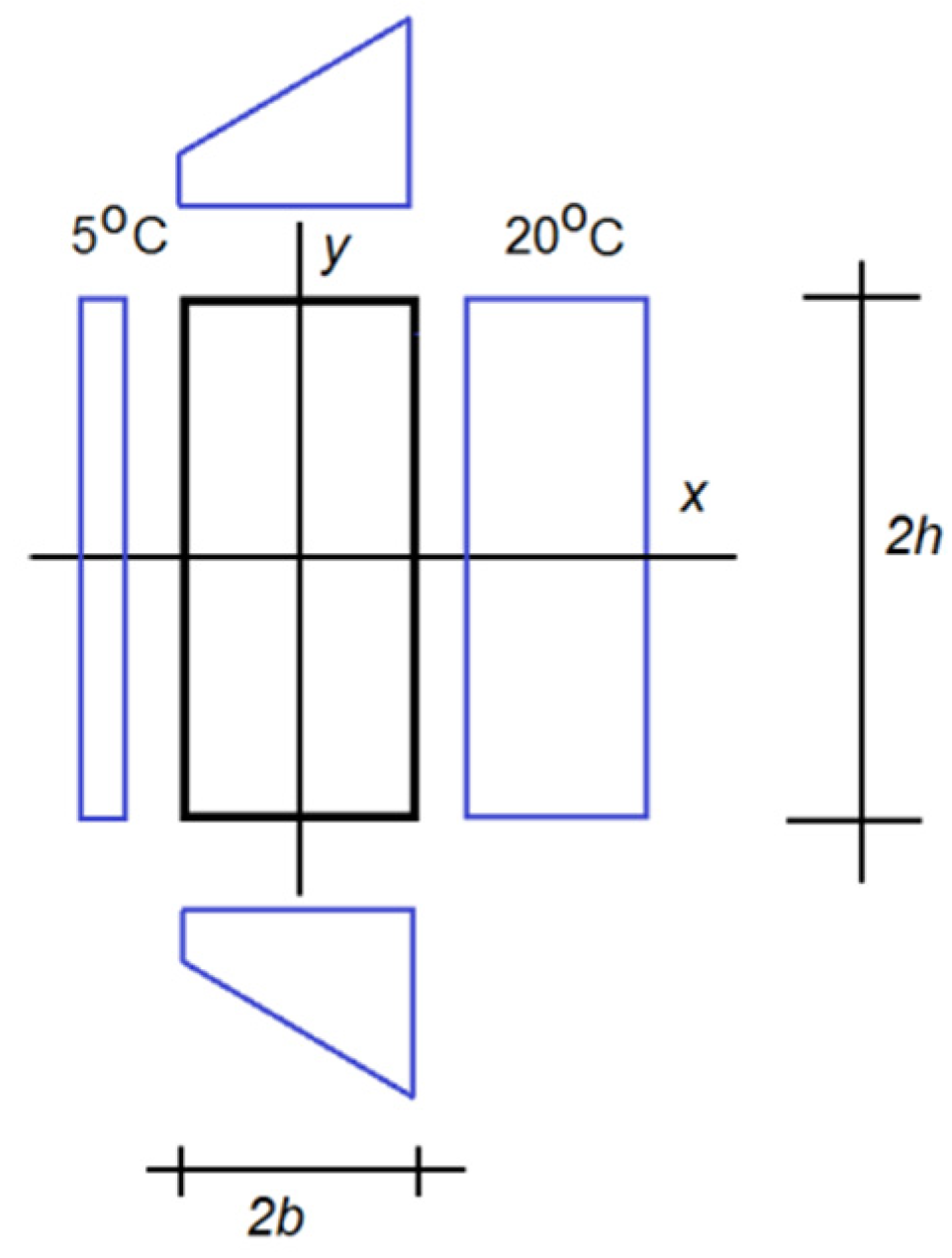
Example. Considering that the element has a geometry as in Figure 2.
Assuming an outside temperature of 5 °C and inside temperature of 20 °C, the boundary conditions for the steady state can be described by the following functions:
y = + h T = U t = L W T = 5 + 15 2 b ( b + x ) , x = + b T = R t = 20 ° C L F T = 5 ° C
The graphical representation of boudry conditions can be found on Figure 3
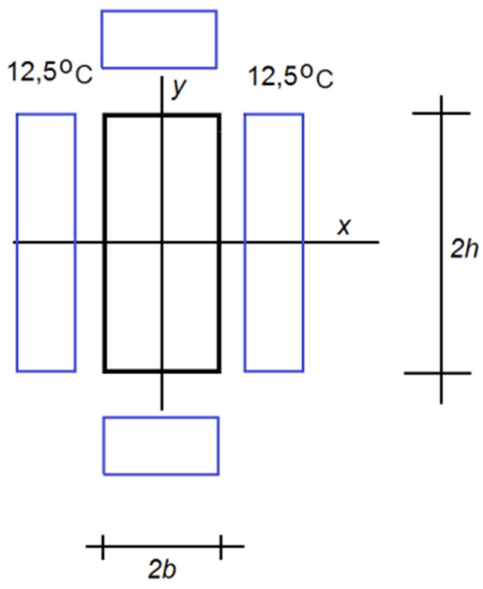
The task is split into four states using Equations (4)–(7): The boundary conditions in the SS and AS states are shown in Figure 4 and Figure 5.
SS state
y = + h T S = S U t = S L W t = 1 4 [ 5 + 15 2 b ( b + x ) + 5 + 15 2 b ( b x ) + 5 + 15 2 b ( b + x ) + 5 + 15 2 b ( b x ) ] = 12.5 ° C x = + b T S = S R t = S L F t = 1 4 ( 20 + 20 + 10 + 10 ) = 12.5 ° C
AS State
y = + h T C = C U t = C L W T = 1 4 [ ( 5 + 15 2 b ( b + x ) 5 15 2 b ( b x ) ) + ( 5 + 15 2 b ( b + x ) 5 15 2 b ( b x ) ) ] = 15 x 2 b , x = + b T c = C R t = 1 4 ( 20 + 20 5 5 ) = 7.5 ° C C L F T = 7.5 ° C
The SA and AA states are identically zero:
y = + h T S A = T A A = C U t = C L W T = 0 ° C x = + b T S A = T A A = C R t = C L F t = 0 ° C

2.3. Solution of the Area Problem in Steady State

The solution functions T(x, y) were assumed in the form of an infinite power series developed in relation to the variable y with coefficients Cn depending on x.
T ( x , y ) = n = 0 C n ( x ) y n .
Second derivatives with respect to x:
2 T x 2 = n = 0 2 C n ( x ) x 2 y n ,
and with respect to y:
2 T y 2 = n = 2 ( n 1 ) n C n ( x ) y ( n 2 ) ,
were calculated. The substitution n = n + 2 was performed to Equation (14) where n is a new variable with the same designation and Equation (14) was rewritten in the form
2 T y 2 = n = 0 ( n 1 ) ( n + 2 ) C n + 2 ( x ) y n .
After substituting Equations (13) and (15) in (2b)
n = 0 2 C n ( x ) x 2 y n + n = 0 ( n 1 ) ( n + 2 ) C n + 2 ( x ) y n = 0 .
Cn(x) are treated as n-dependent terms of progression and as such can be derived from the differential Equation (16). Putting the sum into a common sign and introducing the operator D:
n = 0 [ C n + 2 ( n + 2 ) ( n + 1 ) + D 2 C n ] y n = 0 ,
where D n = n x n .
Equation (17) will be met if
C n + 2 ( n + 2 ) ( n + 1 ) + D 2 C n = 0 .
Multiplying both sides by (n!/n!) a differential equation on Cn(x) is obtained:
C n + 2 ( n + 2 ) ! n ! + D 2 C n n ! n ! = 0 .
After applying the shift operator
E p C n = C n + p ,
[ E 2 + D 2 ] C n n ! = 0 .
Equation (21) can be solved as an equation with constant coefficients; the general solution is
C n n ! = ( i D ) n A + ( i D ) n B .
Variables A and B were determined by substituting n = 0, 1 for Equation (22). In this way expressions were obtained on C0 and C1, although their value is unknown, one can express A and B:
C o = A + B C 1 = i D A + i D B
Determining A and B from Equation (23), the following was obtained:
A = 1 2 [ C 0 ( i D ) 1 C 1 ] B = 1 2 [ C 0 + ( i D ) 1 C 1 ]
Substituting Equations (24) to (22) and introducing divalent functions j(n), j(n + 1) with values (0,1)
j ( n ) = 1 2 [ ( 1 ) n + 1 ] , j ( n + 1 ) = 1 2 [ 1 + ( 1 ) n + 1 ] ,
and trivalent J(n) and J(n + 1) with values (−1, 0, +1)
J ( n ) = j ( n ) i n , J ( n + 1 ) = j ( n + 1 ) i n + 1 ,
an expression for Cn term is as follows
C n = 1 n ! [ J ( n ) D n C o J ( n + 1 ) D n 1 C 1 ] .
Substituting Equations (27) to (12)
T ( x , y ) = n = 0 1 n ! [ J ( n ) D n C o J ( n + 1 ) D n 1 C 1 ] y n .
The Taylor series expansion of the sin() and cos() function is
cos D y = n = 0 J ( n ) ( D y ) n n ! , sin D y = n = 0 J ( n + 1 ) ( D y ) n n ! .
Equation (28) can be written in the form
T ( x , y ) = cos D y C o + sin D y D C 1 .
Separating Equation (30) into a symmetrical and antisymmetrical part relative to the variable y, we obtained
X S T ( x , y ) = cos D y T ( x , 0 ) = cos D y i = 0 T i x i
X A T ( x , y ) = sin ( D y ) D C ( x , 0 ) = sin ( D y ) D i = 0 C ˙ i x i ,  
XS before the function T(x, y) means that the function T(x, y) is arbitrary with respect to x and even with respect to y, likewise the designation XA means that the function T(x, y) is odd in relation to the variable y. Taking into account in Equations (31) and (32) the relationship j(i) + j(i + 1) = 1 as well as Equation (29), the following were obtained:
X S T ( x , y ) = i = 0 ( [ j ( i ) + j ( i + 1 ) ] T i k = 0 i J ( k ) ( k i ) x i k y k )
X A T ( x , y ) = i = 0 ( [ j ( i ) + j ( i + 1 ) ] C i k = 0 i + 1 J ( k + 1 ) ( k i + 1 ) x i + 1 k y k ) .
Equations (33) and (34) can be easily separated into state symmetry–symmetry (SS), symmetry–antisymmetry (SA), antisymmetry–symmetry (AS) and antisymmetry–antisymmetry (AA). The temperature in individual states is expressed in the following formulas:
SS state
S S T ( x , y ) = i = 0 ( j ( i ) T i k = 0 i J ( k ) ( i k ) x i k y k ) ,
AS state
A S T ( x , y ) = i = 0 ( j ( i + 1 ) T i k = 0 i J ( k ) ( i k ) x i k y k ) ,
SA state
S A T ( x , y ) = i = 0 ( j ( i ) C i k = 0 i + 1 J ( k + 1 ) ( i + 1 k ) x i + 1 k y k ) ,
AA state
A A T ( x , y ) = i = 0 ( j ( i + 1 ) C i k = 0 i + 1 J ( k + 1 ) ( i + 1 k ) x i + 1 k y k ) .
The polynomials specified in Equations (35)–(38) are harmonics, i.e., they satisfy the Laplace equations. By accepting a sufficient number of polynomials and their corresponding constant factors, boundary conditions can be met precisely enough.
In this work, the method of approximating the temperature at the edges of the shield was used to determine the constant coefficients.

2.4. Expressions on Temperature in Case of Limitation to the First Consecutive Polynomials of Rank 10

Equations (35)–(38) contain an infinite number of constant factors and an infinite number of polynomials corresponding to these coefficients. In specific calculations, the number of these coefficients and the corresponding degrees of polynomials can be limited. The values of functions j(n), J(n) necessary to write the equations are summarized in Table 1.
The following are given in individual states of temperature symmetry: five polynomials corresponding to the following “n” rank: SS—8, SA—9, AS—9 and AA—10.
SS state
T ( x , y ) = T o + T 2 ( x 2 y 2 ) + T 4 ( x 4 6 x 2 y 2 + y 4 ) + T 6 ( x 6 15 x 4 y 2 + 15 x 2 y 4 y 6 ) + + T 8 ( x 8 28 x 6 y 2 + 70 x 4 y 4 28 x 2 y 6 + y 8 ) , ,
AS state
T ( x , y ) = T 1 x + T 3 ( x 3 3 x y 2 ) + T 5 ( x 5 10 x 3 y 2 + 5 x y 4 ) + + T 7 ( x 7 21 x 5 y 2 + 35 x 3 y 4 7 x y 6 ) + T 9 ( x 9 36 x 7 y 2 + 126 x 5 y 4 84 x 3 y 6 + 9 x y 8 ) ,
SA state
T ( x , y ) = C 1 y + C 3 ( 3 x 2 y y 3 ) + C 5 ( 5 x 4 y 10 x 2 y 3 + y 5 ) + + C 7 ( 7 x 6 y 35 x 4 y 3 + 21 x 2 y 5 y 7 ) + C 9 ( 9 x 8 y 84 x 6 y 3 + 126 x 4 y 5 36 x 2 y 7 + y 9 ) ,
AA state
T ( x , y ) = C 2 x y + C 4 ( x 3 y x y 3 ) + C 6 ( x 5 y 10 x 3 y 3 + 3 x y 5 ) + + C 8 ( x 7 y 7 x 5 y 3 + 7 x 3 y 6 x y 7 ) + C 10 ( 5 x 9 y 60 x 7 y 3 + 126 x 5 y 5 60 x 3 y 7 + 5 x y 9 ) .
As can be seen, these polynomials can be easily written, because their coefficients are equivalents from the Pascal triangle.

3. Results and Discussion

3.1. Solution to the Example Formulated in Point 2

We solve the task of meeting boundary conditions assuming fixed temperatures at the edges x = b; T = tz, y = h; T = τ as in Figure 3. This is the symmetric part of Example.
We adopt the harmonic functions
H o = 1 , H 2 = x 2 y 2 .
Assuming an approximating function in the form
T = a 1 + a 2 ( x 2 y 2 ) .
This function on the right edge takes the form
x = b T p = a 1 + a 2 ( b 2 y 2 ) y = h T g = a 1 + a 2 ( x 2 h 2 )
We will set parameters a1, a2 from the approximation condition; meeting the minimum deviation on the right and upper edges. The minimum deviation condition has the form
min a 1 , a 2 δ = 0 h d y [ a 1 + a 2 ( b 2 y 2 ) t ] 2 + 0 b d x [ a 1 + a 2 ( x 2 h 2 ) τ ] 2 = = 0 h d y { [ a 1 + a 2 ( b 2 y 2 ) ] 2 2 [ a 1 + a 2 ( b 2 y 2 ) ] + t 2 } + 0 h d x { [ a 1 + a 2 ( x 2 h 2 ) ] 2 2 [ a 1 + a 2 ( x 2 h 2 ) ] + τ 2 } = = 0 h d y { [ a 1 2 + 2 a 1 a 2 ( b 2 y 2 ) + a 2 2 ( b 2 y 2 ) 2 ] 2 [ a 1 + a 2 ( b 2 y 2 ) ] t 2 + t 2 } + + 0 h d x { [ a 1 + 2 a 1 a 2 ( x 2 h 2 ) ] + a 2 2 ( x 2 h 2 ) 2 2 [ a 1 + a 2 ( x 2 h 2 ) τ ] + τ 2 } .
Calculating the definite integral, we get
min δ a 1 , a 2 = a 1 2 h + 2 a 1 a 2 ( b 2 h h 3 3 ) + a 2 2 ( b 4 h 2 b 2 h 3 3 + h 5 5 ) 2 ( a 1 h + a 2 ( b 2 h h 3 3 ) ) t + t 2 h + + a 1 2 b + 2 a 1 a 2 ( b 3 3 h 2 b ) + a 2 2 ( b 5 5 2 b 3 3 h 2 + h 4 b ) 2 ( a 1 b + a 2 ( b 3 3 h 2 b ) ) τ + τ 2 b .
By calculating derivatives relative to a1 and a2, we obtained
δ a 1 = a 1 · 2 ( h + b ) + 2 a 2 [ h b ( b h ) + 1 3 ( b 3 h 3 ) ] 2 ( h t b τ ) δ a 2 = a 1 · 2 [ ( b 2 h h 2 b ) + 1 3 ( b 3 h 3 ) ] + 2 a 2 ( b 4 h b h 4 ) + 2 3 ( b 2 h 3 + b 3 h 2 ) + 1 5 ( b 5 + h 5 ) 2 ( h b 2 1 3 h 3 ) t + 2 ( b h 2 1 3 b 3 ) τ .
By equating derivatives to zero, two equations were obtained to determine the a1, a2 constants:
a 1 A 11 + a 2 A 12 = P 1 a 1 A 21 +   a 2 A 22 = P 2
where
A 11 = 2 ( h + b ) , A 12 = A 21 = 2 [ h b ( b h ) + 1 3 ( b 3 h 3 ) ] A 22   = 2 [ ( b 4 h + b h 4 ) 2 3 ( b 2 h 3 + b 3 h 2 ) + 1 5 ( b 5 + h 5 ) ] P 1 = 2 ( h t + b τ ) , P 2   = 2 ( h b 2 1 3 h 3 ) t 2 ( b h 2 1 3 b 3 ) τ W 1 = A 22 P 1 A 12 P 2 =   4 ( 2 15 b 5 h + 4 9 b 3 h 3 + 2 3 b h 5 + 4 45 h 6 ) t + 4 ( 2 3 b 5 h + 4 9 b 3 h 3 2 15 b h 5 + 4 45 b 6 ) τ W = A 11 A 22 A 12 A 21 = 4 ( 4 45 b 6 + 8 15 b 5 h + 8 9 b 3 h 3 + 8 15 b h 5 + 4 45 h 6 ) .
Solution of equations:
a 1 = W 1 W = ( 2 15 b 5 h + 4 9 b 3 h 3 + 2 3 b h 5 + 4 45 h 6 ) t + ( 2 3 b 5 h + 4 9 b 3 h 3 2 15 b h 5 + 4 45 b 6 ) τ 4 45 b 6 + 8 15 b 5 h + 8 9 b 3 h 3 + 8 15 b h 5 + 4 45 h 6
a 2 = W 2 W = ( 2 3 b 3 h + 2 3 b h 3 ) t + ( 2 3 b 3 h 2 3 b h 3 ) τ 4 45 b 6 + 8 15 b 5 h + 8 9 b 3 h 3 + 8 15 b h 5 + 4 45 h 6 .
We assume the dimensions of the wall element shown on Figure 2 as 2h = 3 m and 2b = 0.5 m, therefore:
h b = 6 t = τ = 12.5   ° C y = + h T C = C G t = C D t = 12.5 ° C x = + b T c = C P t = C L t = 12.5 ° C a 1 = W 1 W 2 = 47132 5 t 42152 45 t 382036 45 = 382036 45 t 382036 45 = t = τ a 2 = W 2 W = [ 4 · 222 b 4 3 ] t + [ 4 · 222 b 4 3 ] τ [ 4 45 b 6 + 8 15 b 5 6 b + 8 9 b 3 ( 6 b ) 3 + 8 15 b ( 6 b ) 5 + 4 45 ( 6 b ) 6 ] = 0
The boundary condition in the SS state was shown in Figure 4. The temperature field has the form of Equation (45).
AS state
The boundary condition in the AS-state is shown in Figure 5.
y = + h T C = C G t = C D T = 15 x 2 b , x = + b T c = C P t = 7.5 ° C C L T = 7.5 ° C
T ( x , y ) = T 1 x + T 3 ( x 3 3 x y 2 ) + T 5 ( x 5 10 x 3 y 2 + 5 x y 4 ) + + T 7 ( x 7 21 x 5 y 2 + 35 x 3 y 4 7 x y 6 ) + T 9 ( x 9 36 x 7 y 2 + 126 x 5 y 4 84 x 3 y 6 + 9 x y 8 ) .
In general, we can write for the AS state
T ( x , y ) = T 1 H 1 + T 3 H 3 + T 5 H 5 + T 7 H 7 + T 9 H 9 ,
where
H 1 = x , H 3 = x 3 3 x y 2 H 5 = x 5 10 x 3 y 2 + 5 x y 4 H 7 = x 7 21 x 5 y 2 + 35 x 3   y 4 7 x y 6 H 9 = x 9 36 x 7 y 2 + 126 x 5   y 4 84 x 3 y 6 + 9 x y 8 .
We limit the solution of this example to terms H1 and H3:
T ( x , y ) = a 1 H 1 + a 2 H 3 = a 1 x + a 2 ( x 3 6 y 2 x ) .
The boundary conditions are described by the following equations:
y = + h T C = C G t = C D T = 15 x 2 b = F x 2 b , x = + b T c = C P t = 7.5 ° C = t C L T = 7.5 ° C = t , F = 2 t .
where F, t are fixed numbers.
The square of deviation on the right edge is equal to
δ 2 ( p )   = 0 h d y [ a 1 b + a 2 ( b 3 3 b y 2 ) t ] 2 .
The deviation square on the upper edge is
δ 2 ( g ) = 0 b d x [ a 1 x + a 2 ( x 3 3 x h 2 ) F x 2 b ] 2 .
As a criterion of approximation, we accept the minimum sum of deviations:
m i n a 1 , a 2 δ 2 = δ 2 ( p )   + δ 2 ( g ) = 0 h d y [ a 1 b + a 2 ( b 3 3 b y 2 ) t ] 2 + 0 b d x [ a 1 x + a 2 ( x 3 3 x h 2 ) F x 2 b ] 2 .
Hence the deviation derivatives relative to a1 and a2 are equal to zero:
W a 1 = 0 , W a 2 = 0 , W = 0 h d y [ a 1 b + a 2 ( b 3 3 b y 2 ) t ] 2 + 0 b d x [ a 1 x + a 2 ( x 3 3 x h 2 ) F x 2 b ] 2 .
W a 1 = 0 , W = 0 h d y [ a 1 b + a 2 ( b 3 3 b y 2 ) t ] 2 + 0 b d x [ a 1 x + a 2 ( x 3 3 x h 2 ) F x 2 b ] 2 W a 1 = 0 h d y 2 [ a 1 b + a 2 ( b 3 3 b y 2 ) t ] b + 0 b d x 2 [ a 1 x + a 2 ( x 3 3 x h 2 ) F x 2 b ] x = 0 W a 1 = 2 [ a 1 b h + a 2 ( b 3 h 3 b h 3 3 ) t h ] b + 2 [ a 1 b 3 3 + a 2 ( b 5 5 3 b 3 3 h 2 ) F b 3 b 6 ] = 0   W a 1 = a 1 ( b 2 h + b 3 3 ) + a 2 ( b 4 h 3 b 2 h 3 3 3 b 3 3 h 2 + b 5 5 ) t h b + ( F b 2 6 ) = 0 .
W a 2 = 0 , W = 0 h d y [ a 1 b + a 2 ( b 3 3 b y 2 ) t ] 2 + 0 b d x [ a 1 x + a 2 ( x 3 3 x h 2 ) F x 2 b ] 2 W a 2 = 2 0 h d y [ a 1 b + a 2 ( b 3 3 b y 2 ) t ] ( b 3 3 b y 2 ) + 0 b d x [ a 1 x + a 2 ( x 3 3 x h 2 ) F x 2 b ] ( x 3 3 x h 2 ) = a 1 ( b 5 5 + b 4 h b 3 h 2 b 2 h 3 ) + a 2 ( b 7 7 + b 6 h 6 5 b 5 h 2 2 b 4 h 3 + 3 b 3 h 4 + 9 5 b 2 h 5 ) t ( b 3 h b h 3 ) F ( b 4 10 b 2 h 2 2 ) .
The equations determining a1 and a2 have the form
W a 1 = a 1 ( b 2 h + b 3 3 ) + a 2 ( b 4 h 3 b 2 h 3 3 3 b 3 3 h 2 + b 5 5 ) t h b + ( F b 2 6 ) = 0 W a 1 = a 1 ( b 5 5 + b 4 h b 3 h 2 b 2 h 3 ) + a 2 ( b 7 7 + b 6 h 6 5 b 5 h 2 2 b 4 h 3 + 3 b 3 h 4 + 9 5 b 2 h 5 ) t ( b 3 h b h 3 ) F ( b 4 10 b 2 h 2 2 ) = 0 .
or in an alternative form
a 1 ( b 2 h + b 3 3 ) + a 2 ( b 4 h 3 b 2 h 3 3 3 b 3 3 h 2 + b 5 5 ) = t h b + F b 2 6 a 1 ( b 5 5 + b 4 h b 3 h 2 b 2 h 3 ) + a 2 ( b 7 7 + b 6 h 6 5 b 5 h 2 2 b 4 h 3 + 3 b 3 h 4 + 9 5 b 2 h 5 ) = t ( b 3 h b h 3 ) + F ( b 4 10 b 2 h 2 2 ) .
We write set of equations in the form
A 11 a 1 + A 12 a 2 = P 1 A 21 a 1 + A 22 a 2 = P 2 A 11 = b 2 h + b 3 3 A 12 = b 4 h 3 b 2 h 3 3 3 b 3 3 h 2 + b 5 5 , P 1 = t h b + F b 2 6 A 21 = b 5 5 + b 4 h b 3 h 2 b 2 h 3 A 22 = b 7 7 + b 6 h 6 5 b 5 h 2 2 b 4 h 3 + 3 b 3 h 4 + 9 5 b 2 h 5 ,   P 2 = t ( b 3 h b h 3 ) + F ( b 4 10 b 2 h 2 2 ) ,
W 1 = P 1 A 22 P 2 A 12 = t 2 35 b 3 h ( b 5 + 35 b h 4 + 14 h 5 ) + F 1 1050 b 4 ( 4 b 5 + 70 b 4 h + 280 b 2 h 3 210 h 5 ) W 2 = A 11 P 2 A 21 P 1 = b 4 h 15 ( b 2 + 5 h 2 ) ( 2 t F ) W = A 11 A 22 A 12 A 21 = 4 b 4 525 ( b 6 + 10 b 5 h + 70 b 3 h 3 + 210 b h 5 + 105 h 6 )
a 1 = W 1 W = = 60 t b 2 h ( b 5 + 35 b h 4 + 14 h 5 ) + F b 3 ( 4 b 5 + 70 b 4 h + 280 b 2 h 3 210 h 5 ) 8 ( b 6 + 10 b 5 h + 70 b 3 h 3 + 210 b h 5 + 105 h 6 ) a 2 = W 2 W = 35 b 3 h ( b 2 + 5 h 2 ) ( 2 t F ) 4 ( b 6 + 10 b 5 h + 70 b 3 h 3 + 210 b h 5 + 105 h 6 ) .
For the considered wall dimensions
A 11 = 0.098958 A 12 = 0.24004 A 22 = 1.062973 P 1 = 2.96875 P 2 = 7.20117 W = 4 3 96 35 16 25 = 528 175 = 0.047571 W 1 = 1.427137 W 2 = 0 , a 1 = 30 a 2 = 0
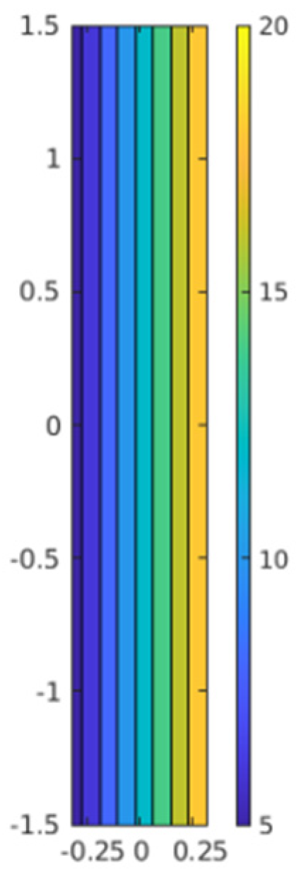
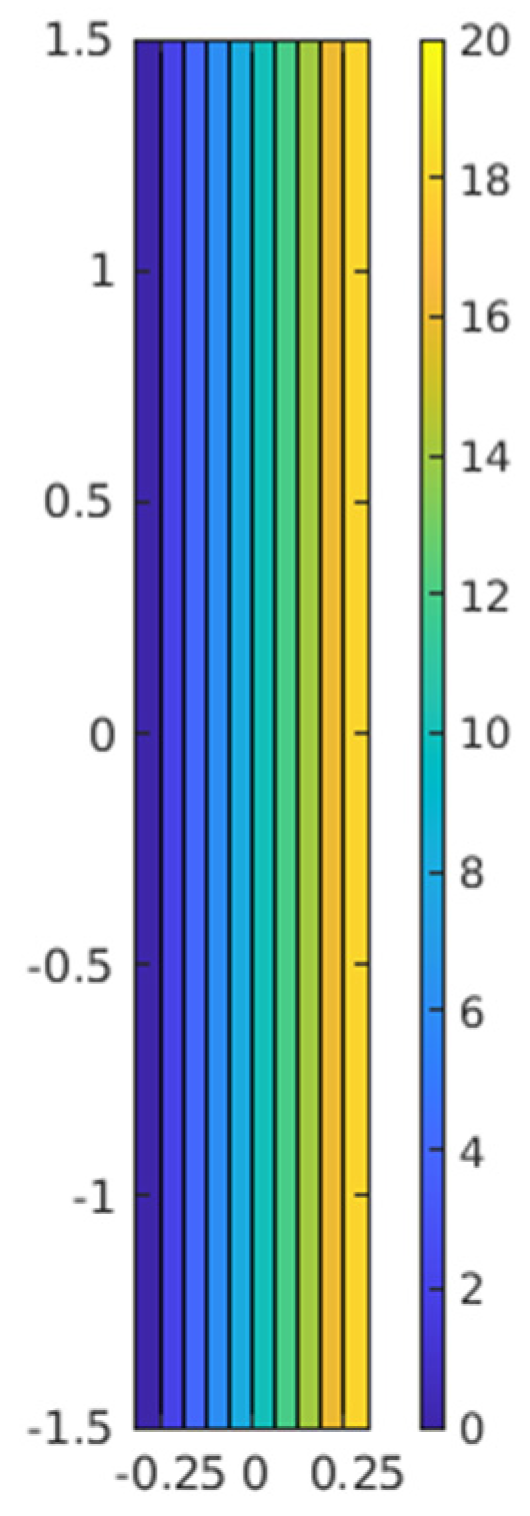
The temperature field has the form
T ( x , y ) = a 1 H 1 = a 1 x = 30 x .
and is shown on Figure 6.
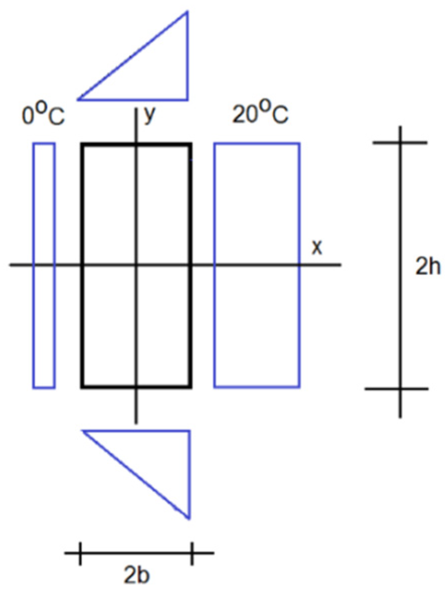
The obtained solution is called the steady state number one. For the completeness of the task we will analyse the second steady state. The temperature on the left bank has been reduced by 5 °C and boundary conditions became as in Figure 7.
By solving the state presented in the drawing, we receive functions similarly to the first example.
State SS T S S ( x , y ) = 10 State AS T A S ( x , y ) = 40 x .
The resulting temperature in the wall in the second state is shown in Figure 8.
It was called the steady state number two.

3.2. Area Solution for Transient State

This section is divided into subheadings to provide a concise and precise description of the experimental results, their interpretation as well as the experimental conclusions that can be drawn.

3.2.1. Task Formulation

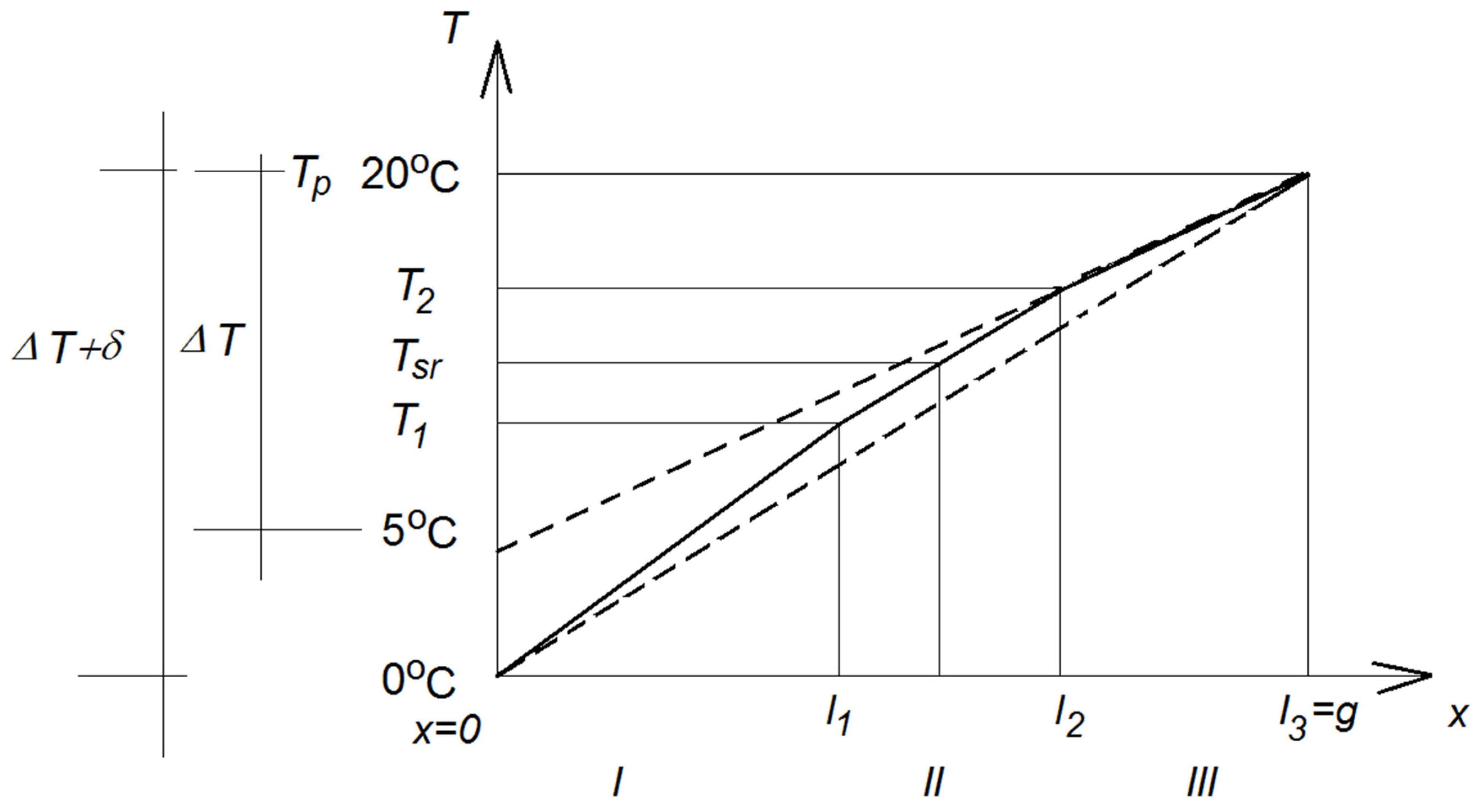
Geometry parameters and boundary conditions of the formulated problem are in Figure 9.
In this part, the process of transition from steady state one to steady state two was studied. In the process, the temperature at the edges is 20 °C and 5 °C, the temperature difference is 15 °C. In the second steady state, the temperature is 20 °C and 0 °C, and the temperature difference is 20 °C.
After the occurrence of the dt pulse, the transition to the second steady state follows. In this range, the temperature change along the x-axis depends on the time measured by the distance from the pulse. This temperature can be visualized with isochrones its course for a given time. The task of determining a representative isochrone for the entire dynamic process was considered.
Dynamic parameters, such as specific heat cp, thermal conductivity λ and density ρ are needed to describe the process.
The left edge of the rectangular wall element is shown in Figure 6, with an initial temperature of 5 °C cooled to 0 degrees by means of an external setting pulse. Cooling is carried out with air at 0 °C. Dimensions: 2a = 0.5 m and 2h = 3 m. The heat transfer coefficient on the surface is 15 W/(mK). Thermal properties of the material: cp = 800 J/(kgK), ρ = 2000 kg/m3 and λ = 1 W/(mK). Cooling time was calculated using the ordered state method [16]. Surface area in the direction of heat flow S = 6 m2 and volume is V = 1.5 m3.
Characteristic dimension
l v = 1.5 3 = 0.5 .
Biot number
B i = α l v λ = 15 × 0.5 1 = 7.5 .
Kondratiew number
K n = B i B i 2 + 1.437 × B i + 1 = 7.5 7.5 2 + 1.437 × 7.5 + 1 = 7.5 68.03 = 0.909 .
Wall thermal diffusivity
a = 1 2000 × 800 = 6.25 × 10 7 ( m 2 s ) .
Cooling rate
m = 6.25 × 10 7 0.5 2 0.909 = 2.273 × 10 6 ( 1 s ) .
Cooling time
e m t = T p T f T k T f = 5 50 0 50
m t = ln ( 5 50 0 50 ) t = 46353   s 12.9   ( h ) .
Fourier number
F o = a t l v = 6.25 × 10 7 × 46353 0.5 2 = 0.12 .
The ordered state theory can be used with an accuracy of 2% [16] if the Fo number is greater than 0.16, so in this case the error is acceptable.
We describe the temperature distribution in the transient process.
Assumptions. The x, y coordinate system. We have a homogeneous band with respect to the spatial coordinate y. There is a temperature difference relative to the coordinate x Δ T = c o n s t . between the right and left edges.

3.2.2. Description of the Temperature Effect Caused by the Pulse on the Left Bank δ T

We assume the temperature rise setting at the left bank by δ T . We do not change the temperature on the right bank. We study the process of temperature propagation at time t along the x coordinate. We use a solution for a temperature pulse on the outer wall of the size δ . The temperature function under boundary conditions of the first type has the following form [17]:
δ T ( x ) = δ ( 1 x d ) 2 .
where d is the distance of the heat diffusion front of the pulse and x is the current coordinate of the temperature diagram. This case corresponds to heat shock on the surface of a flat wall insulated on its own. When the surface temperature is constant, then the relationship between the range of the pulse d and time t is obtained:
d = 3.464 a t .
Coordinate system as in Figure 10.
The temperature during the dynamic process in the partition due to the implus effect is equal to
T ( x ) = T 1 ( x ) + δ T ( x ) .
where the static part
T 1 ( x ) = 15 g ( g x ) ,
where g is the partition thickness.
The transient part:
δ T ( x ) = δ ( 1 x d ) 2 .
Charts at d 1 = 0.1   m d 2 = 0.2   m d 3 = 0.3   m are shown in Figure 10.

3.2.3. Description of the Integral Heat Balance Method on the Example of One-Dimensional Transient Heat Conduction

Investigation of temperature course characteristics satisfying the equation resulting from the balance of the Poisson equation.
We assume that the temperature varies from the x and t coordinate; that is, spatial and time.
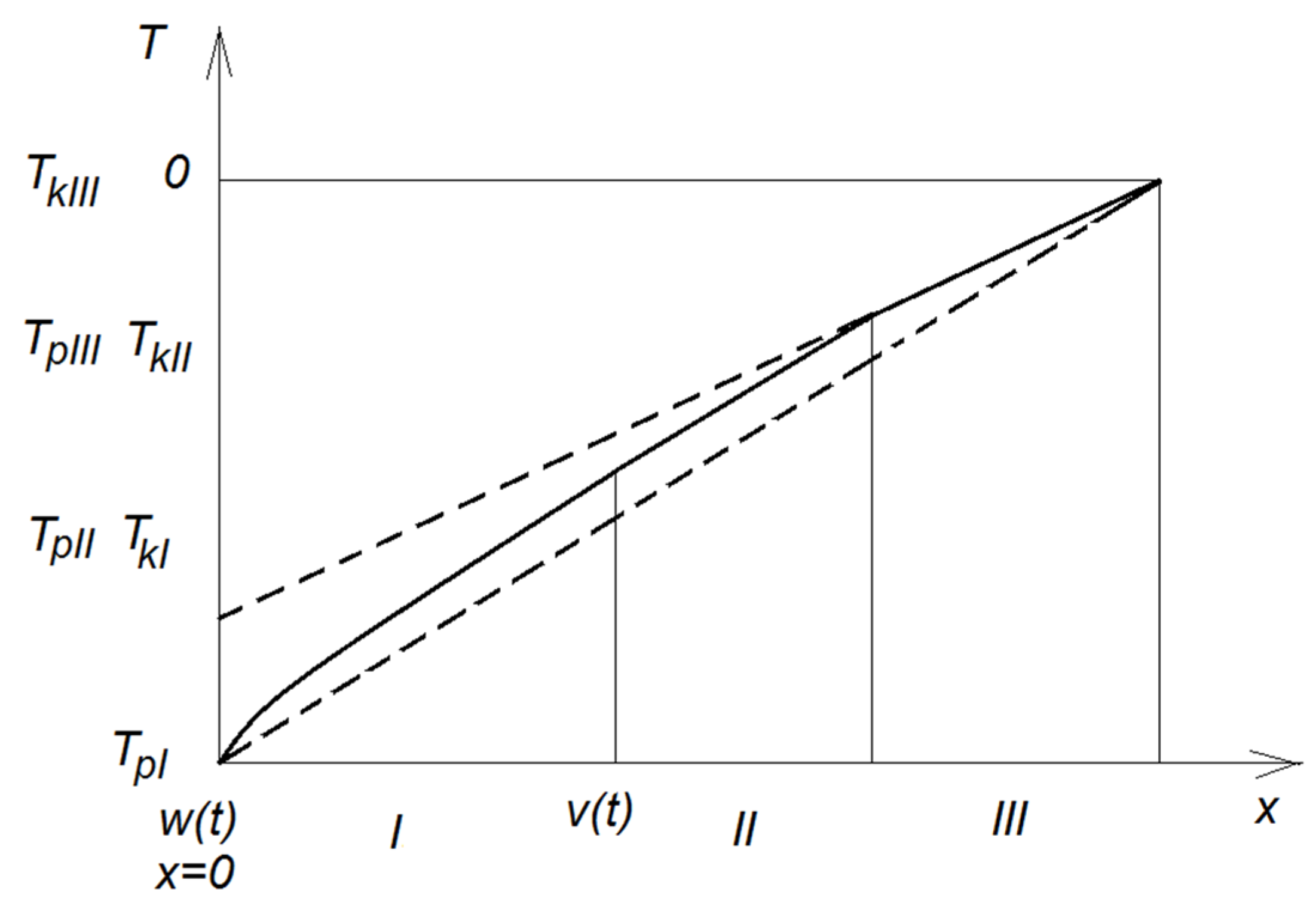
We assume that the beginning of the dynamic process is described by a function w ( t ) and end v ( t ) .
Temperature function on the section w ( t ) x < v ( t ) we assume in the form of
T w v ( t , x ) = a 0 ( t ) + a 1 ( t ) x + a 2 ( t ) x 2 + a 3 ( t ) x 3 .
In this section we will be integrating the Poisson equation.
On the domain v ( t ) x < g the function is linear with respect to x:
T v g ( t , x ) = A o ( t ) + A 1 ( t ) x ,
and satisfies the Laplace equation. 2 T ( x , t ) = 0 . General temperature distribution in the wall is shown on Figure 11.
Temperature function on the section w ( t ) x < v ( t ) we assume in the form of
T w v = a 0 ( t ) + a 1 ( t ) x ( t ) + a 2 ( t ) ( x ( t ) ) 2 + a 3 ( t ) ( x ( t ) ) 3 .
Dla x = 0 T = Δ T 0 p k + δ p r 0 a 0 = Δ T 0 p k + δ p r 0
Dla x = v(t) T k I = a 0 ( t ) + a 1 ( t ) x + a 2 ( t ) x 2 + a 3 ( t ) x 3
Dla x = w(t) T x = C 1     T x = a 1 ( t ) + 2 a 2 ( t ) x + 3 a 3 ( t ) x 2 a 1 ( t ) = C 1
From integrating the Poisson equation
T t = λ ρ c p Δ 2 T ( x , t ) .
Leibniz’s principle. Definite integral of derivative of function F(x,t) within w(t) to v(t) where w ( t ) x v ( t ) is equal to the derivative of the integral F(x,t) in the range from w(t) to v(t) minus the value of this function at the limits multiplied by the derivatives of the function “w(t), v(t)” in relation to time t. It can be called a change in the order of integration and differentiation.
T t = λ c ρ 2 T ( x ) .
By integrating the Poisson equation with the exploitation of the law of alternation of integration and differentiation, we obtained
d d t w ( t ) v ( t ) T ( x , t ) d x   T [ v ( t ) , t ] d v d t + T [ w ( t ) , t ] d w d t = λ c p [ T x x = v ( t ) T x x = w ( t ) ] .
t = D w ( t ) v ( t ) D T ( x , t ) d x = D w ( t ) v ( t ) T ( x , t ) d x   T [ v ( t ) , t ] d v d t + T [ w ( t ) , t ] d w d t
T(x, t) is the main causative function of the process changing from w(t) to v(t). We consider the diffusion of temperature T(x, t) resulting from a decrease in it on the left edge of a homogeneous belt of a flat medium. After the occurrence of a negative setpoint, the effect spreads to the entire considered zone of space, where the temperature function satisfies the Poisson equation.
d t w ( t ) v ( t ) T ( x , t ) T [ v ( t ) , t ] d v d t + T [ w ( t ) , t ] d w d t = λ ρ c p [ T x | x = v ( t ) T x | x = w ( t ) ] ,
d v d t = 0 ,   d w d t = 0 ,   T x | x = w ( t ) = C 1 , T x | x = v ( t ) = C 2 ,
w ( t ) v ( t ) T ( x , t ) d x = a o ( x ) x + 1 2 a 1 ( t ) x 2 + 1 3 a 2 ( t ) x 3 + 1 4 a 3 ( t ) x 4 | w ( t ) v ( t ) ,
w(t) = 0
w ( t ) v ( t ) T ( x , t ) d x = a o ( t ) v ( t ) + 1 2 a 1 ( t ) v ( t ) 2 + 1 3 a 2 ( t ) v ( t ) 3 + 1 4 a 3 ( t ) v ( t ) 4 ,
t w ( t ) v ( t ) T ( x , t ) d x = [ a o ( t ) v ( t ) + 1 2 a 1 ( t ) v ( t ) 2 + 1 3 a 2 ( t ) v ( t ) 3 + 1 4 a 3 ( t ) v ( t ) 4 ] v ( t ) t ,
Since v ( t ) t = 0
λ ρ c p [ T x | x = v ( t ) T x | x = w ( t ) ] = λ ρ c p [ C 2 C 1 ] = 0 C 2 = C 1 .
If the segment I is linear, the temperature function satisfies the Poisson integral equation.
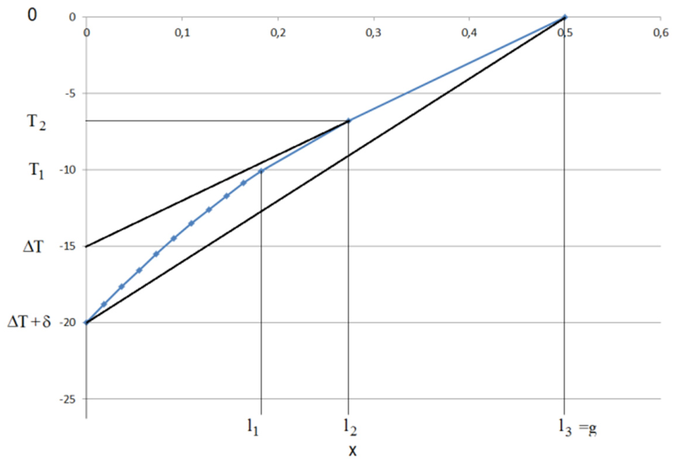
Hence, we can model processes that meet the Poison integral equation using linear functions as shown in Figure 9. In this case, the slope of the straight lines should be determined on three sections: I, II and III corresponding to the compliant ranges: the Poison integral equation, the ordered condition of Kondratieff and Laplace equation.
Range I
Temperature variability T l 1 = a 01 + a 11 x .
Boundary conditions
For x = 0 T = Δ T + δ a 01 = Δ T + δ .
The slope of the straight line l1 is denoted C1.
For x = 0 T x = C 1 a 11 = C 1 .
Based on [17] was adopted l 1 = 3.464 a t . The value of C1 can be written as
C 1 = T 1 Δ T δ l 1 .
Range II
Temperature variability T l 2 = a 02 + a 12 x
Boundary conditions
For x = l1 T = T 1 T 1 = a 02 + a 12 l 1 .
The slope of the straight line l2 is denoted C2
For x = l1 T x = C 2 a 12 = C 2
The slope of line l2 is assumed as the average of the slopes of straight lines C1 and C3:
C 2 = C 1 + C 3 2 .
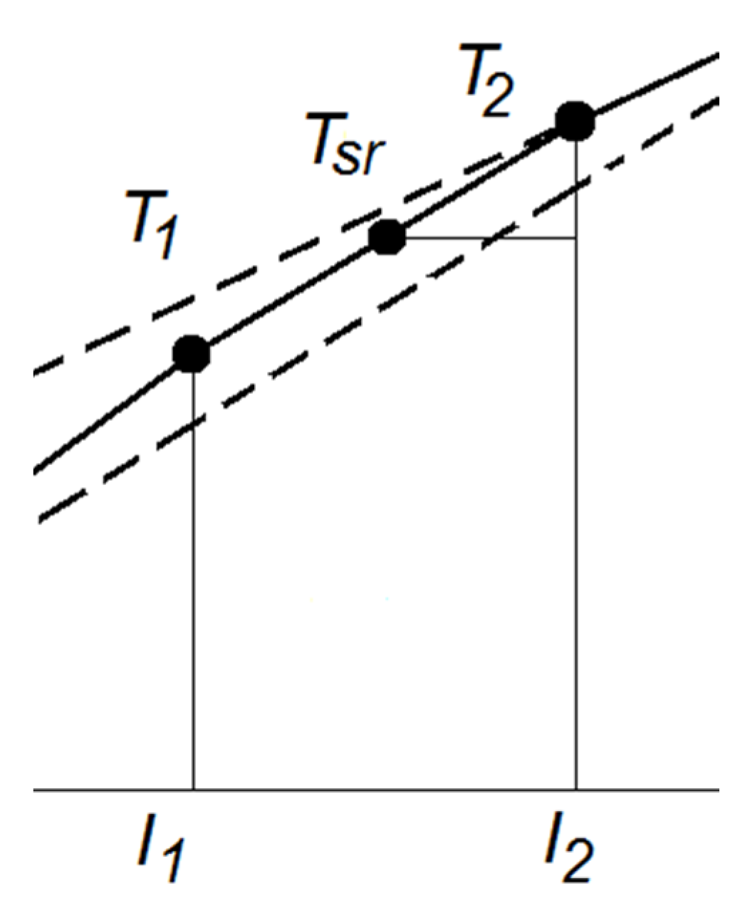
It was assumed that in the middle of segment l2 the temperature can be determined as the average of the calculations using the theory of ordered state as body cooling; it is marked by Tsr. The slope of the straight line can also be determined from the temperature Tsr and T2 as shown in the Figure 12.
C 2 = T s r T 2 0.5 ( l 2 l 1 ) .
Range III
Temperature variability T l 3 = a 03 + a 13 x
The slope of the straight line l3 is denoted C3.
For x = l3 = g, T = Tp, T p = a 03 + a 13 g .
For x = l2, T x = C 3 , a 13 = C 3 .
The straight line represents the initial steady state with a temperature difference ΔT. The slope C3 was calculated as
C 3 = Δ T g .

3.2.4. Example of Determining the Slope Coefficient of Straight Lines in Three Intervals

Let us determine the temperature distribution and straight slope coefficients for the selected time t = 10.000 s after the pulse appears.
l 2 = 3.464 a t .
We assume
l 1 = 2 3 l 2 .
Temperature T2
T 2 = Δ T g ( l 3 l 2 ) = Δ T g ( g 3.464 a t ) .
Temperature T1
T 1 = δ ( 1 x d ) 2 15 ( g x ) g .
Coefficient C1
C 1 = ( Δ T + δ ) T 1 l 1 = 54.3 .
Coefficient C2
C 2 = T 1 T 2 l 2 l 1 = 36.1 .
C3 factor steady-state slope
C 2 = T p T 2 g l 2 = 30 .
The calculated temperature distribution in subsequent stages of the process is shown in Figure 13.
Coeffcient C1 (97) is the inclination of the secant in segment l1.

4. Conclusions

The task of steady state analysis in a rectangular medium was presented and solved. The analysis of two cases of solutions with the different boundary conditions of the first kind is shown. These cases apply in the analysis of heat demand. In the standards, the calculation of heat demand was formulated as tasks of the steady state. In fact, the transition from one state to another must be resolved in transient assumptions. The article shows how to solve these three states. In the steady state example, there are continuous boundary conditions along the edge. Such tasks are useful in all aspects of building physics in rectangular areas. Additionally, the examples show how to decompose boundary tasks into four tasks based on symmetry features. In this way, we reduce the number of unknowns in the problem. The paper should not be viewed from the point of view of only needing to provide a numerical solution to specific tasks, but as an interpretation of the concepts and methods of solving detailed tasks in building physics, such as
  • Solution classes (polynomial solutions);
  • Breaking down the task into smaller ones with fewer constants (expressiveness of the task);
  • Forms of description of boundary tasks (number of conditions on the edges);
  • Simplicity of the form of solutions received.

Author Contributions

Conceptualization, S.O. and M.O.; methodology, S.O.; validation, M.O.; formal analysis, S.O.; investigation, S.O.; writing—original draft preparation, S.O.; writing—review and editing, M.O.; visualization, M.O.; supervision, S.O. All authors have read and agreed to the published version of the manuscript.

Funding

This research received no external funding.

Conflicts of Interest

The authors declare no conflict of interest.

References

  1. Balaras, C.A. The role of thermal mass on the cooling load of buildings: An overview of computational methods. Energy Build. 1996, 24, 1–10. [Google Scholar] [CrossRef]
  2. Levinskytė, A.; Bliūdžius, R.; Burlingis, A.; Makaveckas, T. Dependencies of heat transmittance through the ventilated wall system on thermal conductivity of connectors crossing thermal insulation layer. MATEC Web Conf. 2019, 282, 2089. [Google Scholar] [CrossRef]
  3. Medved, I.; Kalvoda, L.; Vejmelkova, E.; Vratislav, S.; Černy, R. Transport of gadolinium in a cement composite. MATEC Web Conf. 2019, 282, 2105. [Google Scholar] [CrossRef]
  4. Vlasov, V.Z. Method of initial functions in problems of the theory of elasticity. Bull. USSR Acad. Sci. 1955, 7, 49–69. (In Russian) [Google Scholar]
  5. Lur’e, A.I. Three Dimensional Problems of the Theory of Elasticity; Gostehizdat: Moscow, Russia, 1955. (In Russian) [Google Scholar]
  6. Owczarek, S. Wielomianowa Postać Rozwiązania Zagadnień Statyki Sprężystych Tarcz Prostokątnych; IFTR Reports nr 17; Institute of Fundamnetal Technological Research PAS: Warsaw, Poland, 1984. (In Polish) [Google Scholar]
  7. Patel, R.; Dubey, S.K.; Pathak, K.K. Infilled reinforced concrete beams for sustainable construction. J. Civ. Eng. Archit. 2013, 7. [Google Scholar] [CrossRef] [Green Version]
  8. Patel, R.; Dubey, S.K.; Pathak, K.K. Analysis of RC brick filled composite beams using MIF. Procedia Eng. 2013, 51. [Google Scholar] [CrossRef] [Green Version]
  9. Aste, N.; Angelotti, A.; Buzzetti, M. The influence of the external walls thermal inertia on the energy performance of well insulated buildings. Energy Build. 2009, 41, 1181–1187. [Google Scholar] [CrossRef]
  10. International Organization for Standardization (ISO). Thermal Performance of Buildings–Transmission and Ventilation Heat Transfer Coefficients—Calculation Method; ISO 13789; International Organization for Standardization (ISO): Geneva, Switzerland, 2017. [Google Scholar]
  11. International Organization for Standardization (ISO). Thermal Performance of Building Components—Dynamic Thermal Characteristics—Calculation Methods; ISO 13786; International Organization for Standardization (ISO): Geneva, Switzerland, 2017. [Google Scholar]
  12. Ma, P.; Wang, L.-S. Effective heat capacity of interior planar thermal mass (iPTM) subject to periodic heating and cooling. Energy Build. 2012, 47, 44–52. [Google Scholar] [CrossRef]
  13. Kossecka, E.; Kosny, J. Influence of insulation configuration on heating and cooling loads in a continuously used building. Energy Build. 2002, 34, 321–331. [Google Scholar] [CrossRef]
  14. Collet, F.; Serres, L.; Miriel, J.; Bart, M. Study of thermal behaviour of clay wall facing south. Build. Environ. 2006, 41, 307–315. [Google Scholar] [CrossRef]
  15. Stazi, F.; Tomassoni, F.; Veglio, A.; Di Perna, C. Experimental evaluation of ventilated walls with an external clay cladding. Renew. Energy 2011, 36, 3373–3385. [Google Scholar] [CrossRef]
  16. Pogorzelski, J.A. Fizyka Cieplna Budowli; Polish Scientific Publishers (PWN): Warsaw, Poland, 1976. (In Polish) [Google Scholar]
  17. Taler, J.; Duda, P. Rozwiązywanie Prostych i Odwrotnych Zagadanień Przewidzenia Ciepła; Wydawnictwa Naukowo-Techniczne (WNT): Warsaw, Poland, 2003. (In Polish) [Google Scholar]
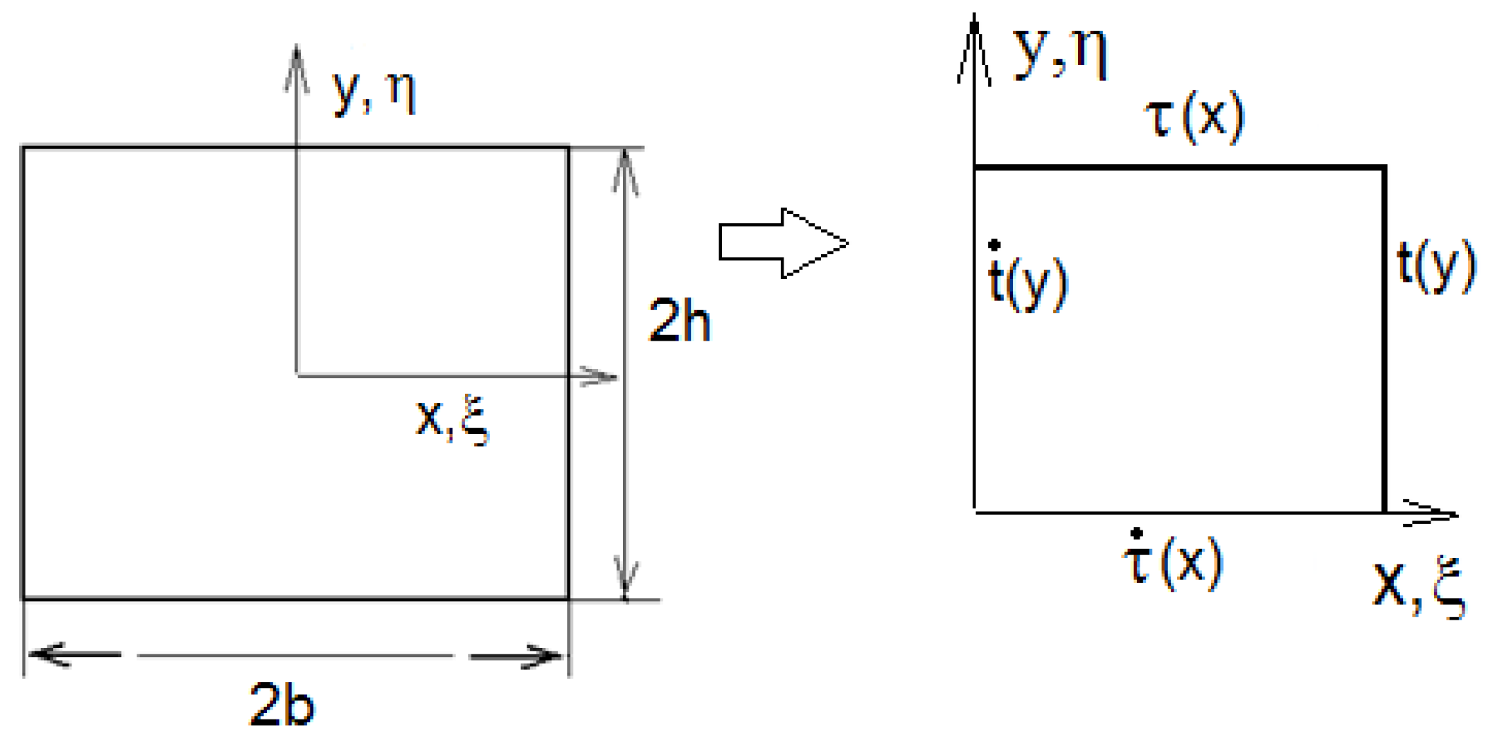
Figure 1. Coordinate system adopted in the analysis.
Energies 13 01714 g001
Figure 2. Dimensions of the analyzed building partition.
Energies 13 01714 g002
Figure 3. Example of boundary conditions of temperature in the shield.
Energies 13 01714 g003
Figure 4. The symmetrical part of the task. SS state.
Energies 13 01714 g004
Figure 5. Antisymmetric part relative to x and symmetric to y. AS state.
Energies 13 01714 g005
Figure 6. Temperature map calculated in Example. The dimensions of sides h/b = 6.
Energies 13 01714 g006
Figure 7. Steady-state temperature on the edges of Plate 2.
Energies 13 01714 g007
Figure 8. Image of temperature in the shield in State 2.
Energies 13 01714 g008
Figure 9. Geometry parameters and boundary conditions of the formulated problem.
Energies 13 01714 g009
Figure 10. Graph of the temperature after the dynamic effect has occurred.
Energies 13 01714 g010
Figure 11. Temperature function on the sections w ( t ) x < v ( t ) and v ( t ) x < g caused by an impulse.
Energies 13 01714 g011
Figure 12. Principle of determining the slope coefficient of the C2 range.
Energies 13 01714 g012
Figure 13. Calculated temperature distribution.
Energies 13 01714 g013
Table 1. Divalent and trivalent functions used in Equations (35)–(38).
n0123456
j(n)1010101
J(n)10−1010−1
j(n + 1)0101010
J(n + 1)0−1010−10