1. Introduction
The trend of the last decade to reduce greenhouse gas emissions and decarbonize the energy sources is mainly due to the increase of the temperature of the planet, has driven the development and improvement of technologies for renewable energy sources. As well known, solar energy is the most available renewable energy source in the world with respect to the other sources and an interesting topic of research is the evaluation of its economic convenience. For this reason, in many studies reported in literature, the economic convenience of grid-connected PV systems has been evaluated with respect to other technologies. The traditional approach is based on the use of the “levelized cost” method that represents the per unit value of total costs (i.e., capital, operation and maintenance, fuel) over the economic life of the power plant [
1,
2]. The notion of economic convenience of PV plants emerged from these studies.
In the European Union (EU), the number of the PV plants is increasing significantly thanks to the policies of the different countries that have led to economic benefits for private citizens and in particular for small size PV plants called “residential plants” (from 1 kWp to 10 kWp) through diverse incentive systems. The international policies to encourage the installation of the PV plants usually consist of an incentive for the total “green energy” produced and in an incentive for the energy injected into the grid only for the grid-connected plants.
As well known, a typical issue of PV plants is the power loss due to the differences of irradiation (partial shading or wrong design) among the cells of the same module or among different modules of an array. This phenomenon, known as mismatch, can generate a considerable power loss of the total system with a consequent economic loss. In [
3] an interesting estimation of PV mismatch losses caused by moving clouds is reported. Moreover, this phenomenon can be caused from a fixed obstacle that may have appeared years after the installation of the PV plant. The presence of a fixed obstacle after the installation is a frequent case in residential PV plants.
In order to limit the mismatch phenomenon, monitoring systems are extensively used in renewable energy applications to track the performance of the generation plant. A monitoring system for PV arrays is usually needed to collect power production and performance data as well as weather condition information and relate them [
4,
5,
6]. These systems allow detecting fault conditions, but they are not effective for estimating the power reduction of a PV plant.
The issue of the different irradiation levels among the cells of a module has been studied in [
7], where an investigation on partially shaded modules with different PV cell connections was reported. The authors compared five different connection configurations in order to find the best solution to increase the maximum power production and the fill factor of a module. The same problem has been studied in [
8] and [
9].
The different irradiance causes also problems in maximum power point tracking (MPPT) algorithms because the P-V curves of the PV module exhibit multiple maximum power points due to the bypass diodes, which are used to exclude the module of an array. In [
10], the authors classified MPPT techniques for different PV array configurations. Obviously, each method presents advantages and drawbacks. Again, an interesting MPPT strategy for PV arrays under uniform and non-uniform irradiance condition is described in [
11].
A recent solution proposed in the literature to reduce the power losses is the use of a dynamic reconfiguration system (DRS). The DRS allows one to change the configuration of the PV plant in order to increase the power production. Different solutions have been recently proposed in literature to optimize the power output adopting dynamic reconfiguration systems for PV module interconnection [
12,
13,
14,
15,
16,
17,
18,
19].
An interesting topic about DRS concerns the economic benefits introduced by the use of these systems. In [
20] a technical-economical evaluation on the use of a DRS in some EU countries for PV plants is reported. In particular, by considering the incentive policies and others technical aspects of a 3 kW PV plant the NPV have been evaluated for each country taken into account. Nevertheless, in this study the technical aspects and different configurations of the DRS were not considered. For this reason, it is necessary to extend the economic analysis by introducing the real technical considerations of the DRS for different configurations reported in literature.
The aim of this paper is to evaluate the economic benefits accrued by using a DRS in a residential PV plant. First, an economic analysis of different DRSs according to the costs of the components and to the adopted topological schemes, is carried out; to the authors’ knowledge, this issue has never been addressed in the technical literature. Architectures involve switching matrix, sensing network and driving circuit, the choice of switches affects the electro-technical and, electrical endurance. As will be shown in the following sections, the choice of a more flexible DRS comprises higher initial cost due to the number of switches required by the adopted architecture, but at the same time a less exploitation and therefore a longer useful life.
In particular, the study takes into account different technical and economic aspects of a PV plant in order to present a complete economic analysis. In other words, the study is focused on the use of different DRS configurations reported in literature, in some EU countries in order to evaluate the performances of the investment. The economic tools are the net present value (NPV) and payback time.
This paper is organized as follows:
Section 2 provides a brief description of the DRS topology taken into account in this work and technical considerations to estimate the costs and lifetime of DRS.
Section 3 describes the experimental set-up to perform the evaluation of performance of DRSs. In
Section 4 the economic data are reported and in
Section 5 the economic results are presented. Finally,
Section 6 concludes the paper.
2. Dynamic Reconfiguration Systems
A DRS allows changing the connections among PV modules in order to increase the total power production from a PV plant under poor irradiance conditions or other situations, that determine the degradation of the performance. In this way, the hardware complexity of the DRS depends on the possible connections among the modules. Generally, in a reconfiguration algorithm each panel is a considered a node of the dynamic array; the number of the nodes is identified as m while n switches perform the dynamic connections among the panels. A plant with a high number of panels requires a DRS with a high number of switches in order to connect all the nodes. Thus, a topology with more switches guarantees a high number of possible configurations for connection of the panels. In this section, a brief state of art of the dynamic reconfiguration systems (DRS) and a technical-economic analysis of the four cases studied, are reported.
2.1. Case Studies
In order to carried out a complete technical-economic analysis, four DRS cases have been investigated. The same cases have been studied in [
21], but without considering the implications in terms of cost and lifetime of the DRS. The first case under test has been presented in [
22]. The authors proposed an optimised switch set (SWS) topology for reconfiguration of PV panels based on a particle swarm optimization (PSO) algorithm.
Figure 1 shows the optimised topology structure suggested by the authors, in which there are four lines and ten switches.
From
Figure 1, it is possible to observe that the number of switches
n for each node
m, is equal to:
An interesting low-cost method has been presented in [
23]. This method does not require any additional MPPT controllers or sensors and it is based on the use of fuzzy logic (FL) which is used to identify shaded, dirty or faulty panels, to estimate the percentage of shading or dust and to evaluate the minimum and maximum voltage values at which PV panels should be connected/disconnected. The validity of this system has been demonstrated through experimental tests.
Figure 2 shows the connection of the system with four panels described in case 2.
The number of switches required for the case 2 can be evaluated as:
In [
24] a photovoltaic array switching algorithm is presented. This algorithm, in order to find the best configuration of a PV array, is based on the use of only two parameters: the array load voltage and the PV module’s temperature. The study has been focused on the evaluation of the performance of four PV modules, as shown in
Figure 3.
The number of switches necessary in case 3 is equal to:
The last case taken into account in this work is presented in [
25]. Case 4 is a system configuration approach using an adaptive architecture based on a switching matrix. The adaptive strategy is based on the fact that the switching matrix allows one to rearrange the active PV modules in series into multiple strings to meet the required voltage level.
Figure 4 shows the proposed switching matrix of case 4.
Also, in this case, the number of switches of the matrix depends by the number of modules in the PV array. The number of switches can be expressed as:
where the terms 2
dc and 2
inv represent the switches to connect the PV array with the inverter and the direct current converter. In the next section, the cost estimation analysis is reported.
2.2. Costs Estimation of DRS
The cost of each reconfigurator system has been evaluated on the basis of the direct proportionality between the number of switches composing the system and the cost of the technology needed to produce it.
For each of the four considered reconfiguration cases, a cost estimation of the reconfiguration system has been carried out according to the following procedure: for each case, the required amount of components has been evaluated; after that, for each type of electrical component, a specific item which is available on the market has been chosen, compliant with the technical requirements of the system; finally, for each of the selected components, a price is given, as provided by a major distributor of electronics [
26].
Generally, the hardware of a dynamic reconfigurator basically consists of three different parts: the switching matrix, the sensing network and the driving circuit. The switching matrix includes all the switches that are used in the reconfiguration system. Taking into account the solutions available in the market, each switch is generally assembled through two parallel-connected devices: an electromechanical relay and a semiconductor device, e.g., a MOSFET [
27,
28]. A state-solid relay is a valid alternative as well, but it turns out to be more expensive. Whenever the switch has to be put in the off state, the semiconductor switch is closed as first, so that the electromechanical switch can be switched off at a low voltage. When the switch is on, the electromechanical relay guarantees the conduction losses minimization. In this way, the current breaking capability of the electromechanical switch is fully employed, since it is better to be opened at a quite low voltage. The number of parallel-connected MOSFETs arises from the type of electromechanical switches: one MOSFET has to be connected to one single pole single throw (SPST), whereas two MOSFETs have to be connected to one single pole double throw (SPDT). In
Table 1 the chosen electromechanical relays are reported along with their respective prices [
26,
29,
30].
In
Table 2 the selected MOSFETs and drivers and respective prices are reported as well [
26,
31,
32].
As far as the sensing network, three types of measurements are generally needed: voltage, current and temperature. In all four cases provided in this paper no irradiance sensor is required. The electronics involved in the voltage sensing circuit are normally very cheap, therefore voltage sensors are not considered in the hardware balance for the sake of simplicity. The selected sensors of temperature and current and their price are reported in
Table 3. Note that for the current measurement, the selected sensors are compliant with a 6A rated current [
26,
33,
34].
Table 4 provides the details concerning the number of the different components which should be used in the four considered reconfiguration cases: PV modules (Np), SPST and SPDT switches (N
SPST and N
SPDT), MOSFETs, drivers and sensors. The total price has been calculated according to the cost tables previously reported.
2.3. Lifetime Estimation of DRS
The lifetime of each reconfiguration solution has a significant contribution to the overall economical impact, even though in the scientific literature this aspect is generally neglected [
35] Regarding this, the most important issue to be addressed is the lifetime of the relays, due to their mechanical characteristics. Both the electrical and the mechanical endurance are reported in the technical datasheets. Indeed, both the electrical and the mechanical behaviour of the relay are affected by the switching operations. More in detail, the electrical endurance, given by the maximum number of cycles recommended to not affect the electrical behaviour of the relay, is usually much shorter than the maximum number of cycles recommended not to affect the mechanical behaviour. Therefore, being first in the time course, only the electrical endurance has been considered in the overall lifetime estimation.
As reported in the technical datasheets, the maximum number of cycles for the selected SPST switches is 10
5, whereas for the selected SPDT switches this value is 60 × 10
3 [
29,
30]. In order to evaluate the actual number of switching operations for each reconfiguration case, the specific algorithm as well as the irradiance conditions should be exactly known. Nevertheless, being these data due to the designer in the first case and unpredictable in the second, a simple approach has been here adopted. Considering N
SPST and N
SPDT the number of SPST and of SPDT respectively, the probability of a switching operation for each of them has been considered to be 1/N
SPST and 1/N
SPDT. These are meant to be the probability values whenever the algorithm and the irradiance condition lead to a reconfiguration operation. As far as the hours of sunlight and the frequency of reconfiguration are concerned, two “worst case” values have been considered: 16 h of sunlight and 1 reconfiguration every minute. Even though these values are generally peak values across the whole day, these are meant to be the average values, so that a “worst case” situation is taken into account. In
Table 5, the number of considered sunlight hours, the number of considered reconfiguration operations per minute and the electrical endurance of SPST and SPDT are given, referenced as E
SPST and E
SPDT, respectively.
According to the 16 light hours and one reconfiguration per minute, 350,400 operations are calculated per year, so that the corresponding number of reconfiguration per switch is calculated, according to (5):
where:
Ryr is the number of reconfigurations per year;
Ryrsw,SPST and
Ryrsw,SPDT are the number of reconfigurations per year per switch for SPST and SPDT respectively;
Nyr,SPST and
Nyr,SPDT express, in terms of number of years, the endurance of SPTS and SPDT switches respectively.
Table 6 reports the data referring to both types of switches and to the four considered cases of reconfiguration, obtained from (5). Note that the number of total reconfigurations
Ryr has been considered the same for all the cases.
According to that, the total cost evaluation, including the overall system, is considered and reported in
Table 7 for different cases of years to come before the switches are changed.
The economical contributions concerning the switches and the overall system, as reported in
Table 7, arise from the data reported in
Table 1 and
Table 2, respectively. Note that the configurations with the lowest number of switches are less convenient if only the price of the switches is considered, supposing that in the same number of years they require to be changed a higher number of times. On the contrary, if the total cost of the reconfigurator is considered, the cases with the lowest number of switches are the most convenient. Indeed, the initial price in terms of sensors, drivers and MOSFETs is generally higher if the number of mechanical switches is higher, due to the higher hardware complexity. Note as well as that if a low number of switches is associated to a more complex algorithm, so that the reconfiguration frequency is higher, the frequency of maintenance increases. As an example,
Table 8 refers to two reconfigurations per minute in case 2, whereas the number of reconfigurations per minute in the other cases is kept at 1.
One can see that in this case the most convenient solution, after 30 years, is the one corresponding to the case 3. Although the obtained economical results of this comparison among different reconfiguration cases shall not be critically considered, what is significant in this paragraph is the proposed approach for an economical estimation of the system lifetime.
3. Experimental Set-Up
Figure 5 sketches a realistic situation in which, during the day, a shadow overlays different panels. As a consequence, the shadowed panels disturb those connected in parallel: a decrease in voltage of shadowed panel involves a decrease of not shadowed ones and a rise of current for the power balance. This rise of current is not constantly probable: if the not shadowed panels are in the area of maximum power point, any decrease of voltage decreases the power.
Figure 6 shows the effect of a shadow due to the presence of a pole by considering a PV DRS scheme. The hypothesis is that each panel has three lines of cells and is connected to the DRS. DRS is connected to a two channels inverter.
Reconfiguration performances were tested with a prototype DRS developed at the University of Palermo and working on a twelve panels system. DRS acquires the state of every panel with a sensing system (voltage, current and temperature).
Figure 7 shows the experimental DRS system. Twelve panels (PMMP 215 W, VMPP 28.27 V, IMPP 7.59 A, Voc 36.37, Isc 8.21 A, Conergy, (Hamburg, Germany) have been connected individually to the DRS. Panels located at latitude: 38° 5.9’; longitude: 13° 20.6’, measurement carried out in the morning of 27 April 2016, from 10:00 to 13:00, with incident radiation between 1.0 and 1.1 kW / m
2 and temperature between 20–25 °C.
Without shadows, each panel works in the same point: the DRS generates basic topology, in this case, two parallel identical strings of six modules in series. To perform the behavior of the DRS, different resistive loads have been considered and
Table 9 lists the different working conditions.
In order to test the DRS, an artificial shadow has been created.
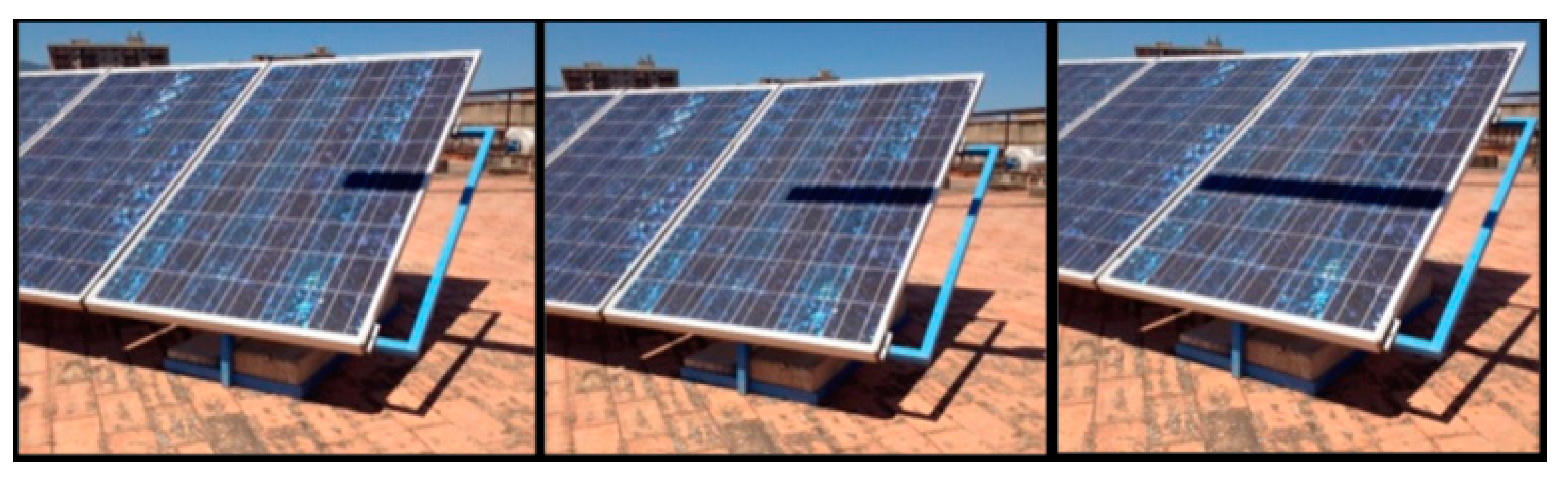
Figure 8 displays three shadow cases for a panel connected in series with five others. The artificial shadow cuts one, two or three lines of modules, dropping the performance of the panel and of the string. Each stoppage of line requires the action of the bypass diode, and a successive voltage decrease of the panel. The shadowed panel has labelled with the number 6, so V1–V5 are the voltages of normally irradiated panels and V6 is the shadowed one; DRS evaluates the power of each panel and connects the panels into the string.
Table 10 recapitulates the behavior of the DRS with shading and without; P
1–P
5 are the powers of the not shadowed panels, P
6 is the power of the shadowed one in three cases, I is the current of the system in the different cases taken into account
Figure 9 and
Figure 10 show respectively the voltage-current and voltage-power profiles of the panel with three working lines of cells, two working lines of cells and only one working line. Blue curves describe the working points without any shading. If a line of cells is shaded the orange curve has to be considered, maintaining a similar current and with a new voltage. When a shadow covers two lines of cells from the blue curve the gray curve has to be considered, maintaining a similar current and with a new voltage.
New voltages indicate the new power conditions. The DRS is able to regroup similar irradiated panels and/or exclude the densely shaded panels. The different operation is due to the DRS architecture and the algorithm implemented. A not smart DRS can only exclude shaded panels, a high-performance DRS relocates them on suitable dynamic arrays.
3.1. Evaluation of Power Losses for a Single Shaded Panel
In the following part three cases are evaluated: case 1, only a line has been interrupted; case 2, two lines were interrupted; case 3, the whole panel is shadowed. By excluding the shaded panels there will be 16.7% of losses. DRS can enable the power increases shown in
Table 11.
Data presented in
Table 11 can be plotted in
Figure 11: in case 1 and for the lower currents (load A, B and C) there is an increase of power, for higher currents (loads D and E) there is a decrease; in case 2, for lower currents (loads A, B, C and D) there is an increase, for the higher current (load E) there is a decrease.
Case 3 is now considered: the shadow cuts entirely the panel, as shown in
Figure 8. A negative voltage of the shadowed panel affects the performance of the string. Each not shaded panel varies its operating condition assuming a voltage slightly higher than the non-perturbed, to compensate the voltage drop on the shaded panel and to try to maintain a high current.
Table 12 shows the increase of power when a panel is totally shaded. The study of case 3 shows that when the shadows cuts in two parts the panel 6 and it becomes a load, reconfiguration reduces always the loss of power.
Case 3 shows the real performance of the DRS. Between loads C and D the maximum power point is performed. By considering the overall behavior of two shaded strings used simultaneously, a possible performance increase between 12 and 25% can be expected.
3.2. Evaluation of Power Losses for two shaded panels
The previously obtained performances only consider a shaded panel, and the logic is to maintain it (partially shaded) or exclude it (totally obscured). Now if two panels are shaded there is the possibility of placing in parallel. Panels named 6 and 7, can be re-configured to ensure the maximum current of the arrays. This feature requires a more evolved DRS, which can put in parallel panels belonging to different arrays, the sum of which currents is equal to the current of not obscured panels. This feature is useful only when it considers case 2 as shown in
Table 13. The performances of different DRS are a mixture of the ones presented in
Table 12 and
Table 13. For the economic analysis the increased power given by the reconfigurator is taken as an increase of the energy produced during the day.
4. Economic Data
In order to carry out a complete study, the economic analysis presented in this paper takes into account different aspects of a PV plant, such as PV technology, location of the installation, government incentives, component lifetime, aging and periodic maintenance costs.
This study is based on the use of economic a tool called net present value (NPV), in order to evaluate the benefits of an economic investment in PV field with innovative devices such as a DRS. The NPV allows to evaluate the economic convenience of an investment for a specific period from a sum of cash flows actualized at time zero. In (6) the mathematic expression to evaluate the NPV is reported:
With reference to expression (6), C0 is the cash flow at time zero, Cy is the cash flow at the year y, i is the interest rate and y is the year of investment. Thus, the sign of the NPV, positive or negative, indicates the infeasibility of the investment and therefore the economic convenience. The interest rate i% considered in this work is equal to 5%. In this study, the technical-economic analysis has been carried out by considering an investment time equal to 20 years. In the following, detailed description of different aspects taken into account for the economic analysis and economic data are reported.
4.1. PV Plant
Since the first PV plants became commercially available on the market the cost of PV components, installation and maintenance has changed notably. In particular, in the last years there has been a constant decrease of the costs on the world market.
In this study, only residential PV systems with 6 kWp of power have been taken into account. This choice is motivated by the fact that the use of DRS is very interesting in residential PV plants, where the probability of installation of a fixed obstacle is high in respect to other type of plants. Indeed, four years after the installation, a fixed obstacle reducing by 35% the total power is assumed to appear. This value of reduction has been demonstrated in study [
20]. Moreover, in order to carry out a complete analysis among different locations of installation taken into account, an installation of the PV plant between 2013 and 2014 was assumed, considering that in those years there were incentives in all the countries.
Regarding the cost of the PV plant, the average estimated price for this type of plant is about 2500 €/kWp (included installation). In
Table 14 the economic data about the PV plant under test are summarized.
4.2. Location of Installation and Economic Aspects
The installation location represents an interesting point of analysis in terms of production capability, government incentives and payments to private citizens for the production of the energy. Moreover, also the lifestyle of people plays an important role and therefore the average consumption per capita of the electric energy. In order to extend the economic analysis Italy, Germany, France, Spain, Bulgaria, Romania, Greece and Croatia have been considered as reference countries. As well known, these countries have different PV plant performances, different policies to improve the use of electricity generated from renewable sources and different people’s lifestyle. In detail, the common strategy is based on a feed-in tariff (FIT) system with different values and timing of the incentives.
The economic data for each country (average consumption per capita, production facility, energy cost and incentives) have been referred of a PV plant installed in the capital of each countries. Moreover, has been considered a family composed by four people that lives in the capital of each countries. In
Table 15 the considered economic data are reported.
These data are based on the following consideration:
a family composed of four members and living in each capital of the considered countries;
the electrical energy produced per year by a 6 kWp PV plant has been taken into account.
the installation of the plant has been assumed between the year 2013 and 2014.
It should be noted that France has the highest value of average consumption per capita. This data is very high with respect to the production facility of the PV plant, so the analysis for the use of DRS is particularly difficult. The higher value of the energy production is in Greece, whereas, Romania and Croatia only offer incentives for 15 and 12 years. It should be noted that these considerations have influenced the economic results.
4.3. Inverter
The inverter represents the heart of the production from the solar energy. In particular, as well known, this system allows the electric energy conversion from DC to AC in order to inject the power surplus into the grid. Therefore, in the case of inverter fault it is not possible to use the energy with a consequence economic loss. From different studies, it is known that the inverter is the component more sensitive to failure. In [
2], the authors considered an inverter life equal to 10 years. Nevertheless, it is not possible to estimate with accuracy the lifetime of an electronic component. For this reason, by considering a possible worst case, in this study it was assumed that the average lifetime of the inverter is equal to seven years. As far as the cost is concerned, according to [
36] for a residential PV plant with 6 kWp of power the average cost is equal to 1000 €.
4.4. Increase of Production by DRS
The purpose of a DRS system is to increase the power of a PV plant in the case of a reduction of the total power production. The increment of the power production is a parameter that depends on the DRS topology and therefore hard to estimate. Indeed, the increment of power depends on the type of DRS and therefore of the number of possible available configuration. Thus, the number of possible reconfiguration available play an important role. By considering that a DRS with high number of switches allows many reconfigurations with respect to a DRS with a low number of switches, it is supposed to provide a higher increment of power. Nevertheless, this consideration is not enough to estimate the increment of power provided by a DRS with a defined number of switches, because it is possible that a DRS with high number of switches has redundant configurations. For this reason, in this work the same value of power increment has been considered for each DRS and fixed equal to 10% for the sake of simplicity. This obviously represents an unfavourable condition for DRS with high number of switches and higher costs. Nevertheless, this choice allows to emphasize the effect on the economic analysis of the costs and lifetime for each DRS.
4.5. Aging and Maintenance of PV Plant
After the installation, a natural phenomenon is the aging of the PV components. This phenomenon causes a reduction of the power and it increases over the time. Thus, in the economic analysis has been considered a reduction of power after the first year of the installation equal to 3% and a reduction for each year equal to 0.5%. Moreover, also a periodic maintenance has been considered with a cost equal to 100 €/year.
5. Economic Results and Discussion
As described above, the economic analysis of this study is focused on the evaluation of the economic benefits by using a DRS system four years after the installation of the PV plant with a power reduction equal to 35%. In particular, four cases of DRS have been analysed in different EU countries in order to extend the economic results.
Figure 12 shows the NPV trend over the time of four cases of DRS
1-4 and without DRS for each country.
The best result has been obtained in Spain with the highest value of the NPV after 20 years due to the incentives per year. Positive NPV values have been obtained in Italy, Bulgaria and Greece thanks to the high values of the production facility. Romania and Croatia have been penalized for a lower duration of the incentives, whereas, France and Germany have been penalized for the lower values of the production facility. The values of the NPV for each country and for each DRS are summarized in
Table 16.
By analysing the NPV values of
Table 16, it is interesting to note that DRS
4 allows one to obtain the best results also in the cases in which there the negative values of NPV. Moreover, this result is interesting because the DRS
4 present the second highest cost equal to 1148 € also by considering the worst case for the DRS with higher costs. Other interesting consideration can be done by changing the increment power. By considering an increment of the power equal to 20%, the NPV values obtained are reported in
Table 17.
In respect to the previous case, the DRS
4 with an increment of power equal to 20% allows to obtain positive values of the NPV also for Romania and Croatia. This result is realistic because the DRS
4, thanks to the high number of switches and thus the high number of the possible configurations, may generate an increment of power equal to 20%. Another interesting point of analysis is the payback time. In
Table 18, the payback times for each country and for each DRS in two power increment cases are reported.
Spain and Italy present the best results and it is interesting to note that the same values in the two cases of the increment of power have been obtained. In other countries (Germany, France and Romania), it was necessary to extend the duration of the investment in order to find the payback time but in all cases the best results have been obtained with DRS4 and an increment of power equal to 20%. Only in Bulgaria and Greece a reduction of the payback time has been obtained, an increment power equal to 20%, 13 years to 12 years and from 15 years to 12 years, respectively.
6. Conclusions
This paper presents a complete analysis on the real benefits introduced by a DRS system in a PV plant after a considerable power reduction. In particular, in order to evaluate the overall economic impact on the costs of a PV plant the technical and economic aspects about the DRS have been considered. In the first part of the paper an economic analysis of different DRSs due to the costs of the components and to the adopted topological schemes, is carried out. Switching matrix, sensing network and driving circuit constitute the architecture of DRS, the choice of switches and their number affects the electrical endurance. A more flexible DRS involves higher initial cost due to the number of switches required by the adopted architecture, but at the same time a less exploitation and therefore a longer useful life.
From the economic point of view, the analysis has been extended to different countries of EU in order to considerate incentives policies, location of installation and lifestyles of the people, while, from a technical study, that takes into account the hardware complexity in terms of the components required and other technical aspects, the costs and lifetime of four DRS have been estimated. The economic tool used in this analysis is the NPV and the payback time.
Firstly, in all scenarios the analysis has demonstrated the positive economic impact on the use of a DRS in a PV plant with respect to the cases without DRS. The best results have been obtained in Spain thanks to the higher value of the incentives per year in terms of NPV and payback time, whereas good results have been obtained for Italy, Bulgaria and Greece. The worst results have been obtained for France and Germany due to the lower values of the production facility. Among the DRS considered in the economic analysis, the DRS4 option allows one to obtain the best results in all cases. The best performance of DRS4 is attributable to the high number of switches that allows it to increase the lifetime of the system.
Author Contributions
Conceptualization, F.V.; methodology, F.V. and P.R.; software, G.S. and F.P.; validation, F.P. and G.S.; formal analysis, F.V. and G.S.; investigation, P.R. and F.V.; resources, R.M. and G.A.; data curation, G.S. and F.P.; writing—original draft preparation, F.P., G.S., and F.V.; writing—review and editing, G.A. and F.V.; visualization, G.A. and R.M.; supervision, G.A., R.M. and F.V. All authors have read and agreed to the published version of the manuscript.
Funding
This research received no external funding. This work was financially supported by MIUR-Ministero dell’Istruzione, dell’Università e della Ricerca (Italian Ministry of Education, University and Research) and by SDESLab (Sustainable Development and Energy Saving Laboratory) and LEAP (Laboratory of Electrical APplications) of the University of Palermo.
Conflicts of Interest
The authors declare no conflict of interest.
References
- Timilsina, G.R.; Kurdgelashvili, L.; Narbel, P.A. Solar energy: Markets, economics and policies. Renew. Sustain. Energy Rev. 2012, 16, 449–465. [Google Scholar] [CrossRef]
- Branker, K.; Pathak, M.J.M.; Pearce, J.M. A review of solar photovoltaic levelized cost of electricity. Renew. Sustain. Energy Rev. 2011, 15, 4470–4482. [Google Scholar] [CrossRef] [Green Version]
- Lappalainen, K.; Valkealahti, S. Photovoltaic mismatch losses caused by moving clouds. Sol. Energy 2017, 158, 455–461. [Google Scholar] [CrossRef]
- Zou, X.; Li, B.; Zhai, Y.; Liu, H. Performance monitoring and test system for GridConnected photovoltaic systems. In Proceedings of the 2012 Asia-Pacific Power and Energy Engineering Conference, Shanghai, China, 27–29 March 2012. [Google Scholar]
- Caruso, M.; Miceli, R.; Romano, P.; Schettino, G.; Spataro, C.; Viola, F. A low cost, Real-time monitoring system for PV plants based on ATmega 328P-PU Microcontroller. In Proceedings of the 2015 IEEE International Telecommunications Energy Conference (INTELEC), Osaka, Japan, 18–22 October 2015. [Google Scholar]
- Caruso, M.; Di Tommaso, A.O.; Miceli, R.; Ricco Galluzzo, G.; Romano, P.; Schettino, G.; Viola, F. Design and experimental characterization of a low cost, real-time, wireless, AC monitoring system based on ATmega 328P-PU microcontroller. In Proceedings of the 2015 AEIT International Annual Conference (AEIT), Naples, Italy, 14–16 October 2015; pp. 1–6. [Google Scholar]
- Wang, Y.-J.; Hsu, P.-C. An investigation on partial shading of PV modules with different connection configurations of PV cells. Energy 2011, 36, 3069–3078. [Google Scholar] [CrossRef]
- Potnuru, S.R.; Pattabiraman, D.; Ganesan, S.I.; Chilakapati, N. Positioning of PV panels for reduction in line losses and mismatch losses in PV array. Renew. Energy 2015, 78, 264–275. [Google Scholar] [CrossRef]
- Wang, Y.J.; Lin, S.S. Analysis of a partially shaded PV array considering different module connection schemes and effects of bypass diodes. In Proceedings of the 2011 International Conference & Utility Exhibition on Power and Energy Systems: Issues and Prospects for Asia (ICUE), Pattaya City, Thailand, 28–30 September 2011; pp. 1–7. [Google Scholar]
- Kandemir, E.; Cetin, N.S.; Borekci, S. A comprehensive overview of maximum power extraction methods for PV systems. Renew. Sustain. Energy Rev. 2017, 78, 93–112. [Google Scholar] [CrossRef]
- Kouchaki, A.; Iman-Eini, H.; Asaei, B. A new maximum power point tracking strategy for PV arrays under uniform and non-uniform insolation conditions. Sol. Energy 2013, 91, 221–232. [Google Scholar] [CrossRef]
- Alahmad, M.; Chaaban, M.A.; Kit Lau, S.; Shi, J.; Neal, J. An adaptive utility interactive photovoltaic system based on a flexible switch matrix to optimize performance in real-time. Sol. Energy 2012, 86, 951–963. [Google Scholar] [CrossRef] [Green Version]
- Ramaprabha, R.; Mathur, B.L. A Comprehensive review and analysis of solar photovoltaic array configurations under partial shaded conditions. Int. J. Photoenergy 2012, 2012, 1–16. [Google Scholar] [CrossRef] [Green Version]
- Candela, R.; Sanseverino, E.R.; Romano, P.; Cardinale, M.; Musso, D. A Dynamic electrical scheme for the optimal reconfiguration of PV modules under non-homogeneous solar irradiation. Appl. Mech. Mater. 2012, 197, 768–777. [Google Scholar] [CrossRef]
- Sanseverino, E.R.; Ngoc, T.N.; Cardinale, M.; Romano, P.; LiVigni, V.; Musso, D.; Viola, F. Dynamic programming and Munkres algorithm for optimal photovoltaic arrays reconfiguration. Sol. Energy 2015, 122, 347–358. [Google Scholar] [CrossRef]
- Tian, H.; Mancilla–David, F.; Ellis, K.; Muljadi, K.; Jenkins, P. Determination of the optimal configuration for a photovoltaic array depending on the shading condition. Sol. Energy 2013, 95, 1–12. [Google Scholar] [CrossRef]
- Balato, M.; Costanzo, L.; Vitelli, M. Series-parallel PV array re-configuration: Maximization of the extraction of energy and much more. Appl. Energy 2015, 159, 145–160. [Google Scholar] [CrossRef]
- Chao, K.H.; Ho, S.H.; Wang, M.H. Modeling and fault diagnosis of a photovoltaic system. Electr. Power Syst. Res. 2008, 78, 97–105. [Google Scholar] [CrossRef]
- Livreri, P.; Caruso, M.; Castiglia, V.; Pellitteri, F.; Schettino, G. Dynamic reconfiguration of electrical connections for partially shaded PV modules: Technical and economical performances of an Arduino-based prototype. Int. J. Renew. Energy Res. 2018, 8, 336–344. [Google Scholar]
- Viola, F.; Romano, P.; Miceli, R.; Spataro, C.; Schettino, G. Technical and Economical Evaluation on the Use of Reconfiguration Systems in Some EU Countries for PV Plants. IEEE Trans. Ind. Appl. 2017, 53, 1308–1315. [Google Scholar] [CrossRef]
- Caruso, M.; Miceli, R.; Romano, P.; Sanseverino, E.R.; Schettino, G.; Viola, F.; Ngoc, T.N. Comparison between different dynamic reconfigurations of electrical connections for partially shaded PV modules. In Proceedings of the 2018 International Conference on Smart Grid (icSmartGrid), Nagasaki, Japan, 4–6 December 2018; pp. 220–227. [Google Scholar]
- Iraji, F.; Farjah, E.; Ghanbari, T. Optimisation method to find the best switch set topology for reconfiguration of photovoltaic panels. IET Renew. Power Gener. 2018, 12, 374–379. [Google Scholar] [CrossRef]
- Tabanjat, A.; Becherif, M.; Hissel, D. Reconfiguration solution for shaded PV panels using switching control. Renew. Energy 2015, 82, 4–13. [Google Scholar] [CrossRef]
- Tria, L.A.R.; Escoto, M.T.; Odulio, C.M.F. Photovoltaic array reconfiguration for maximum power transfer. In Proceedings of the TENCON 2009—2009 IEEE Region 10 Conference, Singapore, 23–26 January 2009; pp. 1–6. [Google Scholar]
- Chaaban, M.A.; Alahmad, M.; Neal, J.; Shi, J.; Berryman, C.; Cho, Y.; Lau, S.; Li, H.; Schwer, A.; Shen, Z.; et al. Adaptive photovoltaic system. In Proceedings of the IECON 2010—36th Annual Conference on IEEE Industrial Electronics, Glendale, AZ, USA, 7–10 November 2010; pp. 3192–3197. [Google Scholar]
- RS Homepage. Available online: https://www.rs-online.com/ (accessed on 2 May 2019).
- Balato, M.; Vitelli, M.; Femia, N.; Petrone, G.; Spagnuolo, G. Factors limiting the efficiency of DMPPT in PV applications. In Proceedings of the 2011 International Conference on Clean Electrical Power (ICCEP), Ischia, Italy, 14–16 June 2011; pp. 604–608. [Google Scholar]
- Spagnuolo, G.; Petrone, G.; Lehman, B.; Paja, C.A.R.; Zhao, Y.; Gutierrez, M.L.O. Control of photovoltaic arrays: Dynamical reconfiguration for fighting mismatched conditions and meeting load requests. IEEE Ind. Electron. Mag. 2015, 9, 62–76. [Google Scholar] [CrossRef]
- HF41F. Subminiature Power Relay. Available online: https://docs-emea.rs-online.com/webdocs/14c6/0900766b814c652d.pdf (accessed on 2 May 2019).
- Finder. Ultra-Slim PCB Relays (EMR or SSR) 0.1-0.2-2-6 A. Available online: https://docs-emea.rs-online.com/webdocs/16d4/0900766b816d4f36.pdf (accessed on 10 February 2020).
- Infineon. OptiMOS®2 Power-Transistor. Available online: https://datasheet.octopart.com/IPP08CN10N-G-Infineon-datasheet-5315235.pdf (accessed on 17 February 2020).
- MAXIM. Isolated Transformer Driver for PCMCIA Applications. Available online: https://datasheets.maximintegrated.com/en/ds/MAX845.pdf (accessed on 1 March 2020).
- Texas Instruments. MAX 845. LM35 Precision Centigrade Temperature Sensors. Available online: http://www.ti.com/lit/ds/symlink/lm35.pdf (accessed on 5 March 2020).
- LEM. Current Transducer LTS 25-NP. Available online: https://docs-emea.rs-online.com/webdocs/146d/0900766b8146d120.pdf (accessed on 7 March 2020).
- La Manna, D.; Vigni, V.L.; Sanseverino, E.R.; Di Dio, V.; Romano, P. Reconfigurable electrical interconnection strategies for photovoltaic arrays: A review. Renew. Sustain. Energy Rev. 2014, 33, 412–426. [Google Scholar] [CrossRef]
- Fu, R.; Feldman, D.; Margolis, R.; Woodhouse, M.; Ardani, K. U.S. Solar Photovoltaic System Cost Benchmark: Q1 2017; Technical Report No. NREL/TP-6A20-68925 7752; USDOE Office of Energy Efficiency and Renewable Energy (EERE): Washington, DC, USA, 2017. [CrossRef]
Figure 1.
Optimised topology structure proposed in [
22], IET: 2018.
Figure 1.
Optimised topology structure proposed in [
22], IET: 2018.
Figure 2.
Topology structures obtained with the method proposed in [
23], Elsevier: 2015.
Figure 2.
Topology structures obtained with the method proposed in [
23], Elsevier: 2015.
Figure 3.
Topology structures obtained with the algorithm proposed in [
24], reproduced from the proceedings of the TENCON 2009, IEEE: 2009.
Figure 3.
Topology structures obtained with the algorithm proposed in [
24], reproduced from the proceedings of the TENCON 2009, IEEE: 2009.
Figure 4.
Switching matrix proposed in [
25], reproduced from the proceedings of the IECON 2010, IEEE: 2010.
Figure 4.
Switching matrix proposed in [
25], reproduced from the proceedings of the IECON 2010, IEEE: 2010.
Figure 5.
Probable shadow projections in the studied situation.
Figure 5.
Probable shadow projections in the studied situation.
Figure 6.
DRS in a PV plant.
Figure 6.
DRS in a PV plant.
Figure 7.
Experimental system with panels individually connected to DRS.
Figure 7.
Experimental system with panels individually connected to DRS.
Figure 8.
Shaded panel case 1, 2 and 3. In case 1 shadow can vary from 225 to 450 cm2; which corresponds to one interruption of a line of cells; in case 2 shadow varies from 450 to 900 cm2, which corresponds to two interruption of lines; case 3 corresponds to the interruption of the panel.
Figure 8.
Shaded panel case 1, 2 and 3. In case 1 shadow can vary from 225 to 450 cm2; which corresponds to one interruption of a line of cells; in case 2 shadow varies from 450 to 900 cm2, which corresponds to two interruption of lines; case 3 corresponds to the interruption of the panel.
Figure 9.
Interpolated V-I curves of the panel with different shadows. Working lines have been described.
Figure 9.
Interpolated V-I curves of the panel with different shadows. Working lines have been described.
Figure 10.
Interpolated V-P curves of the panel with different shadows. Working lines have been described.
Figure 10.
Interpolated V-P curves of the panel with different shadows. Working lines have been described.
Figure 11.
Zones of convenience of the disconnection of shaded module.
Figure 11.
Zones of convenience of the disconnection of shaded module.
Figure 12.
NPV trend over the time of four cases of DRS1-4 and without DRS, in (a) Italy, (b) Germany, (c) France, (d) Spain, (e) Bulgaria, (f) Romania, (g) Greece and (h) Croatia.
Figure 12.
NPV trend over the time of four cases of DRS1-4 and without DRS, in (a) Italy, (b) Germany, (c) France, (d) Spain, (e) Bulgaria, (f) Romania, (g) Greece and (h) Croatia.
Table 1.
Electromechanical relays types.
Table 1.
Electromechanical relays types.
| Component | Switch |
|---|
| Type | SPDT | SPST |
| Brand | Finder | Hongfa Europe GMbH |
| Price (€) | 5.22 | 2.6 |
Table 2.
MOSFET and driver taken into account.
Table 2.
MOSFET and driver taken into account.
| Component | MOSFET | Driver |
|---|
| Type | n-ch. | Isolated |
| Brand | IPB08CN10N | MAX845 |
| Price (€) | 1.273 | 3.2 |
Table 3.
Selected sensors for current and temperature.
Table 3.
Selected sensors for current and temperature.
| Component | Sensors |
|---|
| Type | Temperature | Current |
| Brand | LM35 | LEM |
| Price (€) | 1.393 | 12.11 |
Table 4.
Components considered for each case.
Table 4.
Components considered for each case.
| Cost of Components | Case 1 | Case 2 | Case 3 | Case 4 |
|---|
| Np | 20 | 20 | 20 | 20 |
| NSPST | 200 | 26 | 57 | 44 |
| NSPDT | 0 | 0 | 0 | 40 |
| MOSFET | 200 | 26 | 57 | 124 |
| Drivers | 200 | 26 | 57 | 124 |
| Current sensors | 20 | 0 | 0 | 20 |
| Temperature sensors | 0 | 0 | 20 | 20 |
| Total price (€) | 1 657 | 184 | 431 | 1 148 |
Table 5.
Main characteristics of the proposed study case of reconfiguration.
Table 5.
Main characteristics of the proposed study case of reconfiguration.
| Sunlight hours | 16 |
| Reconfigurations Per Minute | 1 |
| ESPST | 105 |
| ESPDT | 60 × 103 |
Table 6.
Estimated number of reconfigurations per year and endurability of the switches in the four cases, for the “worst case” condition.
Table 6.
Estimated number of reconfigurations per year and endurability of the switches in the four cases, for the “worst case” condition.
| Number of Reconfigurations | Case 1 | Case 2 | Case 3 | Case 4 |
|---|
| 1/NSPST | 0.005 | 0.038 | 0.018 | 0.023 |
| 1/NSPDT | | | | 0.025 |
| Ryr | 350,400 | 350,400 | 350,400 | 350,400 |
| Ryrsw,SPST | 1752 | 13,477 | 6147 | 7964 |
| Ryrsw,SPDT | | | | 8760 |
| Nyr,SPST | 57 | 7 | 16 | 13 |
| Nyr,SPDT | | | | 7 |
Table 7.
Cost evaluation according to the estimated endurability, as reported in
Table 6 in the four cases, for the “worst case” condition.
Table 7.
Cost evaluation according to the estimated endurability, as reported in
Table 6 in the four cases, for the “worst case” condition.
| After n Years | Switches Cost Evaluation |
| Case 1 | Case 2 | Case 3 | Case 4 |
| n = 10 | 0 | 67.6 | 0 | 208.8 |
| n = 20 | 0 | 135.2 | 148.2 | 532 |
| n = 30 | 0 | 270.4 | 148.2 | 1064 |
| After n Years | Total Cost Evaluation |
| Case 1 | Case 2 | Case 3 | Case 4 |
| n = 10 | 1 657 € | 251 € | 431 € | 1 357 € |
| n = 20 | 1 657 € | 319 € | 579 € | 1 680 € |
| n = 30 | 1 657 € | 454 € | 579 € | 2 212 € |
Table 8.
Cost evaluation if in case 2 (case of minimum number of switches) the number of reconfigurations per minute is 2 instead of 1.
Table 8.
Cost evaluation if in case 2 (case of minimum number of switches) the number of reconfigurations per minute is 2 instead of 1.
| Total Cost for Years | Case 1 | Case 2 | Case 3 | Case 4 |
|---|
| Reconfigurations per minute | 1 | 2 | 1 | 1 |
| after n years | Total cost evaluation |
| n = 10 | 1 657 € | 319 € | 431 € | 1 357 € |
| n = 20 | 1 657 € | 522 € | 579 € | 1 680 € |
| n = 30 | 1 657 € | 725 € | 579 € | 2 212 € |
Table 9.
Electrical characteristics in different load conditions evaluated by reconfigurator for each panel.
Table 9.
Electrical characteristics in different load conditions evaluated by reconfigurator for each panel.
| Electrical Characteristics | Load A | Load B | Load C | Load D | Load E |
|---|
| Voltage (V) | 31.3 | 28.9 | 26.1 | 23.1 | 16.8 |
| Current (A) | 1.9 | 4.0 | 6.0 | 7.0 | 7.4 |
| Power (W) | 54.5 | 115.6 | 156.6 | 161.7 | 124.3 |
| String (W) | 356.2 | 693.7 | 939.2 | 970.2 | 745.5 |
Table 10.
Electrical characteristics of the string in different shadow conditions.
Table 10.
Electrical characteristics of the string in different shadow conditions.
| Load | Shadow | V1–5 (V) | V6 (V) | I (A) | P1-P5 (W) | P6 (W) | Pstring (W) |
|---|
| Load A | Not shaded | 31.3 | 31.3 | 1.9 | 54.5 | 54.5 | 356.2 |
| case 1 | 31.6 | 20.2 | 1.6 | 50.5 | 32.3 | 285.1 |
| case 2 | 31.8 | 9.0 | 1.2 | 38.1 | 10.8 | 201.6 |
| Load B | Not shaded | 28.8 | 28.8 | 4.0 | 115.2 | 115.2 | 691.2 |
| case 1 | 29.2 | 18.7 | 3.3 | 96.6 | 61.7 | 543.5 |
| case 2 | 30.1 | 8.2 | 2.6 | 78.3 | 21.3 | 412.6 |
| Load C | Not shaded | 26.1 | 26.1 | 6.0 | 156.6 | 156.6 | 939.6 |
| case 1 | 27.7 | 17.1 | 5.0 | 138.5 | 85.5 | 778.0 |
| case 2 | 29.1 | 7.4 | 4.2 | 122.2 | 31.1 | 642.2 |
| Load D | Not shaded | 23.1 | 23.1 | 7.0 | 161.7 | 161.7 | 970.2 |
| case 1 | 25.9 | 15.6 | 6.4 | 165.7 | 99.8 | 928.6 |
| case 2 | 27.7 | 6.8 | 5.2 | 144.0 | 35.4 | 755.6 |
| Load E | Not shaded | 16.8 | 16.8 | 7.4 | 124.3 | 124.3 | 745.9 |
| case 1 | 16.8 | 11.0 | 7.4 | 124.3 | 81.4 | 703.0 |
| case 2 | 16.8 | 4.2 | 7.4 | 124.3 | 31.1 | 652.6 |
Table 11.
Electrical Characteristics in different loading conditions evaluated by reconfigurator for each panel.
Table 11.
Electrical Characteristics in different loading conditions evaluated by reconfigurator for each panel.
| Electrical Losses | Losscase1% | Losscase2% | Reco (W) | Loss Rec% | ΔP1% | ΔP2% |
|---|
| Load A | 20.0 | 43.4 | 297.3 | 16.7 | +3.5 | +26.9 |
| Load B | 21.4 | 40.3 | 576.0 | 16.7 | +4.8 | +23.7 |
| Load C | 17.2 | 31.6 | 783.0 | 16.7 | +0.6 | +15 |
| Load D | 4.3 | 22.2 | 808.5 | 16.7 | -12.3 | +5.6 |
| Load E | 5.7 | 12.5 | 621.6 | 16.7 | -10.9 | −4.1 |
Table 12.
Characteristics in different load conditions evaluated by reconfigurator for each panel.
Table 12.
Characteristics in different load conditions evaluated by reconfigurator for each panel.
| Loads | Shadow | V1–5 (V) | V6 (V) | I (A) | P1–55 (W) | P6 (W) | Pstring (W) | Loss% | ΔP3% |
|---|
| Load C | Not shadow | 26.1 | 26.1 | 6.0 | 156.6 | 156.6 | 939.6 | - | - |
| Case 3 | 26.7 | −2.9 | 5.1 | 136.1 | −14.8 | 665.7 | −29.1 | - |
| reconfigurated | 26.1 | open | 6.0 | 156.6 | - | 783.0 | -16.7 | +12.4 |
| Load D | Not shadow | 23.1 | 23.1 | 7.0 | 161.1 | 161.1 | 970.2 | - | - |
| Case 3 | 23.7 | −3.0 | 6.5 | 154.0 | −19.5 | 750.7 | −22.7 | - |
| reconfigurated | 23.1 | open | 7.0 | 161.1 | - | 808.5 | -16.7 | +6.0 |
| Load E | Not shadow | 16.8 | 16.8 | 7.4 | 124.3 | 124.3 | 745.9 | - | - |
| Case 3 | 17.4 | −3.1 | 7.4 | 128.7 | −21.5 | 620.8 | −16.7 | - |
| reconfigurated | 16.8 | open | 7.4 | 156.6 | - | 621.5 | −16.7 | 0 |
Table 13.
Electrical characteristic of the string in different shadow conditions.
Table 13.
Electrical characteristic of the string in different shadow conditions.
| Electrical Parameters | Load C | Load D |
|---|
| | Not Shaded | Case 1 | Case 2 | Not Shaded | Case 1 | Case 2 |
|---|
| V1–5 (V) | 26.1 | 27.7 | 29.1 | 23.1 | 25.9 | 27.7 |
| V6–7 (V) | 26.1 | 17.1 | 7.4 | 23.1 | 15.6 | 6.8 |
| I (A) | 6.0 | 5.0 | 4.2 | 7.0 | 6.4 | 5.2 |
| P1–5 (W) | 156.6 | 138.5 | 122.2 | 161.7 | 165.7 | 144.0 |
| P6–7 (W) | 156.6 | 85.5 | 31.1 | 161.7 | 99.8 | 35.4 |
| Pstring (W) | 1096 | 863.5 | 673.3 | 1132 | 1028 | 755.6 |
| Loss% | - | -21.2 | -38.5 | - | -9.2 | −33.2 |
| V6–7 (V) | - | 19.3 | 6.2 | - | 15.0 | 5.0 |
| I6–7 (A) | - | 6.0 | 6.0 | - | 7.0 | 7.0 |
| P6–7 (W) | 156.6 | 60 | 36.1 | 161.7 | 101.0 | 36.3 |
| Pstring(W) | 1096 | 903.3 | 909.2 | 970.2 | 1010 | 881.1 |
| ΔP% | - | +4.2 | +21.4 | - | −1.5 | +11.1 |
Table 14.
PV plant data.
| PV Plant Type | Residential Grid Connected |
|---|
| Power | 6 kWp |
| Number of modules | 20 |
| PV plant Cost (installation included) | 15, 000€ |
| Power reduction | 35% |
| Year of installation | 2013/2014 |
Table 15.
Economic data of the reference countries reproduced from [
20], reproduced from proceedings of the 2018 International Conference on Smart Grid, IEEE: 2018.
Table 15.
Economic data of the reference countries reproduced from [
20], reproduced from proceedings of the 2018 International Conference on Smart Grid, IEEE: 2018.
| Country | Average Consumption per Capita kWh/year) | Production Facility (kWh/year) | Energy Cost (€/kWh) | Incentives per Years (€/kWh) | Incentive Duration (years) |
|---|
| Italy | 3200 | 9900 | 0.200 | 0.208 | 20 |
| Germany | 3512 | 6240 | 0.330 | 0.130 | 20 |
| France | 6343 | 7020 | 0.180 | 0.280 | 20 |
| Spain | 4131 | 9960 | 0.280 | 0.340 | 20 |
| Bulgaria | 4640 | 9000 | 0.090 | 0.240 | 20 |
| Romania | 2495 | 8400 | 0.125 | 0.160 | 15 |
| Greece | 5029 | 11,100 | 0.180 | 0.140 | 20 |
| Croatia | 3754 | 9600 | 0.132 | 0.150 | 14 |
Table 16.
NPV values after 20 years (increment power 10%).
Table 16.
NPV values after 20 years (increment power 10%).
| Countries | NPV After 20 Years (€) |
|---|
| DRS1 | DRS2 | DRS3 | DRS4 | Without |
|---|
| Italy | 10,871 | 11,095 | 11,068 | 11,480 | 8723 |
| Germany | −3298 | −3075 | −3101 | −2689 | −4991 |
| France | −2663 | −2439 | −2466 | −2054 | −4380 |
| Spain | 23,633 | 23,856 | 23,830 | 24,241 | 20,349 |
| Bulgaria | 4076 | 4300 | 4274 | 4685 | 2497 |
| Romania | −1601 | −1377 | −1403 | −992 | −2713 |
| Greece | 3186 | 3410 | 3384 | 3795 | 1297 |
| Croatia | −1646 | −1423 | −1449 | −1038 | −2873 |
Table 17.
NPV values after 20 years (increment power 20%).
Table 17.
NPV values after 20 years (increment power 20%).
| Countries | NPV After 20 Years (€) |
|---|
| DRS1 | DRS2 | DRS3 | DRS4 | Without |
|---|
| Italy | 13,019 | 13,243 | 13,217 | 13,628 | 8723 |
| Germany | −1606 | −1382 | −1408 | −997 | −4991 |
| France | −946 | −722 | −748 | −337 | −4380 |
| Spain | 26,917 | 27,140 | 27,114 | 27,526 | 20,349 |
| Bulgaria | 5656 | 5879 | 5853 | 6265 | 2497 |
| Romania | −489 | −265 | −291 | 120 | −2713 |
| Greece | 5075 | 5299 | 5273 | 5684 | 1297 |
| Croatia | −420 | −196 | −222 | 189 | −2873 |
Table 18.
Payback time for increment of power equal to 10% and 20%. In some cases the payback time exceeds the reasonable time for the return on the investment, and it is not evaluated (n.e.).
Table 18.
Payback time for increment of power equal to 10% and 20%. In some cases the payback time exceeds the reasonable time for the return on the investment, and it is not evaluated (n.e.).
| Countries | Payback Time (Years) |
|---|
| DRS1 | DRS2 | DRS3 | DRS4 |
|---|
| 10% | 20% | 10% | 20% | 10% | 20% | 10% | 20% |
|---|
| Italy | 8 | 8 | 8 | 8 | 8 | 8 | 8 | 8 |
| Germany | n.e. | 28 | n.e. | 27 | n.e. | 27 | n.e | 25 |
| France | n.e. | 25 | n.e. | 24 | n.e. | 24 | n.e. | 23 |
| Spain | 5 | 5 | 5 | 5 | 5 | 5 | 5 | 5 |
| Bulgaria | 13 | 12 | 13 | 12 | 13 | 12 | 13 | 12 |
| Romania | n.e. | n.e. | n.e. | 27 | n.e. | n.e. | n.e. | 20 |
| Greece | 15 | 12 | 14 | 12 | 15 | 12 | 13 | 12 |
| Croatia | n.e. | n.e. | n.e. | n.e. | n.e. | n.e. | n.e | 19 |
© 2020 by the authors. Licensee MDPI, Basel, Switzerland. This article is an open access article distributed under the terms and conditions of the Creative Commons Attribution (CC BY) license (http://creativecommons.org/licenses/by/4.0/).

 ,
, 


