Using Smart-WiFi Thermostat Data to Improve Prediction of Residential Energy Consumption and Estimation of Savings

Abstract

Energy savings based upon use of smart WiFi thermostats ranging from 10 to 15% have been documented, as new features such as geofencing have been added. Here, a new benefit of smart WiFi thermostats is identified and investigated; namely, as a tool to improve the estimation accuracy of residential energy consumption and, as a result, estimation of energy savings from energy system upgrades, when only monthly energy consumption is metered. This is made possible from the higher sampling frequency of smart WiFi thermostats. In this study, collected smart WiFi data are combined with outdoor temperature data and known residential geometrical and energy characteristics. Most importantly, unique power spectra are developed for over 100 individual residences from the measured thermostat indoor temperature in each and used as a predictor in the training of a singular machine learning models to predict consumption in any residence. The best model yielded a percentage mean absolute error (MAE) for monthly gas consumption ±8.6%. Applied to two residences to which attic insulation was added, the resolvable energy savings percentage is shown to be approximately 5% for any residence, representing an improvement in the ASHRAE recommended approach for estimating savings from whole-building energy consumption that is deemed incapable at best of resolving savings less than 10% of total consumption. The approach posited thus offers value to utility-wide energy savings measurement and verification.

1. Introduction

The U.S. Energy Information Administration (EIA) estimates that the total U.S. natural gas consumption was about 32% in 2019 of total energy consumption. The residential sector was responsible for 16% of this consumption [1] and 38% of the CO₂ emissions in the U.S. [2]. Reducing reliance on fossil fuels in the short term remains an existential challenge for humanity. However, as a recent analysis by Stanford University documents, getting to 100% clean and renewable energy by 2050 requires a substantial reduction in energy demand (59%) [3]. Essential in this process, as never before, is the ability to measure savings in order to validate the myriad of energy efficiency experiments which must be conducted. The most cost-effective energy reduction must learn from all actions. This is only possible if the means to estimate savings is certain.

Unfortunately, the state-of-the-art in measuring savings from energy improvements, short of individual real time metering, is inadequate, especially when energy consumption data is monthly. Presently, the approach recommended by ASHRAE in Guideline 14-2002, which leverages an inverse model based upon a simple three-parameter regression of monthly energy consumption with mean outdoor temperature for each meter period, suggests that savings of less than 10% cannot be resolved at best. More importantly, this savings estimation resolution depends upon the quality of the regression fit for an individual building or residence. It is likely that in most buildings, commercial or residential, this approach is unable to resolve energy savings well greater than 10% of consumption [4,5,6,7].

This paper above all explores use of smart WiFi thermostats to improve both the prediction of monthly energy consumption and, as a result energy savings from systems upgrades. Such technologies are now present in an estimated 11% of residences [8]. These thermostats measure and archive indoor temperature, setpoint temperatures for heating and cooling, and the status of the heating, cooling, and fan systems at sampling periods which can be as small as 1 s. The research described herein specifically utilizes “delta” smart WiFi thermostat data from individual residences described in the prior research Lu et al. [9] and Huang et al. [10].

2. Background

Data analytics techniques have become a common means to analyze energy data. There has been a wealth of prior work in this area; all significantly reviewed by Amasyali et al. [2], Mosavi et al. [11] Seyedzadeh et al. [12], and Villa and Sassanelli [13].

Table 1. Summary of prior research in predicting energy consumption in residential buildings.

Ref.	Learning Algorithm (Type)	Predictors	Target	Building Type	Model Type	Performance
[14]	Random Forest Regression (RF)	✓ Building geometrical data (e.g., floor, attic, window, and wall area) ✓ Building envelope data (e.g., attic, window, and wall R-Values) ✓ Energy system characteristics (e.g., appliances, heating/cooling systems) ✓ Energy data (i.e., historical energy consumption for each residence) ✓ Weather data (i.e., average outdoor temperature) ✓ Inverse Models (e.g., heating slope, heating balance point temperature, gas/electric baseline intensity) ✓ Number of occupants	Monthly natural gas energy consumption	residential	Static	94.6% (R2), 0.00026 (MSE)
	Artificial Neural Network—Deep Learning (ANN-DL)					92.9% (R2), 0.0027 (MSE)
[15]	Multivariate Adaptive Regression Splines (MARS)	✓ Energy data (i.e., previous day natural gas consumption) ✓ Weather data (i.e., daily maximum and minimum temperature, average wind speed, precipitation, soil temperature at 5 cm depth, moisture) ✓ Daily Heating Degree Day (HDD) ✓ Calendar data (i.e., weekdays or weekend) ✓ Number of uses	Natural gas consumption for one-day ahead	residential	Static	99.2% (R2adj), 0.302 (RMSE)
	Conic Multivariate Adaptive Regression Splines (CMARS)					99.2% (R2adj), 0.302 (RMSE)
	Neural Network (NN)					98.9% (R2adj), 0.357 (RMSE)
	Linear Regression (LR)					98.8% (R2adj), 0.381 (RMSE)
[22]	Support Vector Machine (SVM)	✓ Building envelope data (i.e., walls and roof R-Values, building size coefficient integrated shading coefficient, thermal inert index of building walls, (E, W, S, and N) window-wall ratio, shading coefficient of (E, W, S, and N) window, and exterior walls absorption coefficient for solar radiation)	Annual electricity consumption	residential	Static	0.0239 (RMSE)
	Artificial Neural Network—Back Propagation (ANN-BP)					0.1446 (RMSE)
	Artificial Neural Network—Radial Basis Function (ANN-RBF)					0.1244 (RMSE)
	Artificial Neural Network—General Regression (ANN-GR)					0.0524 (RMSE)
[16]	Multiple Linear Regression (MLR)	✓ Energy data (i.e., historical electricity load) ✓ Weather data (i.e., forecasting daily outdoor temperature) ✓ Calendar data (i.e., the day of the week)	Electricity consumption for one day ahead	residential	Static	12.39% (MAPE), 2.39 kWh/day (RMSE)
[23]	Artificial Neural Network—Back Propagation (ANN-BP)	✓ Geography data (i.e., orientation) ✓ Building envelope data (i.e., insulation thickness, and building transparency ratio)	Annual building heating energy	N/S	Static	average 94.8–98.5% accuracy compared with numerical results
[17]	Support Vector Machine (SVM)	✓ Weather data (i.e., hourly dry-bulb temperature, relative humidity, and solar radiation intensity)	Hourly building cooling load	Mixed	Multi-step	Jul: 0.006 (RMSE) May: 1.146 (RMSE) Jun: 1.157 (RMSE) Aug: 1.168 (RMSE) Oct: 1.182 (RMSE)
	Artificial Neural Network—Back Propagation (ANN-BP)					Jul: 0.008 (RMSE) May: 2.302 (RMSE) Jun: 2.321 (RMSE) Aug: 2.223 (RMSE) Oct: 2.365 (RMSE)
[18]	Multiple Linear Regression (MLR)	✓ Weather data (i.e., hourly temperature, relative humidity, and solar radiation) ✓ Indoor data (i.e., temperature, relative humidity, light level) ✓ Calendar data (i.e., hour of the day, day of the week, month and working days) ✓ Number of occupants	Hourly electrical load	Non-residential	Static	4.68% (MAPE), 91.38% (R2)
	Artificial Neural Network—Multilayer Perceptron (ANN-MLP)					0.45% (MAPE), 99.96% (R2)
	Support Vector Regression (SVR)					0.06% (MAPE), 100% (R2)
[19]	Artificial Neural Network—Multilayer Perceptron (ANN-MLP)	✓ Weather data (i.e., hourly temperature, relative humidity, rainfall, wind speed, bright sunshine duration and solar radiation) ✓ Indoor data (i.e., occupancy area, and occupancy rate)	Hourly building cooling load	Non-residential	Dynamic	12.12%–16.36% (RMSPE), 95.75%–98.56% (R2)
[13]	Support Vector Regression	✓ Building energy management system data ✓ Detailed prior weather data	Building internal temp. (1 min interval)	Non-residential	Dynamic, Multi-Step	0.1 ± 0.2 C
[20]	Feed Forward Back Propagation Neural Network (FFNN)	✓ Weather data (i.e., mean daily outside temperature) ✓ Energy data (i.e., heating consumption of the previous day) ✓ Calendar data (i.e., day of the week)	Daily heating energy consumption	Non-residential	Static	5.24% (MAPE), 97.43% (R2)
	Radial Basis Function Network (RBFN)					5.43% (MAPE), 97.56% (R2)
	Adaptive Neuro-Fuzzy Interference System (ANFIS)					5.43% (MAPE), 97.48% (R2)
[21]	Artificial Neural Network (ANN)	✓ Weather data (i.e., hourly outdoor dry-bulb temperature of current and previous time) ✓ Calendar data (i.e., day type, and time type)	Daily energy consumption intensity of variable refrigerant volume	Non-residential	Dynamic	10.47% (MAPE)
	Support Vector Machine (SVM)					18.03% (MAPE)
	Autoregressive integrated moving average (ARIMA)					32.76% (MAPE)

summarizes the most relevant of the research to predict different types of energy consumption at different data collection frequencies. The frequencies associated with the energy consumption types have ranged from hourly, to daily, to monthly. Included in the table, in addition to the data collection frequency, is also information about the learning algorithm, predictors used, target or response variable, building type, and quality of the prediction.

All of these machine learning models have used as predictors different weather, indoor, building, and calendar inputs. The weather data used included dry bulb temperature ([14,15,16,17,18,19,20,21]), relative humidity, and solar radiation ([17,18,19]). An hourly weather data frequency was used by Al Tarhuni et al. [14], Li et al. [17], Massana et al. [18], Kwok et al. [19], and Zhao et al. [21], whereas Özmen et al. [15], Iwafune et al. [16], and Jovanovic et al. [20] relied upon daily data.

Several researchers used building envelope data to improve the models. Al Tarhuni et al. [14] relied upon knowledge of the insulation characteristics of the walls, attic, and windows. Li et al. [22] and Ekici et al. [23] included information about the thermal inertia of building. Additionally, Li et al. [22], and Ekici et al. [23] added extra information about the residences shading and building transparency ratios.

A number of the researchers used building geometry and energy system characteristics as predictors. For example, Al Tarhuni et al. [14] used furnace efficiency, water heater energy factor, and Seasonal Energy Efficiency Ratio (SEER) value for the cooling system as predictors.

Lastly, relative to the predictors employed, a number of researchers used prior energy consumption data in various forms. Al Tarhuni et al. [14] utilized prior monthly energy consumption data to predict future consumption. Özmen et al. [15] developed a model for a specific city to estimate natural gas consumption for one-day ahead using the previous day, six, seven, and 14 days of natural gas consumption. Similarly, Jovanovic et al. [20] employed previous day consumption to forecast energy consumption for one day ahead.

In terms of approaches employed, the techniques used have been quite diverse. Most of the researchers evaluated the performance of at least one type of Artificial Neural Network (ANN). For instance, Ekici et al. [23] developed an Artificial Neural Network–Back Propagation (ANN-BP) model to predict annual building heating energy. Kwok et al. [19] predicted hourly building cooling load using only Artificial Neural Network–Multilayer Perceptron (ANN-MLP). Moreover, Li et al. [22] evaluated the performance of three types of ANN including Artificial Neural Network–Back Propagation (ANN-BP), Artificial Neural Network–Radial Basis Function (ANN-RBF), Artificial Neural Network–General Regression (ANN-GR), as well as Support Vector Machine (SVM). Another study by Li et al. [17] developed a predictive model to estimate hourly building cooling load based on the Support Vector Machine (SVM) and Artificial Neural Network–Back Propagation (ANN-BP) techniques. Massana et al. [18] estimated hourly building electric load based on Multiple Linear Regression (MLR), Artificial Neural Network–Multilayer Perceptron (ANN-MLP) and Support Vector Regression (SVR). Multiple Linear Regression (MLR), Random Forest Regression (RF), Gradient Boosting Machine (GBM), and other algorithms were used as well. Villa and Sassanelli likewise employed a dynamic multi-step approach to predict internal temperature in a building. Their approach leverage a Support Vector Machine algorithm. Their reported accuracy was exceptional (0.1 ± 0.2 °C) [13].

A large number of studies used a static modeling approach including those by Al Tarhuni et al. [14], Özmen et al. [15], Li et al. [22], Iwafune et al. [16], Ekici et al. [23], Massana et al. [18], and Jovanovic et al. [20], while Li et al. [17] used dynamic model. On the other hand, Kwok et al. [19], and Zhao et al. [21] used a multi-step model approach.

Finally, in terms of predictive accuracy, one trend is apparent. Use of hourly information to predict energy consumption at higher frequency (e.g., sub-hourly or hourly) yields better predictive models. The best of these employed models relies upon prior consumption data to predict future consumption (Özmen et al. [15], R-squared value > 0.989, Jovanovic et al. [20], R-squared value > 0.972, Villa and Sassanelli [13], temperature prediction accuracy of 0.1 ± 0.2 °C).

This research builds upon the prior efforts to predict monthly energy consumption, by leveraging for the first time the burgeoning and much more readily available higher frequency smart WiFi thermostat. Given that models employing to predict energy consumption where data is available at smaller periods than monthly, the additional bandwidth afforded from use of thermostat data offers hope for improving energy consumption prediction and therefore energy savings prediction in residences subject to monthly metering.

Specifically, this research combines thermostat data and derived thermostat data in the form of power spectral density data developed from the measured thermostat temperature with other data features which have already been shown to yield quality energy consumption predictions, including geometrical, energy characteristics, and occupancy, and weather data.

Table 2. Features used to predict consumption as categorized by prior use and new additions.

Study	Data Title	Used
Prior	Monthly weather features
	Indoor temperatures
	Building geometrical	√
	Building envelope	√
	Energy system characteristics	√
	Historical energy consumption	√
	Heating Degree Days (HDD)
	Calendar
	Geography
	Number of occupants	√
New	Statistical variation of the outdoor temperature	√
	Power spectrum density from thermostat temperature	√
	Questionnaire with regards to the presence of a washer/dryer	√
	Questionnaire with regards to the presence of a dishwasher	√

documents the input features used in this study, subset into features used prior and new features considered here. The new features included in this study the thermostat derived features and the binned input weather features employed previously by Alanezi et al. [24] which considered the statistical variation of the weather features developed for each energy meter period.

3. Methodology

The methodology employed to both estimate energy savings and predict consumption follows. Step 1 in the process is the collection and preparation of data. The data includes thermostat derived information, geometrical and energy consumption, and weather data aligned with energy consumption. Step 2 in the process involves the development and testing of machine-learning based static models to improve the prediction of monthly energy consumption of any residence (using a singular model) relative to prior work. This process above all seeks to demonstrate the value of smart WiFi thermostat derived data in predicting consumption. Finally, the last step involves application of the developed model to estimate savings in real residences. Most importantly in this step, the methodology describes how the uncertainty in estimating savings is quantified in order to validate potential improvements in resolving smaller percentage savings than achievable with the currently employed ASHRAE inverse-modeling toolkit.

3.1. Collection and Preparation of Data with New Thermostat Derived Predictors

This study considered 101 houses owned by a university in the Midwest region of the US. Detailed energy audits were conducted on these houses during the summer 2015 [14] and again in the summer of 2020 to validate the original assessment and to validate energy efficiency upgrades to some of these residences. As described previously [24], this set of houses offered variety in size, insulation, and energy effectiveness, which is necessary for developing a generalizable single model capable of predicting the energy consumption of any residence.

Overall, the data employed for model development includes historical monthly energy consumption data for each residence, weather data obtained via the NOAA’s National Climate Data Online resource [25], geometrical data obtained from the local county auditor public data, and smart WiFi thermostat data for each of the residences. All of this data is attainable remotely. Additionally, energy characteristics associated with insulation amount in the walls and ceiling, heating/cooling/water heating efficiencies, and occupancy data were included as predictors in order to ascertain their necessity in developing accurate models. Ideally the goal of this research is to show that accurate energy consumption and energy savings predictions can be achieved without on-site energy audit information.

In the summer of 2019, attic insulation was added to two of the included in this study. Smart WiFi thermostat data and natural gas consumption pre- and post-upgrade were available.

Table 3. Upgraded houses attic R-Value information.

House Number	Attic R-Value (m2 K W−1)
	Before	Upgraded
House 1	1.13	3.34
House 2	3.13	3.34

shows the attic R-Value before and after the retrofit for these two residences.

Data preprocessing is necessary to develop an appropriate dataset for creating an accurate model, regardless of the application. Moreover, effective data preprocessing plays an important role in the development of machine learning models by improving the data sample quality [26]. The data preprocessing here follows that described in prior work [24]. The most critical steps are (i) creating power spectra from the uniformly spaced, measured thermostat interior temperature data; (ii) establishing histograms of the outdoor temperature for each meter period; (iii) synching data according to the time stamp and address; and (iv) elimination of similar houses to prevent model bias for such residences.

Most critical to this study is the creation of histograms from power spectra of the interior temperature obtained from the smart WiFi thermostat data for each individual residence. Effectively this data provides evidence of the thermal dynamics of the residences. Alanezi et al. [24] had shown previously the value of this processed thermostat data in the prediction of building energy characteristics. Then, this data was merged with historical energy consumption data with synched weather data, and unique geometrical and energy characteristics for each of the residences, all in one data file, thus permitting development of a singular model capable of applicability to all residences.

3.2. Model Development to Predict Monthly Consumption Using Thermostat Derived Data

The selection of an appropriate machine learning algorithm depends on data type, number of observations, and number of input features. Multiple machine learning modeling algorithms should be considered. Application of any technique also requires tuning of hyperparameters. In order to produce the best models, the hyperparameters controlling the different machine learning algorithms need to be optimized. For example, the major hyperparameters in Random Forest (RF) models are number of trees, maximum number of features considered for splitting a node, maximum number of levels in each decision tree, minimum number of data points placed in a node before the node is split, and minimum number of data points allowed in a leaf node, etc. [27,28]. This research employed the AutoML H₂O package [29] to evaluate different machine learning model performance in predicting monthly natural gas consumption utilizing the acquired and processed data described in the previous sub-sections. The considered algorithms included Random Forest, Extremely Randomized Tree, Gradient Boosting Machine (GBM), Extreme Gradient Boosting (XGBoost), Deep Neural Network, and Stacked Ensemble.

Table 4. Input features used to develop the model.

Input Features	Input	Output
Floor area (m2)	X
Basement area (m2)	X
Attic area (m2)	X
Window area (m2)	X
Wall area (m2)	X
Attic thermal insulation (m2 K W−1)	X
Walls thermal insulation (m2 K W−1)	X
Furnace efficiency (-)	X
Water heater efficiency (-)	X
Is there a wash and dryer machine (yes/no)	X
Is there a dishwasher machine (yes/no)	X
Number of occupants	X
Probability density bins for outdoor temperature for individual meter periods	X
Power spectrum bins for indoor temperature (PSD Freq)	X
Monthly gas usage (MJ month−1)		X

shows the input features employed to predict monthly gas consumption.

The model performance for both validation and testing was evaluated using root mean squared error (RMSE), mean absolute error (MAE), mean absolute percentage error (MAPE), and R-squared metric. RMSE, MAE, and R-squared parameters can be shown respectively as follows:

$$RMSE=\sqrt{\frac{1}{N}{{\displaystyle \sum }}_{i=1}^N{\left(y_i-{\widehat{y}}_i\right)}^2}=\sqrt{MSE},$$

(1)

$$MAE=\frac{1}{N}{{\displaystyle \sum }}_{i=1}^N\left|y_i-{\widehat{y}}_i\right|,$$

(2)

$$MAPE=\frac{1}{N}{{\displaystyle \sum }}_{i=1}^N\left|\frac{y_i-{\widehat{y}}_i}{y_i}\right|,$$

(3)

$$R^2=1-\frac{MSE\left(model\right)}{MSE\left(baseline\right)}=\frac{\frac{1}{N}{{\displaystyle \sum }}_{i=1}^N{\left(y_i-{\widehat{y}}_i\right)}^2}{\frac{1}{N}{{\displaystyle \sum }}_{i=1}^N{\left(y_i-{\overline{y}}_i\right)}^2},$$

(4)

3.3. Measurement of Energy Savings from Improved Means to Predict Consumption

To estimate the savings from energy-efficiency upgrades, step 1 was to collect and organize new energy consumption data (E_a) for the upgraded residences post-retrofit and develop the needed weather inputs for the new meter periods. Step 2 was to apply the developed model to these residences using this weather data as inputs and the derived thermostat data pre-retrofit to predict consumption post-upgrade, P. Step 3 was to forecast energy consumption for the new meter periods using the developed model. The forecast energy consumption effectively represents the energy consumption were no upgrade to have been made. Lastly, in step 4 the actual energy consumption is compared to the forecasted energy consumption based upon the pre-retrofit model in order to predict savings.

$$\% Savings, predicted=S=\frac{\left|Predicted Consumption-Actual Consumption\right|}{\left|Precicted Consumption \right|}\times 100\%,$$

(5)

The derived savings from the upgrade is only dependent upon the savings in heating energy. Water heating energy should remain roughly the same. The uncertainty in the savings estimation inevitably depends upon the error associated with estimating consumption, according to

$${\delta }_{savings}= \frac{dS}{dP}\delta P=\frac{E_a}{P^2}\delta P,$$

(6)

Thus, if the uncertainty in measuring energy consumption can be estimated, then so too can the error in estimating energy savings be estimated.

4. Results

In this section, results are reported to (1) assess the value of smart WiFi thermostat derived information in the form of residence power spectra bins in improving the prediction of monthly energy consumption; and (2) demonstrate the potential of employing the developed model to improve the accuracy of energy savings predictions and the ability to resolve smaller percentage savings from energy system upgrades in residences.

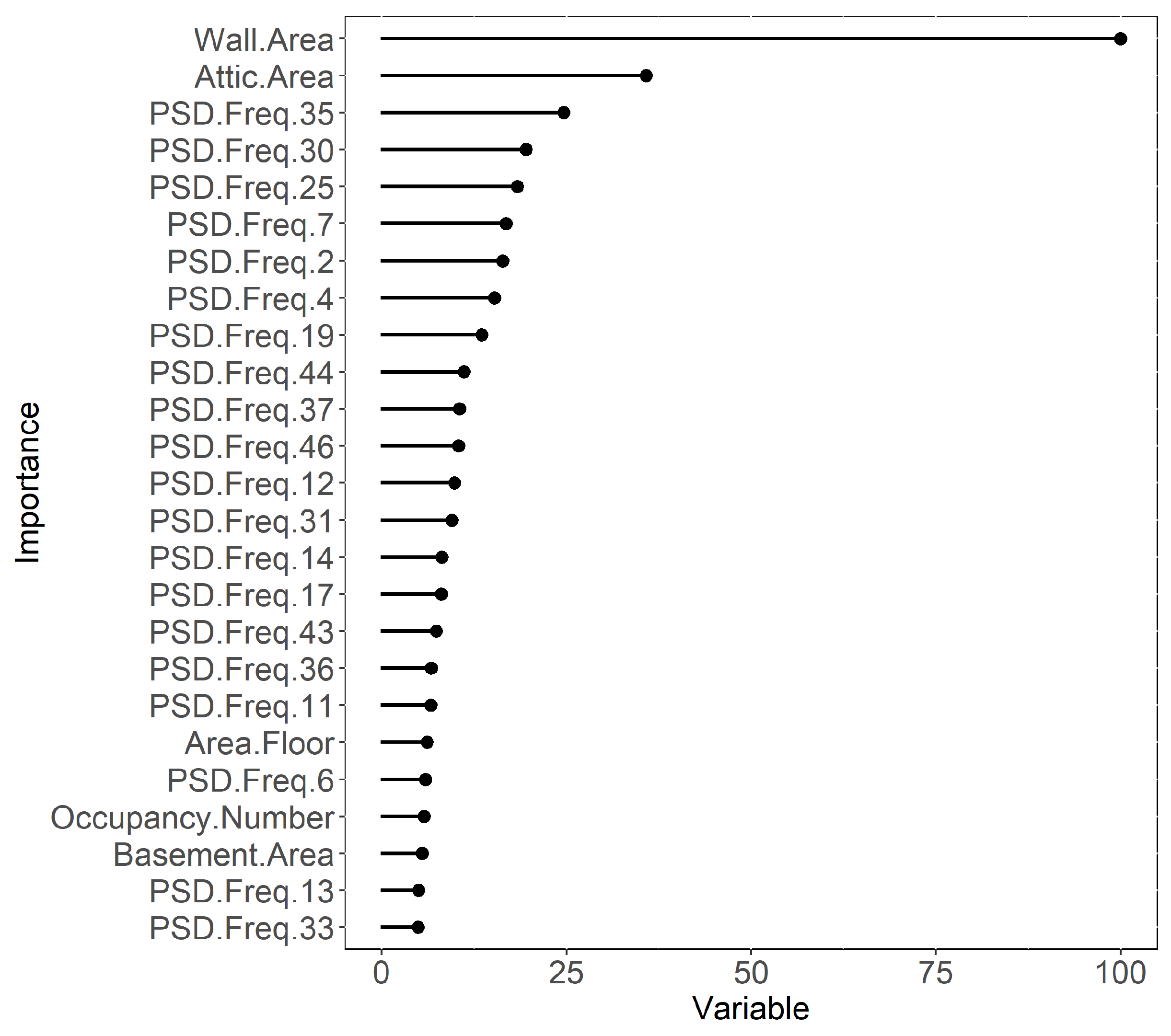
4.1. Assessing the Importance of Thermostat-Derived Data in Improving Prediction of Monthly Energy Consumption

First, all predictors (residential building geometry, energy characteristics, and occupancy, thermostat derived power spectra data, and monthly probability density of outdoor temperature) were considered in developing a singular model representing all residences in the study using the H2O AutoML toolkit [29] to predict the monthly gas consumption for all residences. A variable importance plot was developed for the best model obtained, shown in Figure 1. Of note in this figure is that while the geometrical characteristics associated with the wall and attic areas are deemed most important, the power spectrum features (indicated as PSD Freq.X) are also very important. In fact, a number of the frequency bins are deemed more important than energy characteristic features such as the attic and wall R-Values. Most importantly, these features can be derived from the thermostat data alone; potentially mitigating the need to collect energy characteristics for the residence from on-site assessments.

4.1.1. Development of Best Model to Predict Energy Consumption

The GBM model showed outstanding prediction accuracy.

Table 5. Feature selection cases with model prediction evaluation parameters for the testing dataset.

Case	Feature Types	R2	RMSE	MAE, Annual Gas Consumption (MJ)	MAPE
(a)	geometrical and outdoor temperature probability density bin	0.7533	2724.36	2319.08	0.2191
(b)	geometrical, outdoor temperature probability density bin, number of occupants, and energy system characteristics	0.8641	1993.98	1641.50	0.1644
(c)	geometrical, outdoor temperature probability density bin, number of occupants, energy system characteristics, and questionnaire	0.8646	1939.65	1602.43	0.1644
(d)	geometrical, outdoor temperature probability density bin, number of occupants, energy system characteristics, questionnaire, and all PSD bins	0.9109	1673.73	1413.29	0.1650
(e)	geometrical, outdoor temperature probability density bin, number of occupants, energy system characteristics, questionnaire, and top five PSD frequency bins (35, 30, 25, 7, and 2)	0.8867	1770.57	1415.60	0.1561
(f)	geometrical, outdoor temperature probability density bin, number of occupants, energy system characteristics, questionnaire, and six PSD frequency bins (6, 13, 16, 23, 24 and 46)	0.9519	1234.80	996.52	0.1465
(g)	geometrical, outdoor temperature probability density bin, number of occupants, questionnaire, and six PSD frequency bins (6, 13, 16, 23, 24 and 46)	0.8881	1728.65	1396.56	0.1586

shows the error metrics from the testing dataset for the best models developed using this machine learning algorithm for subsets of the input features available. The predictor subsets considered for model development are documented in the table below. Additionally included are the error metrics. The MAE and RMSE error metrics are based upon energy consumption for whole year. In this table, Case (a) includes as predictors only geometrical and outdoor temperature probability density bin values. Case (b) adds consideration of both number of occupants and energy system characteristics data. It is clear that the addition of these features improved the model performance considerably. Case (c) adds questionnaire data with regards to the presence of a washer/dryer and dishwasher. The addition of this data did little to improve the model. Case (d) adds all thermostat measured indoor temperature power spectrum data. Again, there is significant improvement in the model from these input features. Thus, thermostat data conclusively improves the ability to accurately model monthly energy consumption. Case (e) considers only the top five frequency bins of the power spectra information obtained from a variable importance analysis. The model performance actually deteriorates. Case (f) adds six frequency bins used to predict energy characteristics (attic R-Value, walls R-Value, furnace efficiency, and AC SEER) by Alanezi et al. [24]. These frequencies were shown in this prior study to best enable accurate prediction of the actual energy characteristics for a residence. The model performance for this case is seen to improve markedly; the R-squared value is 0.9519 and the MAE is 996.52. In Case (g) the energy characteristics and occupancy data are removed from this best model. The model performance is noted to have declined considerably. Thus, while the goal was to develop a model that would require no on-site collected data, it is clear that such data is valuable in terms of producing an accurate model for estimating energy consumption, and likewise energy savings (see Equation (6)).

Overall, the best model (case f) yielded an average residential consumption over this time frame of 11,463 MJ, associated with a mean error in predicting monthly energy consumption for all of the residences considered of ±8.69%. The associated R-squared value is 0.9519. This prediction is better than the best to date in terms of predicting monthly energy consumption (Altarhuni et al.; R-squared value = 0.94, [14]). It should be noted that Altarhuni’s approach used a regression of monthly energy data for each residence against monthly average outdoor temperature to derive predictors which could be used in a singular model to predict consumption of any residence. So, in effect, it used energy data to develop predictive features to predict energy consumption. The approach developed here does not do this.

4.1.2. Best Model Testing Results

The best model developed for Case f above, was tested on six residences not used in the training of the model. The testing results for these six residences are shown in

Table 6. Model prediction evaluation parameters for testing dataset.

Target	R2	RMSE	MAPE	MAE
Test House 1	0.9472	1406.42	0.1240	1073.18
Test House 2	0.9485	1306.15	0.0842	910.01
Test House 3	0.9725	913.75	0.0729	646.85
Test House 4	0.9201	1822.71	0.3276	1678.40
Test House 5	0.9788	743.02	0.1233	613.37
Test House 6	0.9446	1216.73	0.1470	1057.32
Average	0.9519	1234.80	0.1465	996.52

. The R-squared and MAE values for predicting the monthly natural gas usage were respectively 0.9472, 0.9485, 0.9725, 0.9201, 0.9788, and 0.9446 (R-squared), and 1073.18, 910.01, 646.85, 1678.40, 613.37, and 1057.32 MJ (MAE). These results illustrate that the model predictive effectiveness is consistent with the validation metrics used in the training, helping to establish the generalizability of the model to new residential data.

A time series plot of the monthly natural gas consumption as a function of time for the six test residences is shown in Figure 2. The figure compares both the actual and predicted consumption. It is clear that the two lines representing actual and predicted consumption correspond very well. Note that the actual and predicted values for each of the testing houses are shown in

Table A1. Actual and predicted data for 12 months of the testing houses using the best model.

Date	House 1		House 2		House 3
	Actual	Predicted	Actual	Predicted	Actual	Predicted
Oct-16	6414	7757	5762	6549	6088	5229
Nov-16	17,069	15,463	15,546	15,760	17,503	15,136
Jan-17	17,612	14,589	14,242	15,107	15,873	14,537
Feb-17	17,286	14,580	15,003	15,607	14,785	15,031
Mar-17	5544	6321	5436	5779	4892	4881
Aug-17	1956	2721	1848	1920	1195	1516
Sep-17	2283	2682	1630	1880	1630	1565
Oct-17	9784	9424	10,763	9229	7827	7796
Nov-17	14,894	14,825	18,699	15,162	13,155	12,821
Jan-18	19,569	19,127	16,851	18,465	15,220	14,417
Feb-18	16,742	15,693	15,220	15,303	13,807	13,157
Mar-18	13,916	13,578	14,242	13,224	12,720	11,980
Date	House 4		House 5		House 6
	Actual	Predicted	Actual	Predicted	Actual	Predicted
Oct-16	5762	8108	5762	6302	7066	5737
Nov-16	16,742	17,721	15,220	15,087	15,329	16,560
Jan-17	15,220	16,496	14,024	13,737	13,807	16,027
Feb-17	16,742	17,606	14,568	15,366	14,785	16,702
Mar-17	5979	7654	5218	6703	5762	6291
Aug-17	1304	3241	1630	2523	2935	1641
Sep-17	1739	3473	2065	2561	3152	1683
Oct-17	12,720	10,528	7066	7570	9567	8646
Nov-17	19,895	16,484	13,590	13,586	15,220	15,434
Jan-18	19,134	18,237	15,112	16,157	18,156	17,737
Feb-18	17,177	16,091	14,351	14,159	16,416	15,694
Mar-18	15,112	13,367	12,828	11,846	14,459	14,882

at the Appendix A section.

4.2. Estimating Savings and Quantifying Uncertainty in the Savings Predictions

As noted previously, two of the residents included in the study received upgrades in terms of attic insulation. The estimated energy savings for one month of these two residences using Equation (5) are shown in

Table 7. Savings percentage and uncertainty for an attic retrofit.

House Number	Bill Month Post-Retrofit	Measured Natural Gas Consumption (MJ)	Predicted Natural Gas Consumption Assuming no Upgrade (MJ)	Uncertainty in Estimating Consumption (MJ month−1)	% Savings	Uncertainty in Estimating Saving (%)
House 1	December 2019	14,677.20	18,712.95	±996.52	21.57	±4.18
House 2		11,415.60	13,476.24		15.29	±6.26

. The results indicate the natural gas consumption savings from attic insulation upgrade for House 1 and 2 are respectively 21.5% and 15.3%. Improvement to attic insulation in House 1 show significantly superior energy savings relative to House 2. The results are consistent with expectation, because House 1 no insulation prior to the upgrade, while House 2 had a very small amount of insulation. The uncertainty in the reported savings is respectively for House 1 and 2 ±4.18% and ±6.26%.

In an effort to generalize the results, the following questions are posed. What-if the energy savings is less? What percentage savings could we resolve? What percentage savings can be resolved?

Figure 3 shows a plot of the predicted savings (MJ) versus percentage savings for House 1 above were the actual savings to be less than that reported in Table 7. Error bars are shown to represent the uncertainty in predicting the savings (from Equation (5)). It is clear from this figure that as the percentage savings declines, the uncertainty in estimating savings increases slightly. It is also clear that accuracy in estimating savings declines. In fact, no savings can be resolved for savings percentages of less than roughly 5% based upon this approach. At this cut-off the uncertainty in estimating savings is approximately equal to the estimated savings. This savings resolution is valid for any residence, given that it derives from a model based upon a large number of residences. In comparison, the ASHRAE guideline for estimating savings from whole-building energy consumption at best renders an estimation of savings no less than 10% of total consumption. Thus, there is certainty that this approach renders substantial improvement in both the estimation accuracy of savings and the percentage savings which can be resolved.

5. Discussion and Conclusions

This research presents an improved accuracy approach to predict monthly natural gas consumption for residential buildings from accessible residential building information, historical weather data, and archived smart WiFi thermostat data utilizing a machine learning-based approach. The singular model developed using data from a collection of residences can be used to accurately predict consumption and savings from upgrades or changes in behavior for any residence with geometrical and energy characteristics represented within the minimum–maximum bounds of the features of the residences included in the training. Specifically the approach employed, because of the use of data derived from high frequency smart WiFi data, yields a mean error rate of ±8.69% for predicting annual consumption. Most significantly, for two houses for which insulation upgrades were implemented during the study period, savings estimation uncertainty was less than ±7%. This result shows the promise of the approach used here in estimating HVAC and envelope upgrades in any residence where monthly energy consumption is known, and smart WiFi thermostats are available. In fact, results are shown which demonstrate the ability to resolve energy savings of less than 5% for any residence. This is a big improvement upon the ASHRAE recommended guideline for estimating savings from whole-building energy consumption, where at best energy savings no less than 10% of total consumption can be resolved. It is expected that model improvement and therefore improvement in estimating both energy consumption and savings is possible through the addition of additional residential data.

With this technique, there is significant potential for implementing utility-scale programs to estimate consumption and measure savings from energy efficiency upgrades and/or behavior-based changes with accuracy. Precise savings estimates can help to validate value from all energy measures implemented in any house. The knowledge derived could help to inform more strategic energy reduction programs at a utility scale. Investment could be focused on measures having the potential for measurable savings.

Unfortunately, the results did not show that only remotely obtainable data were sufficient to yield high accuracy estimations of consumption and savings. The results showed a need to document wall and attic insulation amount and heating/cooling system efficiencies prior to an upgrade. This data likely requires on-site inspection.

Additionally, there are several notable limitations of this research and it can be future work to improve the study. First, it is necessary to expand the training dataset to contain a greater number of residences and more variety in the residences included. The current training data did not include very large and very small residences. Nor did it contain any stone, stucco, or brick residences. Second, the training data should use more behavioral information derive from smart WiFi thermostat including thermostat temperature set point history. Lastly, this approach was tested only in a single climatic region. In order to develop truly generalizable models applicable to anywhere, it is essential to broaden the location of the residences included in the singular model training data.

References

1. U.S. Energy Facts Explained. U.S. Energy Information Administration (EIA), 7 May 2020. Available online: https://www.eia.gov/energyexplained/us-energy-facts/ (accessed on 18 October 2020).
2. Amasyali, K.; El-Gohary, N.M. A review of data-driven building energy consumption prediction studies. Renew. Sustain. Energy Rev. 2018, 81, 1192–1205. [Google Scholar] [CrossRef]
3. Jacobson, M.Z.; Delucchi, M.A.; Bauer, Z.A.; Goodman, S.C.; Chapman, W.E.; Cameron, M.A.; Bozonnat, C.; Chobadi, L.; Clonts, H.A.; Enevoldsen, P.; et al. 100% Clean and Renewable Wind, Water, and Sunlight All-Sector Energy Roadmaps for 139 Countries of the World. Joule 2017, 1, 108–121. [Google Scholar] [CrossRef] [Green Version]
4. Haberl, J.S.; Culp, C.; Claridge, D.E. ASHRAE’s Guideline 14-2002 for Measurement of Energy and Demand Savings: How to Determine What Was Really Saved by the Retrofit. In Proceedings of the Fifth International Conference for Enhanced Building Operations, Pittsburgh, PA, USA, 11–13 October 2005. [Google Scholar]
5. Guideline 14-2002: Measurement of Energy and Demand Savings; ASHRAE: Atlanta, GA, USA, 2002.
6. Kissock, J.K.; Haberl, J.S.; Clarifge, D.E. Inverse Modeling Toolkit: Numerical Algorithms. ASHRAE Trans. 2003, 109, 425–434. [Google Scholar]
7. Inverse Modeling of Portfolio Energy Data for Effective Use with Energy Managers. In Proceedings of the 15th IBPSA Conference, San Francisco, CA, USA, 7–9 August 2017.
8. King, J. Energy Impacts of Smart Home Technologies; American Council for an Energy-Efficient Economy: Washington, DC, USA, 2018. [Google Scholar]
9. Lou, R.; Hallinan, K.P.; Huang, K.; Reissman, T. Smart Wifi Thermostat-Enabled Thermal Comfort Control in Residences. Sustainability 2020, 12, 1919. [Google Scholar] [CrossRef] [Green Version]
10. Huang, K.; Hallinan, K.P.; Lou, R.; Alanezi, A.; Alshatshati, S.; Sun, Q. Self-Learning Algorithm to Predict Indoor Temperature and Cooling Demand from Smart WiFi Thermostat in a Residential Building. Sustainability 2020, 12, 7110. [Google Scholar] [CrossRef]
11. Mosavi, A.; Bahmani, A. Energy consumption prediction using machine learning: A review. Preprints 2019. [Google Scholar] [CrossRef]
12. Seyedzadeh, S.; Rahimian, F.P.; Glesk, I.; Roper, M. Machine learning for estimation of building energy consumption and performance: A review. Vis. Eng. 2018, 6, 5. [Google Scholar] [CrossRef]
13. Villa, S.; Sassanelli, C. The Data-Driven Multi-Step Approach for Dynamic Estimation of Buildings’ Interior Temperature. Energies 2020, 13, 6654. [Google Scholar] [CrossRef]
14. Al Tarhuni, B.; Naji, A.; Brodrick, P.G.; Hallinan, K.P.; Brecha, R.J.; Yao, Z. Large scale residential energy efficiency prioritization enabled by machine learning. Energy Effic. 2019, 12, 2055–2078. [Google Scholar] [CrossRef]
15. Özmen, A.; Yılmaz, Y.; Weber, G.-W. Natural gas consumption forecast with MARS and CMARS models for residential users. Energy Econ. 2018, 70, 357–381. [Google Scholar] [CrossRef]
16. Iwafune, Y.; Yagita, Y.; Ikegami, T.; Ogimoto, K. Short-term forecasting of residential building load for distributed energy management. In Proceedings of the 2014 IEEE International Energy Conference (ENERGYCON), Cavtat, Dubrovnik, Croatia, 13–16 May 2014. [Google Scholar]
17. Li, Q.; Meng, Q.; Cai, J.; Yoshino, H.; Mochida, A. Applying support vector machine to predict hourly cooling load in the building. Appl. Energy 2009, 86, 2249–2256. [Google Scholar] [CrossRef]
18. Massana, J.; Pous, C.; Burgas, L.; Melendez, J.; Colomer, J. Short-term load forecasting in a non-residential building contrasting models and attributes. Energy Build. 2015, 92, 322–330. [Google Scholar] [CrossRef] [Green Version]
19. Kwok, S.S.; Yuen, R.K.; Lee, E.W. An intelligent approach to assessing the effect of building occupancy on building cooling load prediction. Build. Environ. 2011, 46, 1681–1690. [Google Scholar] [CrossRef]
20. Jovanovic, R.Z.; Sretenovic, A.A.; Zivkovic, B.D. Ensemble of various neural networks for prediction of heating energy consumption. Energy Build. 2015, 94, 189–199. [Google Scholar] [CrossRef]
21. Zhao, D.; Zhong, M.; Zhang, X.; Su, X. Energy consumption predicting model of VRV (Variable refrigerant volume) system in office buildings based on data mining. Energy 2016, 102, 660–668. [Google Scholar] [CrossRef]
22. Li, Q.; Ren, P.; Meng, Q. Prediction Model of Annual Energy Consumption of Residential Buildings. In Proceedings of the 2010 International Conference on Advances in Energy Engineering, Beijing, China, 19–20 June 2010. [Google Scholar]
23. Ekici, B.B.; Aksoy, U.T. Prediction of building energy consumption by using artificial neural networks. Adv. Eng. Softw. 2009, 40, 356–362. [Google Scholar] [CrossRef]
24. Alanezi, A.; Hallinan, K.P.; Brodrick, P.G.; Huang, K. Interviewees, Automated Residential Energy Audits Using a Smart WiFi Thermostat Enabled Data Mining Approach. Energy Build. 2021. [Google Scholar]
25. National Oceanic and Atmospheric Administration (NOAA). U.S. Department of Commerce. Available online: https://gis.ncdc.noaa.gov/maps/ncei/ (accessed on 16 August 2018).
26. Chakrabarty, A.; Mannan, S.; Çagin, T. Inherently Safer Design. In Multiscale Modeling for Process Safety Applications; Butterworth-Heinemann: Oxford, UK, 2016; pp. 339–396. [Google Scholar]
27. Drori, I.; Liu, L.; Nian, Y.; Koorathota, S.C.; Li, J.S.; Moretti, A.K.; Freire, J.; Udell, M. AutoML using Metadata Language Embeddings. In Proceedings of the 33rd Conference on Neural Information Processing Systems, Vancouver, BC, Canada, 8–14 December 2019. [Google Scholar]
28. Osman, H.; Ghafari, M.; Nierstrasz, O. Hyperparameter optimization to improve bug prediction accuracy. In Proceedings of the 2017 IEEE Workshop on Machine Learning Techniques for Software Quality Evaluation, Klagenfurt, Austria, 21 February 2017; pp. 33–38. [Google Scholar]
29. AutoML: Automatic Machine Learning. H2O.ai, 18 June 2020. Available online: https://docs.h2o.ai/h2o/latest-stable/h2o-docs/automl.html (accessed on 19 June 2020).
Figure 1. Variable importance plots including thermostat derived information for natural gas consumption model.
Energies 14 00187 g001
Figure 2. Time series natural gas energy consumption plots for each of the testing houses: (a) House 1; (b) House 2; (c) House 3; (d) House 4; (e) House 5; and (f) House 6.
Energies 14 00187 g002
Figure 3. Plot of savings (MJ) versus percentage savings for House 1 with error bars associated with the uncertainty in estimating savings.
Energies 14 00187 g003