Abstract
Electromagnetic interference (EMI) from renewable power systems to the grid attracts more attention especially in the low-frequency range, due to the low switching frequency of high-power inverters. It is significantly important to derive EMI models of power inverters as well as to develop strategies to suppress the related conducted emissions. In this work, black-box modelling is applied to a three-phase inverter system, by implementing an alternative procedure to identify the parameters describing the active part of the model. Besides, two limitations of black-box modelling are investigated. The first regards the need for the system to satisfy the linear and time-invariant (LTI) assumption. The influence of this assumption on prediction accuracy is analysed with reference to the zero, positive and negative sequence decomposition. It is showing that predictions for the positive/negative sequence are highly influenced by this assumption, unlike those for the zero sequence. The second limitation is related to the possible variation of the mains impedance which is not satisfactorily stabilized at a low frequency outside the operating frequency range of standard line impedance stabilization networks.
1. Introduction
With the widespread of renewable energy technologies, such as photovoltaic (PV) panels and wind farms, the development of a suitable tool to predict and reduce the conducted emission (CE) generated by renewable power systems has gained increasing attention from the Electromagnetic Compatibility (EMC) community due to the severe electromagnetic interference (EMI) threats these noise currents can cause when propagating through the power grid [1]. Indeed, they can be responsible for interference with consequent malfunctioning in smart communications and metering systems [2], thus reducing the reliability and interoperability of the whole infrastructure. Particularly, since the switching frequencies of most high-power converters are still limited to a few kHz only [3,4], these applications have brought to the attention of the community the partial lack of regulations in the frequency interval between 2 kHz (maximum frequency foreseen by International Power Quality Standards) and 150 kHz (minimum frequency foreseen by International EMC Standards) [5,6,7], which is covered (often only partially) by a few of Standards for specific applications only [8]. In this frequency interval, also the availability of devices suitable to run the required measurement and tests is limited. An explicative example is the Line Impedance Stabilization Network (LISN), whose use in EMC test setups is fundamental to assure that the CEs exiting the device under test were measured on a stable impedance, despite possible variations of the mains impedance. Topology and values of LISN components depend on the specific Standards and are selected to ensure the correct operation of the LISN in the frequency interval foreseen by the Standards. For instance, the LISN layout specified in the International Special Committee on Radio Interference (CISPR) 22 Standard is different from the one recommended by the CISPR 16 Standard, as they are expected to cover two different frequency intervals: The former from 150 kHz to 30 MHz, the latter from 9 kHz to 30 MHz. Using the LISN outside its recommended frequency range may jeopardize test repeatability leading to unpredictably different CE levels.
In this respect, developing effective strategies to model power converters is relevant not only in view of predicting the generated CE and of deriving guidelines to design proper countermeasures (e.g., design of suitable passive, active, or hybrid EMI filters) but also in view of developing new test setups, procedures, and measurement devices to supplement the regulations currently available in the Standards and to extend their applicability starting from lower frequencies (i.e., 2 kHz or lower).
The challenge is to derive power converter models able to represent not only the functional part of the system (i.e., the switching activity of the power modules along with their control system) but also all those undesired mechanisms and parasitic paths leading to the generation and propagation of the CE exiting the converter. In the literature, either circuit models for time-domain analysis and behaviour models for frequency-domain analysis can be found [9,10]. The former approach is definitely more flexible since it involves an explicit circuit representation of the functional and parasitic behaviour of the converter. However, it usually requires detailed knowledge of the internal structure of the converter along with a huge effort to identify suitable setups and procedures to extract from the measurement data (or from the manufacturer data-sheets) proper values for the involved circuit components. Moreover, this approach may be scarcely effective when time-domain simulation of complex systems is the target, since the complexity of the obtained network may rise to convergence issues [11].
Behavioural modelling strategies can help to overcome most of the aforesaid limitations. This latter approach foresees to provide the converter with a black-box representation at the output ports in terms of an equivalent Thevenin/Norton circuit. The obtained “black-box” model involves a minimum number of active and passive components, whose frequency response is extracted from measurements carried out at the output ports of the converter. Although such a black-box approach does not offer any flexibility in the modelling of the converter control system, it is definitely beneficial for EMC analyses in complex systems. Indeed, it does not require any knowledge about the internal structure of the converter, since measurements at the external ports only are required to derive the frequency response of the involved model parameters [10].
The theoretical assumption behind this approach is that the device under analysis can be treated (at least approximately) as a linear and time-invariant (LTI) system. However, since switching modules exhibit an inherently time-variant and non-linear behaviour, a thorough investigation aimed at identifying the conditions for applicability and possible limitations of black-box modelling is required.
For this purpose, the black-box modelling technique in [12], which was originally adopted for modelling DC-DC converters in a satellite power system, is extended in this work. The model aims to predict the CE peaks related to the switching frequency and its harmonics exiting the AC side of a three-phase inverter connected to a PV panel. For the proposed modelling procedure, accuracy, applicability, and possible limitations of black-box modelling are systematically investigated, by paying particular attention to the low-frequency part of the spectrum down to 2 kHz (since the switching frequency of the inverter here considered is 5 kHz). To this end, an explicit model of the whole system (i.e., a model involving the switching modules, the control system as well as parasitic components) is preliminarily implemented in SPICE (it stands for Simulation Program with Integrated Circuit Emphasis) and used as a virtual environment to emulate the steps of the proposed experimental procedure and to obtain a prediction of the generated CE to be used as a reference to validate the proposed modelling strategy.
The accuracy of the obtained CE prediction is analysed not only in terms of physical voltages measured at the LISN output but also in terms of modal quantities. To this end, the decomposition of physical quantities into positive, negative and zero-sequence components is adopted, which is the one usually exploited in power systems analyses. Particular attention is devoted to investigating the influence on model effectiveness of the presence of a so-called mask impedance (here, the output filter installed at the ac-side of the inverter) as well as the bandwidth of the LISN exploited in the setup for model parameter extraction (active part).
The rest of the manuscript is organized as follows. Section 2 surveys the black-box modelling strategies available in the literature and discusses the LTI assumption. Section 3 describes the inverter system under analysis and introduces the test setups and procedures proposed for model-parameter extraction from measurement data. The accuracy of the proposed modelling technique is investigated in Section 4, by comparing the prediction obtained by the black-box model with those obtained by SPICE simulation of the whole system. Also, in this section possible limitations of the proposed approach are investigated and discussed. Conclusions are eventually drawn in Section 5.
2. Black-Box Modelling Procedures and LTI Assumption
2.1. Black-Box Modelling Procedures
In the literature, there are mainly two methods to extract black-box models of power converters. In one approach, a set of independent tests are carried out by connecting suitable external networks of known impedance to write and solve suitable equations involving the unknown parameters of the black-box model. The number of terminals of the system under analysis determines the topology of the obtained model (i.e., number of required impedances and sources) as well as the number of configurations [13]. For example, the black-box model of a DC/DC converter with three terminals (phase, neutral and ground) can be represented by five unknowns (i.e., two sources and three impedances). This means that at least three different measurement configurations are needed to write five linearly independent equations for the voltages/currents measured in each of the three setups [9]. The use of three setups leads to an overdetermined system of six equations in five unknowns, which can be solved by adopting, e.g., least-square algorithms [14].
An alternative approach is to separately characterize the active part (noise sources) and the passive part (impedance/admittance matrices) of the model. For the characterization of the passive part, most of the methods available in the literature foresee impedance measurement with the converter switched off through Impedance or Vector Network Analyzer (VNA) [15]. For instance, the method in [12] involves the use of a VNA to measure the scattering parameters then converted into admittances with the converter off, (see Figure 1a). Besides, the current sources are obtained starting from the measurement of output currents of the converter by connecting the converter to the power network through a LISN required by the standard measurement setups of conducted emissions. Moreover, alternative indirect measurement such as the so-called ‘insertion loss’ method [16] and analytical calculation method [17] are also investigated in some papers.
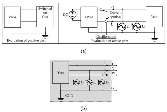
Figure 1.
(a) Principle drawing of the black-box modelling technique in [12]: Identification of passive (left panel) and active (right panel) parameters separately. (b) Black-box model of the three-phase inverter system.
Approaches based on separate evaluation of the active and passive part (Figure 1a) seem to be more promising because (1) they require only two measurement setups, (2) the extraction of the unknown parameters from measurement data does not involve the solution of a system of overdetermined equations. This is a great advantage in terms of accuracy of the results as post-processing of the measurement data can often introduce significant numerical errors which degrade the accuracy of the extracted model.
For these reasons, black-box modelling procedures evaluating the parameters of the active and passive parts of the model separately (Figure 1a) are adopted in this work and extended to a three-phase grid-connected inverter system. The extracted black-box model is shown in Figure 1b (Norton equivalent circuit) and it involves an admittance matrix and three current sources. The passive part of the model is evaluated by VNA measurement. The evaluation of the noise current sources is carried out with a LISN (instead of current probes) to avoid measurement uncertainty due to the presence of a fundamental 50 Hz component on the AC side of the inverter.
2.2. LTI Assumption
Black-box modelling provides an equivalent frequency-domain representation (in terms of the Thevenin/Norton circuit) at the external ports of the device to be modelled. Consequently, the applicability and effectiveness of this strategy are limited to the modelling of linear and time-invariant devices only. Since power converters are intrinsically non-linear and time-variant networks, black-box modelling requires preliminary verification that the device can be treated, at least approximately, as an LTI system. Indeed, if the system does not satisfy the LTI assumption, the use of different operating conditions to identify model parameters could lead to different black-box models, which makes the models unsuited to assure accurate predictions with other operating conditions.
In this regard, further investigations are needed to verify when and under what conditions it is possible to apply black-box modelling approaches for modelling power converters. In several works [18,19,20], such an assumption was assumed to be satisfied, since the converter under analysis was equipped with an EMI filter or decoupling capacitors/functional inductors, which can mask the inherently non-linear and time-varying behaviour of the switching modules.
However, this conclusion cannot be a priori extended to all power converters. For instance, in [21] it was experimentally observed that, unlike the common-mode (CM) impedance (whose frequency response is dominated by parasitic effects), the differential model (DM) impedance can exhibit a different frequency response depending on the on or off status of the converter. In these cases, extracting the parameters of the black-box model with the converter switched off may significantly impair prediction effectiveness and accuracy.
3. Identification of Model Parameters in a Virtual Test Bench
3.1. Inverter System under Analysis
Without loss of generality, a three-phase inverter connecting a photovoltaic panel to the power grid, along with an LCL (i.e., inductor-capacitor-inductor) filter is considered as a system under analysis. The principle drawing of this system is illustrated in Figure 2. Though a single-stage inverter system is investigated in this paper, it is worth mentioning that DC/DC converters are frequently added between the PV array and the inverter for DC-link voltage control and maximum power point tracking. The presence of this additional converter is disregarded here for the sake of simplicity as its possible presence is not expected to impact the accuracy of the proposed modelling procedure as long as the LCL filter is installed at the AC side of the inverter.
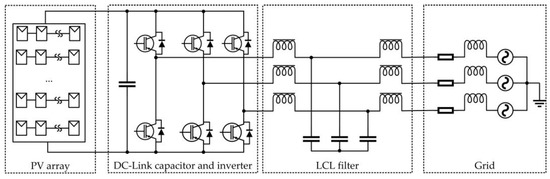
Figure 2.
Principle drawing of a grid-connected three-phase inverter system.
The complete circuit model of this system, including functional parts and parasitic components, will be implemented in SPICE and used as the reference circuits. The circuit models of each component in the system will be discussed in the following paragraphs.
The solar panel Photowatt Technologies (Isère, France) PW 1650-24 V, whose parasitic parameters are adopted from [22], is used to construct the PV array for the system. In this work, the PV array contains 32 PV panels in series to provide the proper DC power supply.
The complete circuit model of one Insulated-Gate Bipolar Transistor (IGBT) switching leg (SKM200GB122D) and the capacitors at the DC side are shown in Figure 3a [23]. One 1.5 mF electrolytic capacitor and one 0.33 µF ceramic capacitor are connected at the input of each inverter leg, respectively—The functional model is augmented by including the following parasitic components: Stray inductances (Lwa, Lw) and resistance (Rwa) of the connecting wires, parasitic inductances (LEL, Ls) and resistances (Rd, REL, Rs) of the DC capacitors, the stray inductances (Lc, LE), the gate resistance (RG) and internal capacitances (Cgc, Cge and Cce) of the IGBT/Diode devices (which are included in the SPICE models). Numerical values of the circuit elements in Figure 3a are collected in Appendix A (Table A1). The conventional Pulse-Width Modulation (PWM) strategy is implemented in SPICE with a 5 kHz switching frequency.
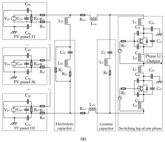
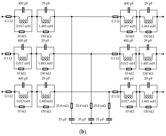
Figure 3.
Circuit model of (a) the inverter with input capacitors and (b) the LCL filter.
Grid-connected converters usually require an L or LCL filter attached at the output to reduce the harmonic currents in compliance with IEEE Standard 519–1992 and P1547-2003 requirements [24]. The LCL filter here adopted (see Figure 3b) was designed following the procedures in [25]. Relevant parameters are listed in Table A2 of Appendix A. Specifically, the equivalent circuit in [26] is adopted for the inductors, and datasheets are used to infer suitable values for the equivalent series resistance of the capacitors.
It is worth mentioning that from the viewpoint of black-box modelling, such an LCL filter also plays a fundamental role in masking the nonlinear and time-varying behaviour of the inverter, thus making the LTI assumption generally satisfied. This property will be investigated in the following, by comparing the CEs predicted in the presence and absence of the LCL filter.
Eventually, the power grid is modelled by the use of three sinusoidal voltage sources (properly shifted in phase) connected in series with three impedances, obtained as the series connection of a 1 Ω resistor and a 0.2 mH inductor to mimic typical (average) mains impedance values.
3.2. Black-Box Modelling
The procedure here exploited to identify black-box model parameters involves two different setups. The former is used to evaluate the entries of the admittance matrix (passive part of the model), the latter to extract the frequency response of the noise (current) sources (the active part of the model).
3.2.1. Passive Part of the Black-Box Model
As the first step, the entries of the admittance matrix Ydut are characterized through Vector Network Analyzer (VNA) measurement of the scattering parameters (S-parameter) at the output port of the LCL filter, as shown in Figure 4. For measurement, the gate signals and the DC-link voltage supply should be disconnected from the inverter for safety reason. To mimic VNA measurement conditions by the SPICE model, both the DC voltage sources and the gate signals sources are replaced by short circuits. The obtained 3 × 3 S-parameter matrix (Sdut) is then converted into the corresponding 3 × 3 admittance matrix Ydut by post-processing of measurement data [27].
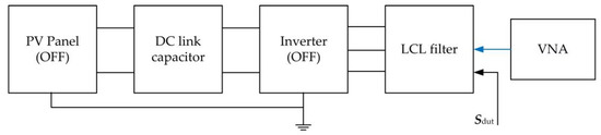
Figure 4.
Measurement setup exploited to evaluate the entries of the admittance matrix (passive part of the black-box model).
To implement this step of the identification procedure in SPICE [28], VNA operation is mimicked through the blocks shown in Figure 5. In the specific configuration shown in the figure, the active VNA port is connected between phase 1 and ground, the other phases being connected to 50 Ω loads, and the entries of the first column of the S-parameter matrix Sdut (i.e., parameters S11, S21 and S31) are evaluated. Subsequently, exchanging the position of such an active port to phase 2 and phase 3 allows measuring the entries of the second (S12, S22 and S32) and the third column (S13, S23 and S33), respectively.
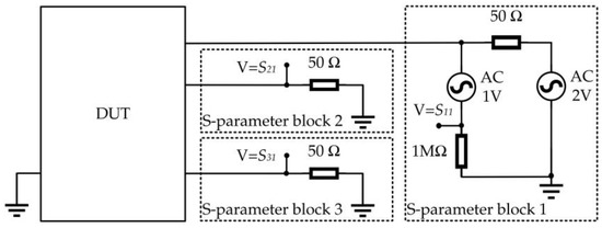
Figure 5.
SPICE implementation of the measurement setup used to evaluate the passive part of the model: The three blocks connected at the DUT ports are used to emulate the three ports of a VNA.
3.2.2. Active Part of the Black-Box Model
To extract from measurements the frequency response of the current sources Is1, Is2, and Is3 (active part of the black-box model), the test setup in Figure 6 is exploited. The voltages V4, V5, and V6 at the LISN output are measured in the time domain by the three channels of an oscilloscope (to obtain simultaneous measurements on the three phases), and then converted into the frequency domain by the Fourier Transform (FT).
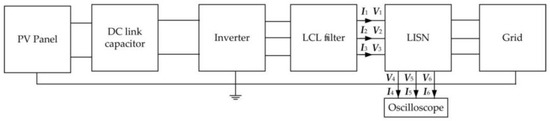
Figure 6.
Measurement setup exploited to evaluate the active part of the black-box model, i.e., the three current sources IS1, IS2 and IS3.
When the black-box modelling approach is applied to the DC side to assess CEs to PV panels, current probes can be used to measure the currents directly (see Figure 1a). This approach was carried out in [12] to build the black-box model of a DC/DC converter and was validated by experiment.
With respect to [12], where the noise sources were directly extracted from the currents measured at the converter input (Figure 1a), the procedure proposed here requires additional efforts in terms of post-processing, since the LISN should be preliminarily characterized as a six-port network by VNA measurement (yielding a 6 × 6 S-parameter matrix, SLISN), and its effect should be de-embedded from the measurement data.
However, this solution is preferable when time-domain measurements are to be carried out at the AC side of the inverter, as it allows filtering out the fundamental 50 Hz component, whose presence could cause inaccurate sampling of higher spectral components.
In SPICE, the aforesaid setup was implemented by connecting 50 Ω resistors at the LISN output ports to emulate the oscilloscope channels. Additionally, to preliminarily characterize the LISN in terms of six-port network, the blocks already introduced in Figure 5 are connected on both sides of the LISN, with the active block connected to one of the six ports at a time, to evaluate the entries of the 6 × 6 S-parameter matrix, SLISN. In this step, it has to be carefully considered that the impedance connected at the output port of the LISN may influence the results for frequencies outside the LISN bandwidth. As it will be shown in Section 4, this effect is mostly visible in the low-frequency part of the spectrum, since several LISNs are designed to comply with EMC standards foreseeing CE measurement starting from 150 kHz.
Once this matrix is known, voltages (V1, V2, V3) and currents (I1, I2, I3) at the DUT side of the LISN are computed as
where ABCDLISN is the 6 × 6 ABCD matrix of the LISN, obtained starting from the corresponding S-parameters matrix SLISN [27]. Eventually, the noise currents in the black-box model are retrieved as:
The magnitude of the extracted black-box-model parameters, i.e., the entries of the Y matrix and the three current sources, is plotted in Figure 7. The first plot, Figure 7a, shows the frequency response of DUT admittances: Due to the symmetry, diagonal entries are the same (Y11 = Y22 = Y33) as well as off-diagonal entries (Y12 = Y13 = Y23). Due to symmetry, also the frequency response of the three current sources is coincident, as shown in Figure 7b.
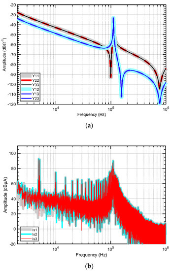
Figure 7.
Extracted black-box model: (a) Selected six Y-parameter of DUT; (b) Three current sources.
It is worth mentioning that LISN effectiveness in stabilizing the impedance seen from the DUT outlets in the whole frequency interval of interest is fundamental for model-parameter extraction. Indeed, since the LISN is connected with the mains for CE measurement, its effectiveness in providing a stable impedance, despite possible variation of the mains impedance, determines the accuracy of the noise-source extraction. Hence, to better investigate this specific aspect, in this work the two LISNs shown in Figure 8 will be considered, which are designed according to the requirements specified in the standard CISPR22, Figure 8a, and CISPR16, Figure 8b, respectively.
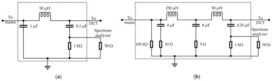
Figure 8.
Schematics of the two LISNs considered in this work: (a) CISPR22 and (b) CISPR16-1-2.
3.3. Setup for Model Validation
To effectively validate the accuracy of the obtained black-box model, the conducted emissions exiting the converter under loading conditions sufficiently different from those exploited for model-parameter identification, Figure 6, are to be predicted and compared versus those obtained by exploiting the explicit model of the converter (here used as reference quantities). To this end, an additional EMI filter, Figure 9a, is included between the system and the LISN to appreciably modify the converter working conditions despite the presence of the LISN. The obtained measurement setup is shown in Figure 9b.
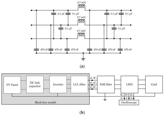
Figure 9.
Validation of the black-box model: an additional EMI filter (a) is included in the measurement setup (b) to modify the working conditions of the converter.
4. Prediction of Conducted Emissions
4.1. Conducted Emissions Analysis
As the first step, the conducted emissions exiting the inverter are evaluated in the presence and the absence of the EMI filter in terms of voltages measured at the output (i.e., at the receiver side) of a LISN compliant with CISPR16 specifications. To this end, time-domain simulations are carried out in SPICE, and the frequency spectra of the voltages at the LISN output are obtained afterwards through FT.
The conducted emissions simulated in the absence of the EMI filter are then used as input data to extract the black-box model of the inverter. Conversely, the conducted emissions simulated in the presence of the filter are used to assess the effectiveness of the extracted black-box model in predicting the emissions exiting the inverter under analysis, in combination with a different set of working conditions.
To verify the suitability of the aforesaid two sets of working conditions in assessing the prediction effectiveness of the extracted black-box model, the conducted emissions from the converter in the presence and in the absence of the EMI filter are preliminary compared in Figure 10 (where the voltage V4 on a specific phase is plotted). The significant difference between the two spectra confirms the effectiveness of introducing the EMI filter to generate a new set of working conditions for validation purposes. Apart from the first two spectrum lines at 5 kHz and 10 kHz, the EMI filter provides appreciable attenuation to all the other harmonics.
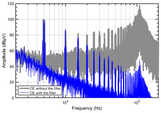
Figure 10.
Conducted emissions at the AC side of the inverter in the presence and in the absence of the EMI filter.
Moreover, modal decomposition is applied to get a better understanding of the spectral content of the emissions exiting the converter. To this end, the three-phase voltages V4, V5, V6 at the LISN output are decomposed into the corresponding positive-sequence, negative-sequence, and zero-sequence voltages V+, V−, V0 by the similarity transformation, [29]:
In this regard, it is worth mentioning that for EMC analysis decomposing phase quantities (voltages and currents) into CM and DM components is a standard practice, which allows the designer to identify the noise component that is dominant in a specific frequency interval, so to properly design the required EMI filter. For a three-phase system, the transformation into positive/negative/zero sequences in (3) provides equivalent information in terms of CM (zero sequences) and DMs (positive and negative sequences) noise components, and it is here adopted since it is widely adopted also for power system analysis. Since the similarity transformation matrix in (3) is not singular, phase voltage (V4, V5, V6) can be also obtained from modal quantities (V+, V−, V0), by reversing (3).
One of the phase voltage (V4) and the obtained modal voltages evaluated in the absence and the presence of the EMI filter are plotted in Figure 11a,b, respectively. The comparison versus the corresponding phase voltages (see the grey spectrum in Figure 11) reveals that the emissions from the converter are dominated by the positive and negative-sequence contributions up to nearly 35 kHz. Conversely, above this frequency the zero-sequence contribution is dominant. This result proves that the observed reduction of the converter CEs above 35 kHz is mainly to be ascribed to the effectiveness of the exploited EMI filter in damping the zero-sequence component of the noise currents exiting the converter.
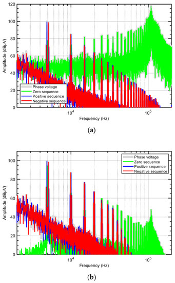
Figure 11.
Decomposition of the inverter CEs into positive, negative and zero-sequence components: (a) without the EMI filter; (b) with the EMI filter.
4.2. Validation of the Modelling Procedure
The conducted emissions obtained by the SPICE model of the whole test setup described in Section 3 and those predicted by the black-box model are compared in Figure 12a in the frequency range from 2 kHz to 200 kHz. The CEs above 200 kHz are not plotted, as they are significantly attenuated (below −10 dBµV). The comparison proves that the black-box model can effectively predict the emissions exiting the converter, with maximum deviations within 3 dB around 110 kHz, where the system exhibits a resonance.
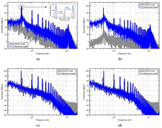
Figure 12.
Conducted emissions obtained by the SPICE model in Section 3 and predicted by the black-box model (a) phase voltage (b) zero-sequence voltage (c) positive sequence voltage and (d) negative sequence voltage.
The corresponding comparison in terms of zero sequence and positive/negative sequence is shown in Figure 12b–d, respectively, and confirms the effectiveness of the proposed black-box model also in predicting modal quantities. The zero-sequence and the positive/negative sequences dominate above and below 35 kHz, respectively. The discrepancies observed above 100 kHz are mainly owing to numerical processing of data, due to the extremely low CE levels at high frequency.
4.3. Limitations of Black-Box Modelling
4.3.1. Influence of the Mask Impedance
To investigate the role of the masking effect due to the LCL filter on model effectiveness, the LCL filter was removed, and the procedure for model parameter extraction was repeated. The obtained predictions are compared versus SPICE simulations in Figure 13a.
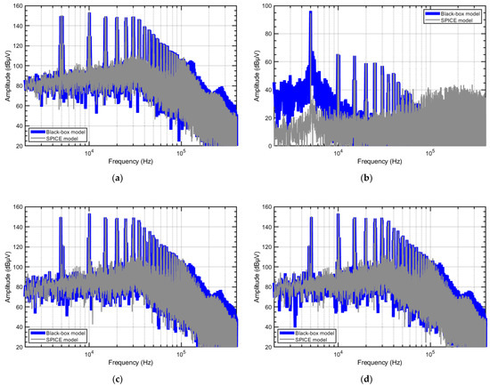
Figure 13.
Conducted emissions in the absence of LCL filter obtained by SPICE model in Section 3 and predicted by the black-box model (a) phase voltage (b) zero-sequence voltage (c) positive sequence voltage and (d) negative sequence voltage.
Specifically, for the system without the LCL filter, obvious mismatches are observed in predictions of CEs obtained by the black-box model from 100 to 400 kHz with respect to the accurate circuit simulation. In Figure 13b–d, three sequences of emissions are compared. It is observed that the discrepancies in this frequency interval are mainly from the positive and negative sequences instead of the zero sequence. With respect to Figure 12, the discrepancies observed in Figure 13 are to be ascribed to the inaccuracy of black-box modelling in the absence of the LCL filter, rather than to the noise floor of data-processing. As a matter of fact, in Figure 13 CE levels from 100 kHz to 400 kHz are still significantly larger (above 40 dBμV) than the noise floor.
This investigation puts in evidence that in the absence of an LCL filter (and its masking effect), the nonlinear and time-variant characteristics reflect the prediction of positive/negative sequence components. In this case, the black-box modelling approach is less accurate in the prediction of DM emissions, especially in the high frequency range.
4.3.2. Influence of the Power Network Impedance
For model-parameter evaluation, the ability of the exploited LISN in providing a stable impedance despite the possible variation of the impedance of the power grid plays a fundamental role. To extract the frequency response of the noise sources, the exploited LISN has to be disconnected from the power grid and preliminarily characterized by VNA measurements. At this stage, the impedance at the output port of the LISN (open-ended) is different from the actual impedance of the power grid (here mimicked by the series connection of a 0.2 mH inductor and a 1 Ω resistor), which is connected at the LISN output when noise currents are measured. Hence, if the LISN is used outside its bandwidth, the input impedance seen from its input port might be significantly different in the two test setups.
To investigate this specific aspect, different impedance values are assumed for the power grid, and the impedance seen at the input of the CISPR16 and CISPR22 LISNs are plotted in Figure 14a,b, respectively. The plots show that for frequencies below the LISN operation frequency range (i.e., for frequencies below 150 kHz for the CISPR22 LISN, and below 9 kHz for the CISPR16 LISN) non-negligible variations are observed in the impedance seen at the LISN input. This significantly impacts on CE measurement in the lower part of the spectrum, as shown in Figure 15, where the CEs measured by the two LISNs under analysis are compared (for these simulations the presence of the power grid was mimicked by the series connection of a 0.2 mH inductor and a 1 Ω resistor). The comparison shows significant differences in the measured CE levels for frequencies below 40 kHz, with maximum deviation in the order of 30 dB around 25 kHz.
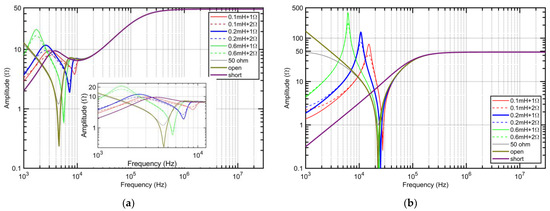
Figure 14.
Input impedance of the LISN for different impedances of the power grid attached at the output port: (a) CISPR16; (b) CISPR22 LISN.
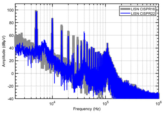
Figure 15.
Conducted emissions (SPICE model) measured by using two different LISNs, i.e., CISPR16 (grey spectrum) and CISPR22 (blue spectrum).
To investigate the influence of the exploited LISNs on the effectiveness of the proposed black-box modelling procedure, the two LISNs under analysis were preliminarily characterized in terms of scattering parameters with the output port left open-ended. As previously observed, this configuration reproduces the experimental setup involving the VNA and the LISN disconnected by the power grid.
After that, the CEs exiting the systems were virtually measured by exploiting the two LISNs connected to the power grid (emulated by the series connection of a 0.2 mH inductor and a 1 Ω resistor), and the obtained CE levels were used as input data to determine the frequency response of the noise sources involved in the black-box model.
The CEs predicted by the obtained black-box models are compared versus those predicted by the SPICE model in Figure 16. The comparison shows that the predictions obtained by exploiting the CISPR16 LISN exhibit a deviation (less than 3 dB) at the switching frequency (5 kHz) only. Conversely, if the black-box model is extracted by exploiting the CISPR22 LISN, the predictions reveal significant deviations with respect to SPICE simulation below 150 kHz, since such a LISN is designed to assure a stable impedance starting from 150 kHz only.
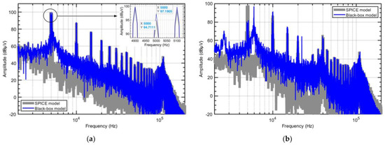
Figure 16.
CE levels predicted by exploiting two different LISNs, i.e., (a) CISPR16 and (b) CISPR22 LISN: SPICE versus black-box model.
5. Conclusions
In this work, the effectiveness and possible limitations of a black-box modelling procedure tailored to the representation of a three-phase inverter connected with a PV panel have been investigated. The procedure foresees separate characterization of the active and passive part of the model. Specifically, a suitable procedure is proposed to identify the noise sources (active part of the model), which resorts to the time-domain measurement of the voltages at the output of the LISN, instead of the currents exiting the converter, to filter out the 50 Hz fundamental component, whose contribution could impair the identification of higher frequency components. The comparison versus SPICE simulation proved the effectiveness of the proposed black-box modelling approach in predicting the CEs exiting the AC side of the grid-tied three-phase inverter system under analysis in the frequency range starting from 2 kHz.
The proposed analysis allowed a systematic investigation of two main limitations possibly degrading the prediction accuracy of the proposed black-box modelling technique during the measurement. The former limitation is related to the assumption that the system under analysis should be treated, at least approximately, as a linear and time-invariant system. In this regard, the fundamental role played by the LCL filter (installed at the converter output) in masking the inherent non-linear and time-invariant behaviour of the inverter switching modules has been proven. In general, this assumption needs to be confirmed prior to the application of the black-box modelling procedures. The latter limitation is related to the bandwidth of the LISN exploited to extract from measurement the frequency response of the noise sources (active part of the model). In this regard, it has been proven that using a LISN foreseen for CE measurement starting from 150 kHz, as foreseen by several EMC standards, may lead to significant degradation of prediction accuracy in the lower part of the spectrum (i.e., below 150 kHz), since the frequency response of the extracted noise sources is strongly influenced by the impedance connected at the output of the LISN. To eliminate the influence of power network impedance, it is necessary to develop a new type of LISN with stable impedance starting from 2 kHz, otherwise, the mains impedance must be measured or estimated to improve the accuracy of the black-box model predictions at low frequency.
Author Contributions
Conceptualization, M.Z., L.T., R.C. and S.A.P.; methodology, F.G. and G.S.; software, L.W. and A.H.B.; validation, X.W., X.L.; formal analysis, F.G., X.W. and L.W.; investigation, G.S., A.H.B. and L.W.; resources, M.Z., L.T. and F.G.; writing—original draft preparation, L.W.; writing—review and editing, F.G., A.H.B., X.W., X.L. and M.Z.; visualization, G.S.; supervision, F.G., S.A.P. and R.C.; project administration, M.Z., F.G. and S.A.P.; funding acquisition, F.G. and M.Z. All authors have read and agreed to the published version of the manuscript.
Funding
This project has received funding from the European Union’s Horizon 2020 research and innovation programme under the Marie Skłodowska-Curie grant agreement No 812753. This work has been partially financed by the Research Fund for the Italian Electrical System in compliance with the Decree of 16 April 2018.
Conflicts of Interest
The authors declare no conflict of interest.
Appendix A

Table A1.
Circuit model parameters of PV panel and inverter in Figure 3a.
Table A1.
Circuit model parameters of PV panel and inverter in Figure 3a.
| Elements | Parameter | Value | Description | |
|---|---|---|---|---|
| PV panel | Vpv | 24 | V | Nominal panel voltage |
| Cpg, Cng | 4 | pF | Parasitic capacitances between positive/negative DC bus and ground | |
| Rs1, Rs2 | 1.5 | mΩ | DC bus panel feeder resistances | |
| Cpn | 90 | nF | Parasitic capacitance between positive and negative DC bus terminals | |
| Rpn | 2.8 | kΩ | Leakage resistance between positive and negative DC bus terminals | |
| Electrolytic capacitor | Lw | 10 | nH | External wire inductance |
| CEL | 1500 | µF | Nominal capacitance | |
| LEL | 30 | nH | Internal series inductance | |
| REL | 40 | mΩ | Internal series resistance | |
| Rd | 100 | kΩ | Discharging resistance | |
| DC bus | Rwa | 3.9 | mΩ | Stray resistance |
| Lwa | 0.36 | µH | Stray inductance | |
| Ceramic capacitor | Cs | 0.33 | µF | Nominal capacitor |
| Ls | 30 | nH | Internal series inductance | |
| Rs | 30 | mΩ | Internal series resistance | |
| IGBT | LC | 40 | nH | Collector stray inductance |
| LE | 40 | nH | Emitter stray inductance | |
| Cgc | 700 | pF | Stray capacitor between gate and collector | |
| Cce | 1 | nF | Stray capacitor between collector and emitter | |
| Cge | 21.3 | nF | Stray capacitor between gate and emitter | |
| Chs | 280 | pF | Stray capacitor between IGBT and heatsink | |
Table A2.
Design parameters of LCL filter circuit.
Table A2.
Design parameters of LCL filter circuit.
| Parameter | Value | Description | |
|---|---|---|---|
| SB | 7 | kVA | Inverter rated power |
| VB | 380 | V | Line to line output voltage (rms value) |
| VDC | 720 | V | DC power supply |
| fB | 50 | Hz | Output voltage frequency |
| IB | 10.64 | A | Output current (rms value) |
| ZB | 20.63 | Ω | Inverter base impedance |
| LB | 65.66 | mH | Inverter base inductance |
| CB | 154.31 | µF | Inverter base capacitance |
| rg | 0.003 | / | Grid-side ripple current component |
| ri | 0.15 | / | Inverter-side ripple current component |
| a | 0.02 | / | Capacitor voltage ripple attenuation |
| f1 | 4.9 | kHz | The First dominant harmonic frequency |
| x | 0.316 | / | Ratio = harmonic voltage at f1/voltage at fB |
| M | 0.866 | / | Amplitude modulation ratio |
| Lipu | 0.0228 | / | PU inductance value of LCL filter at inverter side |
| Lgpu | 0.0228 | / | PU inductance value of LCL filter at grid side |
| Cpu | 0.2191 | / | PU capacitance value of LCL filter |
| Li | 1.4979 | mH | Nominal inductance of LCL filter at inverter side |
| Lg | 1.4979 | mH | Nominal inductance of LCL filter at grid side |
| C | 33.8 | µF | Nominal capacitance of LCL filter |
References
- Araneo, R.; Lammens, S.; Grossi, M.; Bertone, S. EMC Issues in High-Power Grid-Connected Photovoltaic Plants. IEEE Trans. Electromagn. Compat. 2009, 51, 639–648. [Google Scholar] [CrossRef]
- Rietveld, G.; Hoogenboom, D.; Acanski, M. Conducted EMI Causing Error Readings of Static Electricity Meters. In Proceedings of the 2018 Conference on Precision Electromagnetic Measurements (CPEM 2018), Paris, France, 8–13 July 2018; pp. 1–2. [Google Scholar]
- Rönnberg, S.; Bollen, M.; Larsson, A. Emission from Small Scale PV-Installations on the Low Voltage Grid. REPQJ 2014, 617–621. [Google Scholar] [CrossRef]
- Darmawardana, D.; Perera, S.; Robinson, D.; Ciufo, P.; Meyer, J.; Klatt, M.; Jayatunga, U. Investigation of High Frequency Emissions (Supraharmonics) from Small, Grid-Tied, Photovoltaic Inverters of Different Topologies. In Proceedings of the 2018 18th International Conference on Harmonics and Quality of Power (ICHQP), Ljubljana, Slovenia, 13–16 May 2018; pp. 1–6. [Google Scholar]
- Subhani, S.; Cuk, V.; Cobben, J.F.G. A Literature Survey on Power Quality Disturbances in the Frequency Range of 2–150 KHz. REPQJ 2017, 1, 405–410. [Google Scholar] [CrossRef]
- Rönnberg, S.K.; Bollen, M.H.J.; Amaris, H.; Chang, G.W.; Gu, I.Y.H.; Kocewiak, Ł.H.; Meyer, J.; Olofsson, M.; Ribeiro, P.F.; Desmet, J. On Waveform Distortion in the Frequency Range of 2kHz–150kHz—Review and Research Challenges. Electr. Power Syst. Res. 2017, 150, 1–10. [Google Scholar] [CrossRef]
- Meyer, J.; Khokhlov, V.; Klatt, M.; Blum, J.; Waniek, C.; Wohlfahrt, T.; Myrzik, J. Overview and Classification of Interferences in the Frequency Range 2–150 KHz (Supraharmonics). In Proceedings of the 2018 International Symposium on Power Electronics, Electrical Drives, Automation and Motion (SPEEDAM), Amalfi, Italy, 20–22 June 2018; pp. 165–170. [Google Scholar]
- Noshahr, J.B.; Kalasar, B.M. Evaluating Emission and Immunity of Harmonics in the Frequency Range of 2–150 KHz Caused by Switching of Static Convertor in Solar Power Plants. CIRED Open Access Proc. J. 2017, 2017, 625–628. [Google Scholar] [CrossRef]
- Frantz, G.; Frey, D.; Schanen, J.-L.; Revol, B. EMC Models of Power Electronics Converters for Network Analysis. In Proceedings of the 2013 15th European Conference on Power Electronics and Applications (EPE), Lille, France, 3–5 September 2013; pp. 1–10. [Google Scholar]
- Kharanaq, F.A.; Emadi, A.; Bilgin, B. Modeling of Conducted Emissions for EMI Analysis of Power Converters: State-of-the-Art Review. IEEE Access 2020, 8, 189313–189325. [Google Scholar] [CrossRef]
- Riba, J.-R.; Moreno-Eguilaz, M.; Bogarra, S.; Garcia, A. Parameter Identification of DC-DC Converters under Steady-State and Transient Conditions Based on White-Box Models. Electronics 2018, 7, 393. [Google Scholar] [CrossRef]
- Spadacini, G.; Grassi, F.; Bellan, D.; Pignari, S.A.; Marliani, F. Prediction of Conducted Emissions in Satellite Power Buses. Available online: https://www.hindawi.com/journals/ijae/2015/601426/ (accessed on 15 February 2021).
- Baisden, A.C.; Boroyevich, D.; Wang, F. Generalized Terminal Modeling of Electromagnetic Interference. IEEE Trans. Ind. Appl. 2010, 46, 2068–2079. [Google Scholar] [CrossRef]
- Donnelly, T.J.; Pekarek, S.D.; Fudge, D.R.; Zarate, N. Thévenin Equivalent Circuits for Modeling Common-Mode Behavior in Power Electronic Systems. IEEE Open Access J. Power Energy 2020, 7, 163–172. [Google Scholar] [CrossRef]
- Amara, M.; Vollaire, C.; Ali, M.; Costa, F. Black Box EMC Modeling of a Three Phase Inverter. In Proceedings of the 2018 International Symposium on Electromagnetic Compatibility (EMC EUROPE), Amsterdam, The Netherlands, 27–30 August 2018; pp. 642–647. [Google Scholar]
- Liu, Y.; Jiang, S.; Wang, H.; Wang, G.; Yin, J.; Peng, J. EMI Filter Design of Single-Phase SiC MOSFET Inverter with Extracted Noise Source Impedance. IEEE Electromagn. Compat. Mag. 2019, 8, 45–53. [Google Scholar] [CrossRef]
- Kerrouche, B.; Bensetti, M.; Zaoui, A. New EMI Model With the Same Input Impedances as Converter. IEEE Trans. Electromagn. Compat. 2019, 61, 1072–1081. [Google Scholar] [CrossRef]
- Ales, A.; Schanen, J.; Moussaoui, D.; Roudet, J. Impedances Identification of DC/DC Converters for Network EMC Analysis. IEEE Trans. Power Electron. 2014, 29, 6445–6457. [Google Scholar] [CrossRef]
- Bishnoi, H.; Baisden, A.C.; Mattavelli, P.; Boroyevich, D. Analysis of EMI Terminal Modeling of Switched Power Converters. IEEE Trans. Power Electron. 2012, 27, 3924–3933. [Google Scholar] [CrossRef]
- Cheaito, H.; Diop, M.; Ali, M.; Clavel, E.; Vollaire, C.; Mutel, L. Virtual Bulk Current Injection: Modeling EUT for Several Setups and Quantification of CM-to-DM Conversion. IEEE Trans. Electromagn. Compat. 2017, 59, 835–844. [Google Scholar] [CrossRef]
- Mazzola, E.; Grassi, F.; Amaducci, A. Novel Measurement Procedure for Switched-Mode Power Supply Modal Impedances. IEEE Trans. Electromagn. Compat. 2020, 62, 1349–1357. [Google Scholar] [CrossRef]
- Rucinski, M.; Chrzan, P.J.; Musznicki, P.; Schanen, J.-L.; Labonne, A. Analysis of Electromagnetic Disturbances in DC Network of Grid Connected Building-Integrated Photovoltaic System. In Proceedings of the 2015 9th International Conference on Compatibility and Power Electronics (CPE), Costa da Caparica, Portugal, 24–26 June 2015; pp. 332–336. [Google Scholar]
- Grandi, G.; Casadei, D.; Reggiani, U. Common- and Differential-Mode HF Current Components in AC Motors Supplied by Voltage Source Inverters. IEEE Trans. Power Electron. 2004, 19, 16–24. [Google Scholar] [CrossRef]
- IEEE Power and Energy Society IEEE Recommended Practice and Requirements for Harmonic Control in Electric Power Systems. Available online: https://ieeexplore.ieee.org/document/6826459 (accessed on 8 June 2021).
- Shahil, S. Step-by-Step Design of an LCL Filter for Three-Phase Grid Interactive Converter. Available online: http://rgdoi.net/10.13140/RG.2.1.3883.6964 (accessed on 8 June 2021).
- Negri, S.; Wu, X.; Liu, X.; Grassi, F.; Spadacini, G.; Pignari, S.A. Mode Conversion in DC-DC Converters with Unbalanced Busbars. In Proceedings of the 2019 Joint International Symposium on Electromagnetic Compatibility, Sapporo and Asia-Pacific International Symposium on Electromagnetic Compatibility (EMC Sapporo/APEMC), Sapporo, Hokkaido, Japan, 3–7 June 2019; pp. 112–115. [Google Scholar]
- Frickey, D.A. Conversions between S, Z, Y, H, ABCD, and T Parameters Which Are Valid for Complex Source and Load Impedances. IEEE Trans. Microw. Theory Tech. 1994, 42, 205–211. [Google Scholar] [CrossRef]
- Robert, H. Extracting Scattering Parameters from SPICE. Available online: https://www.yumpu.com/en/document/read/40479516/create-s-parameter-subcircuits-for-microwave-and-rf-applications (accessed on 17 February 2021).
- Paul, C.R. Decoupling the Multiconductor Transmission Line Equations. IEEE Trans. Microw. Theory Tech. 1996, 44, 1429–1440. [Google Scholar] [CrossRef]


Publisher’s Note: MDPI stays neutral with regard to jurisdictional claims in published maps and institutional affiliations. |
© 2021 by the authors. Licensee MDPI, Basel, Switzerland. This article is an open access article distributed under the terms and conditions of the Creative Commons Attribution (CC BY) license (https://creativecommons.org/licenses/by/4.0/).