A Tri-Layer Optimization Framework for Day-Ahead Energy Scheduling Based on Cost and Discomfort Minimization

Abstract

Over the past few decades, industry and academia have made great strides to improve aspects related with optimal energy management. These include better ways for efficient energy asset management, generating great opportunities for optimization of energy distribution, discomfort minimization, energy production, cost reduction and more. This paper proposes a framework for a multi-objective analysis, acting as a novel tool that offers responses for optimal energy management through a decision support system. The novelty is in the structure of the methodology, since it considers two distinct optimization problems for two actors, consumers and aggregators, with solution being able to completely or partly interact with the other one is in the form of a demand response signal exchange. The overall optimization is formulated by a bi-objective optimization problem for the consumer side, aiming at cost minimization and discomfort reduction, and a single objective optimization problem for the aggregator side aiming at cost minimization. The framework consists of three architectural layers, namely, the consumer, aggregator and decision support system (DSS), forming a tri-layer optimization framework with multiple interacting objects, such as objective functions, variables, constants and constraints. The DSS layer is responsible for decision support by forecasting the day-ahead energy management requirements. The main purpose of this study is to achieve optimal management of energy resources, considering both aggregator and consumer preferences and goals, whilst abiding with real-world system constraints. This is conducted through detailed simulations using real data from a pilot, that is part of Terni Distribution System portfolio.

1. Introduction

Multi-objective optimization in the energy sector is a demanding problem, involving many real-world parameters, such as flexibility and demand response (DR) management. These may pose as dependent, or conflicting objective problems. Addressing such problems with techniques such as scalarization that transforms multi-objective into single-objective problems is quite common [1]. Other ways involve multiple objective functions that describe problems in detail. Optimization problems generate research challenges based on the solving approach. For example, real-world optimization problems are usually modelled as non-linear programming problems with many objectives. Conversions of such problems to single objective ones may cause practical issues, since they output a single optimal solution considering trade-offs identified on a single, transformed problem. In such cases, a certain degree of detail is omitted, rendering the approach non-realistic.

New trends in multi-objective optimization attempt to retain compulsory problem details defining multiple objective functions to be solved in parallel. Solutions are formulated as optimal Pareto fronts, generating many options for the best solution, each acting as a trade-off for another. The state-of-the-art aims to develop methods that improve efficiency and speed of finding optimal solutions for forming Pareto fronts. Exhaustive approaches involve implementation of repetitive algorithms having each iteration output a solution closer to the optimal one, making such problems time complexity dependent. On the other hand, heuristic approaches, such as evolutionary algorithms that introduce population approaches, mitigate the issue of time complexity, offering optimal solutions on a single run. Any decision making related with multi-objective problems should focus on efficient and timely solutions integrating fine-tailored algorithmic implementations based on problem complexity. Single-objective optimization finds one optimal solution optimizing only one objective function. Multi-objective optimization finds two or more optimal solutions optimizing many objective functions at the same time, while many optimal solutions derive from the objective space. Optimal solutions are often visualized, by forming a Pareto front aiding an enhanced decision making process [2].

In this paper, the conception of a tri-layer optimization framework is elaborated. To achieve day-ahead optimal energy scheduling, the energy load for two actors (consumer, aggregator) is optimized, while managing their interaction with a Decision Support System (DSS). The aggregator’s problem poses as a single-objective optimization problem while the consumer’s poses as a bi-objective optimization problem. The aggregator’s optimization is expanded to implement a DR signal scheme that aims to optimize portfolio energy management, while reducing overall cost. Therefore, after performing an analysis, cost is minimized, whereas comfort is maximized, considering the profiles of all consumers involved, while offering optimization options for both consumers and aggregators.

The purpose of the proposed tri-layer optimization framework is to offer autonomous consumer and aggregator optimization and the possibilities to collaborate, in case it is deemed profitable for either of them. It highlights consumer capabilities allowing the optimization of assets, without the need of DR signals from the aggregator. This approach generates new options to relax the energy contract (between consumer and aggregator) and introduce elasticity on DR signal acceptance. It also increases the prospects for autonomous peer-to-peer (P2P) level energy optimization [3]. The proposed framework’s validation on real-world pilots, showcases optimization minimizing the cost, while keeping occupant discomfort at acceptable levels, through a flexible DR scheme enforcement.

The remaining of this paper is structured as follows: Section 2 reviews the state-of-the-art, Section 3 states the problem, while Section 4 analyzes the developed concepts/methodology of the proposed bi-layer optimization framework. Section 5 presents the results of experiments conducted on pilots. The paper concludes with Section 6, discussing final thoughts, limitations, implications and prospects for this work.

2. Background

This section reviews the state-of-the-art on energy optimization and commonly utilized methods for minimizing variables, such as operational costs whilst including models such as microgrids, renewable energy sources, or parameters, such as flexibility.

Multi-objective optimization problems usually involve many objectives with many inter-dependencies. It is hard to discover optimal solutions that satisfy all objectives. Analytical and classic numerical methods entail mathematical calculations and search values that are clearly defined. On the other hand, heuristic methods negate these requirements attempting to find global optimal solutions. Real-world multi-objective optimization problems may require a variety of methods to provide optimal solutions. These include apriori, Pareto-dominated, interactive and new dominance methods. Multi-objective optimization is quite common in the energy sector for solving problems in environmental protection, energy saving, cost reduction, emissions reduction and more. For each case, multi-objective optimization methods yield benefits and drawbacks, generating prospects for future work [4].

Global warming and environmental parameters introduce various constraints regarding the absorption of distributed energy resources (DER) as well as in the economic aspects. A multi-objective optimization model is developed to analyze the optimal operating strategy of a DER system, while combining minimizations of energy cost and environmental impact with the latter assessed in terms of CO${}_2$ emissions. The pilot for validating this model is an eco-campus in Japan and the Pareto front of optimal solutions results from the compromise programming method. The electrical and thermal demands of the eco-campus consider the existence of photovoltaics (PVs), fuel cells and gas engines. Results showcase that when minimizing energy costs, the CO${}_2$ emissions increase, while the DER system functionality becomes sensitive when more weight is applied to the environmental objectives. In addition, considering options, such as bilateral electricity exchange (buy-back programs), utilization of biogas or taxation on carbon emissions, affects the DER system’s operation accordingly [5].

On the consumer side, the concept of zero/low energy consumption buildings has become a research field with many applications and ecological benefits. Both researchers and practitioners agree that the effectiveness of these structures is often defined by the level of renewable energy resources (RES) utilization. A comparative study deals with the design optimization techniques for integrating RES systems in such structures. The research approach considers genetic algorithms (GA) for solving a single objective optimization problem and non-dominated sorting genetic algorithm (NSGA-II) for a multi-objective optimization problem. Principles and parameters of building energy and renewable energy systems interact with one another, generating variables and constraints for the optimization process. The pilot building for this approach is the Hong Kong Zero Carbon building. The results from optimization improvements showcase that when a RES system exists, the optimization process yields better results than the current configuration of the pilot building. Furthermore, when a single objective needs to be strictly fulfilled, the single objective optimization yields the best results. When a variety of design options with or without compromises should be presented, the multi-objective optimization becomes ideal [6].

Continued supply and fulfilment of local requirements in heating, cooling and electricity demand plays a vital role in modern energy management systems. This should happen in an environmentally friendly and economic manner. DER systems, if efficiently utilized, may output great results in terms of carbon emissions reduction and optimal energy management, aiding to address climate change. A novel multi-objective framework compares two methods for effective design of DER systems, considering total annual cost (TAC) and carbon emissions. The first method yields a parallel sizing of the two objectives, while the second method incorporates predefined technologies and system capacity. The optimization process is evaluated by three scenarios integrating technologies, the two methods and a case study. Findings reveal that when a DER system connects with a microgrid, energy storage and a heating network outperforms the other two scenarios. Furthermore, the first method yields better results regarding environmental emissions and cost reduction, while offering more options in problem design [7].

Modern buildings integrate many intelligent control systems, enhancing the household occupant’s experience and comfort. The main issue regarding the best possible occupant experience includes the correlation of energy consumption with discomfort. Each of these two variables counterbalances the other. A multi-agent based control framework attempts to enhance smart building management, defining energy consumption and occupant comfort levels as the two objective functions of the problem. The results form Pareto optimal solutions utilizing multi-objective particle swarm optimization (MOPSO) and weighted aggregation (WA). The variety of trade-off options with regards to energy cost and occupant comfort generate opportunities for making better decisions on building design and management [8].

Microgrid operation often involves the existence of RES. A scalable quantitative framework attempts to deal with the intermittent nature of RES on microgrid integration. When RES are heavily utilized a novel chance-constrained stochastic programming model considers three policies. One of the policies utilizes a fixed amount of RES output during the whole time of examination, while the other two utilize certain hours and all operating hours. A combined sample average approximation (SAA) algorithm solves the problem, showcasing that the policy utilizing all operating hours introduces more restrictions for optimization, although there is peak RES utilization. In addition, this research presents possible energy management improvements, when PVs are combined with or covering demands of other fuel-based, or DER units in power outage periods. The minimization of operational cost results from sending dispatch signals to each existent resource (s, fuel-based or any DER units) [9].

Energy optimal scheduling on microgrids is a topic that lately attracts much research attention. Important issues related with that topic include power balance on normal and peak demand periods (outages). A novel approach considers the intermittency of RES generation and that of the demand, outages of distributed generators and cases of islanding. The problem is solved with a multiple chance-constrained scheduling model. The model along with the parameters mentioned, also considers outages on energy storage mediums, such as batteries. Chance-constraints transform utilizing control variables attempting to decrease the model complexity, while probability distribution functions handle the available energy reserve in a variety of conditions. For example, when there is battery outage, or islanding. These functions introduce an index for probability of reserve sufficiency (PRS). The model is validated and evaluated for a microgrid under different conditions recording PRS readings [10].

Introducing storage in microgrids plays a paramount role in generating a variety of extra services. Yet, offering such storage services along with effective grid management is a demanding task. A chance constrained optimization approach considers electrical and thermal battery sources for improving grid reliability. Testing incorporates loads of 5-min intervals for introducing randomness in energy loads/fluctuations. Batteries can charge and discharge fast. This characteristic makes them appropriate for managing energy flexibility constraints that may involve PV generation or random peak demand. Chance constraints mitigate issues with flexibility reducing errors, while common variables state dependencies of thermal and electrical storage systems. Findings show that this approach manages energy fluctuations taking advantage of flexibility for a more reliable grid operation [11].

Extensive usage of RES, such as PV or wind power are essential for the transition to a more sustainable microgrid operation. A novel probabilistic optimization framework envisions a more efficient microgrid management. It utilizes chance constrained programming and a bi-objective approach involving RES integration and customer load profiles. Jointly-distributed arbitrary variables capture the probabilities of reaching the expected energy load while forcing the operational cost below a certain threshold. This approach utilizes an improved hybrid artificial bee colony (ABC) and differential evolution (DE) algorithm to optimize energy management of a microgrid. Results are validated with a sample average approximation technique that compares findings with a scenario and Monte Carlo stochastic programming approaches [12].

Pollution distribution and reduction are parameters that should be optimally handled in hybrid energy systems. Economic and other environmental aspects can be enhanced with the incorporation of a DR program. The cost minimization of a hybrid energy system constitutes an objective function, while minimization of CO${}_2$ emissions constitutes another. Common constraints or variables in functions may cause counterbalancing effects on the final optimization process. A multi-objective optimization problem is solved by outputting the most efficient solutions considering trade-offs. These may be reported in the form of DR signals. To validate the results and expose the benefits of this approach, a fuzzy satisfying technique chooses the optimal solution, and a DR program outputs possible benefits with environmental and economic indicators [13].

3. Problem Statement

Due to the heavy penetration of RES in energy grids, the flexibility parameter plays a paramount role for improving energy distribution, stability and reliability. Flexibility enables an improved management of any type of energy transfer related with the grid, according to an initiation signal. Such transfers include energy loads, energy generation within the grid or incoming and outgoing from the grid. It also creates new opportunities for energy profiling and portfolio management, offering new capabilities for both consumers and aggregators who may monitor power exchanges and interactions more efficiently, optimizing the performance of the power grid.

Flexibility depends on various factors, such as DR programs, RES, and resource scheduling. DR programs should be enforced rigorously, since non-compliance penalties render this energy concept inefficient. Triggering flexibility resources without strict scheduling leads to non-viable costs. DR programs should be enforced in a way that energy sector stakeholders, such as the aggregator, can effectively handle available energy resources/reserves. That way, aggregated monitoring and adjustment of flexibility aids improving the exploitation and application of DR programs and the benefits they yield.

There are various studies that contemplate the matter at hand. There are those that include battery energy storage systems (BESS) that are managed by aggregators with the consent of the end users [14]. The use of BESS has the added benefit of not interfering with the end user’s consumption and therefore not requiring any consideration on their comforts. Additionally, in this case the prosumers’ view is included only as an input for the aggregator’s portfolio optimization, mainly considering the aggregator’s view. This view is adopted again in [15], where the uncertainty of the load is examined, when an aggregator participates in the DR market. In other cases, although the end user’s view is considered, this is done at the expense of reducing the role of the aggregator to just sending the electricity price signals [16]. There are also cases where the collaboration of the aggregator with Microgrid clusters incorporates multi-level chance-constrained programming [17]. However, the main focus of that study is the transactive energy management trading among microgrids.

In this study, both the view of the aggregator and the end-user is examined in equal terms, conducting the optimization for each one semi-autonomously. While the objective remains the best outcome for each, the interests of the other are still taken into consideration. Especially, in the case of the end-user adopting a human-centric approach. Furthermore, since the energy consumption of the end user is implicated, not only its uncertainty is considered, but also the comfort of the user by managing his/her energy consumption. Moreover, this study uses pilot site real data regarding an aggregator’s portfolio.

For addressing, fine-tuning and combining these concepts, a multi-objective optimization problem may concurrently handle the parameters of flexibility, consumer discomfort, energy cost and more. Solutions provide data for creating services that enable aggregators to post flexibility/DR signals or participate in electricity markets on a more informed manner.

This study integrates both concepts of flexibility and DR, and provides a solution in the form of an optimization problem for consumers and aggregators. It enables a DR strategy, subject to specific constraints, to generate objective functions before running optimization algorithms for day-ahead energy scheduling. The algorithms tackle the issue of optimal energy distribution, based on the combination of a single-objective and a bi-objective optimization. The single-objective optimization minimizes the portfolio cost for the aggregator, while the bi-objective optimization optimizes cost minimization along with discomfort for the consumer. This problem approach generates a framework for multi-objective analysis. The envisioned optimization framework improves portfolio management and DR functionality/efficiency. Furthermore, while minimizing consumer costs it offers acceptable counterbalancing options for consumer discomfort. It poses as a long-term improvement for the applied DR strategies and optimal energy management, highlighting an autonomous optimization for consumers and aggregators. It elaborates on possibilities for their collaboration, if it is deemed profitable. The consumer can optimize assets without the need of aggregator DR signals. That way, new capabilities for relaxing the contract and DR scheme arise, as well as autonomous optimization on the P2P level, envisioning an automated DR optimization and scheduling framework.

4. Methodology

In this section, the goals of our methodology are stated and the utilized methods/algorithms. An overview of the steps of our methodology is also presented.

The topic of advanced DR optimization is addressed, by introducing a methodology and testing the validity of its results. Tasks such as the distinction of optimal load dispatch can be quite demanding, as they involve great randomness of events. For that reason, this optimization issue is contemplated, by decomposing the initial problem and distinguishing two scenarios of functionality for the optimization methodology. The first scenario explores the possibilities of cost minimization along with maintaining acceptable levels of discomfort for the consumers. The second scenario enables portfolio cost minimization for the aggregators.

Multi-objective optimization problem solutions should depend on the type of problem and the envisioned output. In case problems are small and can be expressed in a linear way, any solver can compute the optimal solution relatively quickly. If that applies, a good practice is to search for precise solutions. If all the non-dominated outputs can be retrieved, e-constraint method [18] is an appropriate choice, otherwise, an algorithm with weighted sums can be used instead. On the other hand, if problems are large and can be expressed in a non-linear way, solvers take too long and it becomes difficult and slow to extract the optimal solution, even for single-objective problems. To address these issues, metaheuristics come into play, such as MOPSO [19], Non-Sorted GA type three (NSGA-III) [20], or Strength Pareto Evolutionary Programming (SPEA2+) [21].

In this study, methods/algorithms are utilized depending on the Scenario considered and that way the results are achieved and verified. For Scenario #1 Interior Point Optimizer (Ipopt (https://coin-or.github.io/Ipopt/ (accessed on 23 April 2021))) is used, that is an open source software package for large-scale nonlinear optimization. For Scenario #2 the GNU Linear Programming Kit package (glpk (https://www.gnu.org/software/glpk/ (accessed on 29 April 2021))) is used, as a Mixed Integer Programming (MIP) solver. These scenarios deal with consumers and aggregators, respectively.

The usage of metaheuristics and evolutionary approaches for the problem at stake has also been examined, yet it was concluded that using mixed integer programming and large scale nonlinear programming solvers is more appropriate, since they produce optimal solutions in a quick and precise manner. Furthermore, the fine-tuning of parameters such as population size and number of function evaluations, commonly required in metaheuristic approaches, is also avoided.

The proposed optimization engine consists of two optimization problems. The optimization engine takes as input historical time series data regarding consumers and outputs a day-ahead optimized energy schedule. (1) Consumer that poses as a bi-objective minimization problem. The minimization of cost and the minimization of consumer discomfort; (2) Aggregator that is a single-objective minimization problem. The minimization of portfolio cost.

4.1. Dataset & Preprocessing

This section, presents the dataset for development, operation and testing the proposed approach. It is a timeseries dataset and contains rows of attributes representing entries for consumers that belong to a portfolio of an aggregator. Various data pre-processing techniques are utilized, such as handling missing values, or data transformation and reduction, as needed to normalize the dataset.

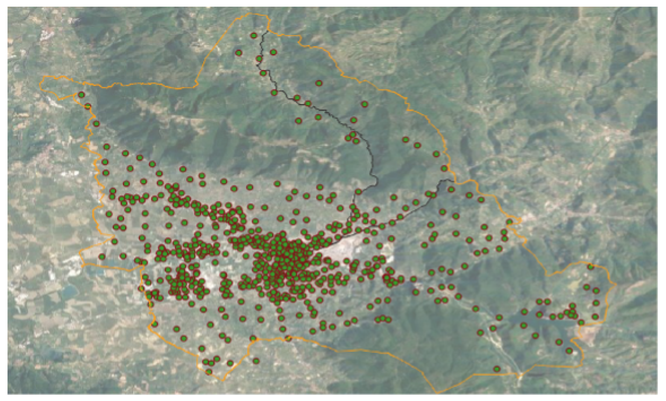
Experimentation data refer to 348 consumers with both energy prediction and flexibility readings over one-hour time intervals retrieved from ASM Terni pilot (https://www.wisegrid.eu/pilot-sites/terni (accessed on 5 May 2021)) in Italy. ASM Terni S.p.A. is an Italian multi-utility, operating in the centre of Italy, notably it is the Distributed System Operator (DSO) of the city of Terni. The local power distribution network expands to a geo-surface of 211 km² and delivers around 400 GWh to 65,500 customers annually. The ASM distribution network connects to the High Voltage (HV) grid through three primary substations and supplies electricity to residential and business customers with 60 Medium Voltage (MV) lines (10 kV to 20 kV) and around 700 secondary substations (Figure 1). The peak power is about 70 MW and the total length of the power lines in the grid is about 2400 km; 600 km MV lines and 1800 km Low Voltage (LV) lines. Currently, the energy customers are about 65,500, 98% of which have an electronic meter. The grid integrates a large number of distributed RES which are connected with the MV and LV distribution networks. These constitute a total installed capacity of about 70 MW (Figure 2). According to this energy mix, half of the GWh (200 out of 400) absorbed yearly, come from DER systems linked with the ASM’s LV/MV grid, while around 70 GWh from intermittent RES.

In 2019 the energy consumption reached 347 GWh, while the distributed production units connected to the MV / LV network (DER) generate 178 GWh (i.e., approximately 49% of the total demand). Therefore, in 2019 about 50% of the total consumption was covered by RES. In fact, in 2019 the local power network received renewable energy from:

• 1325 PV plants, the number of plants connected every year is shown in Figure 3;
• one waste-to-energy;
• eight hydro power plants.

In 2019 the total electric power generated from RES was as follows (energy mix variation is shown in Figure 4):

• 34 GWh from Solar Energy;
• 68 GWh from Hydropower;
• eight GWh from Biomass and waste-to-energy.

For this paper the energy consumption and production of a cluster of 348 consumers have been used for the evaluation purposes. This cluster consists of residential, commercial and industrial end users, characterized by high level of auto-consumption rate. Although almost all the electricity users of the ASM’s power distribution network have smart meters installed in their premises, for many of them monthly values are collected. On the other hand, the data of the cluster are collected every 15 min and aggregated in one-hour resolution for experimentation; these data are gathered through the Advanced Metering Infrastructure (AMI) which consists of a Smart Meter, Current Transformers and GPRS modem that enables data transfer to central servers. After a consistency check data are stored in ASM Terni servers for 5 years.

For further enhancing our dataset, yet another consumer is added to the portfolio of consumers, that is the novel CERTH/ITI nZEB Smart Home (https://smarthome.iti.gr/ (accessed on 11 May 2021)) which is located in Thessaloniki, Greece. It is a rapid prototyping infrastructure incorporating various novel technologies. This structure imitates real domestic conditions experimenting on actual habitat conditions. Since it integrates a variety of Internet of Things (IoT) technologies and Information and Communication Technology (ICT) solutions, it stands as an ideal consumer pilot for this study, presenting its side and its interaction with the aggregator.

The data observations expand from 1 February 2019 up to 27 February 2019. Whenever timeseries are utilized, the timestamp is in coordinated universal time (UTC). System Marginal Price (SMP) is retrieved from the European Network of Transmission System Operators for Electricity (ENTSO-E) transparency platform (https://transparency.entsoe.eu (accessed on 3 April 2021)) for both pilot areas, Italy (348 consumers) and Greece (one consumer). Other important parameters that have been considered are temperature and operating reserves.

The energy load prediction is based on an ensemble of a set of weak learners, such as Multilayer Perceptron (MLP), Long Short-Term Memory (LTSM), Gradient Boosting trees (GBT) and Support Vector Regression (SVR) [22,23]. Their energy forecasting results are combined using a weighted average with the weights being dynamically computed as a function of the input features of the prediction process according to (1):

$${\omega }_{MLP}{*E}_{MLP}+{\omega }_{LTSM}{*E}_{LTSM}+{\omega }_{GBR}{*E}_{GBR}+{\omega }_{SVR}*E_{SVR}$$

(1)

The weights associated with the prediction results of each of the four weak learners (MLP, LSTM, GBT and SVR) are computed using a genetic algorithm. The solution is composed of the four weights and the fitness function is based on the prediction error obtained by applying the weights on the predictions according to the test data. Such an approach is presented in [24], allowing for a dynamic weight computation combined with a weak learner configuration.

The energy demand prediction considers both energy and contextual features. The energy features are determined from the historical energy data acquired by consumers on-site smart meters. The contextual features represent data that are not specific to power but is correlated to context, such as season, day of the week and day of the month. The energy flexibility prediction model uses two MLP neural networks to predict the flexibility lower bound (i.e., below the baseline demand) and upper bound (i.e., above the baseline demand) [24]. The baseline energy demand shows the electricity would have been consumed by a consumer in the absence of DR and to determine it the X of Y method was used. Flexibility prediction features reflect the differences between the monitored energy profiles and the baseline, either above or below. The neurons used are of type ReLU [25], the metric for training the network was MSE [26] and the optimizer used for determining the weights was ADAM [27]. The energy load and flexibility predictions have a good accuracy featuring a MAPE < 10% [26].

Table 1. Dataset description for the two types of optimization.

Optimization Type	Data Description
Consumer	Energy load forecast (kWh);
	System marginal price (€/kWh).
Aggregator	Portfolio load forecast (kWh);
	Portfolio upper bound flexibility of each consumer (kWh);
	Portfolio lower bound flexibility of each consumer (kWh);
	System marginal price (€/kWh).

offers a summary and a description of the data used for experimentation. For bi-objective optimization timeseries data per consumer are utilized. These include energy load forecasts and the SMP. For the single-objective optimization utilize timeseries data for portfolio load forecast are utilized, upper and lower bounds of flexibility and the SMP. A detailed presentation of data and the mathematical problem formation follows in Section 4.2 and Section 4.3.

4.2. Single-Objective Optimization—Aggregator

The optimal day-ahead schedule for the aggregator utilizes lower and upper bounds of flexibility for each consumer within the portfolio and the energy load forecast for a specific day and in one-hour resolution. Since, the aim is to minimize the aggregator’s net cost for trading energy in the day-ahead market, the SMP per market (Italian and Greek) is also considered, exposing capabilities for optimizing overall portfolio economic benefits and the portfolio’s day-ahead energy load forecast based on historical data.

Therefore, this study considers a single-objective modeling approach for minimizing the operational costs for aggregators. Due to the abstract level of input data, a sub-process for testing and validation is exploited utilizing a single objective function for this use case. It yields the “on demand” algorithmic output and the optimal contribution of the consumer to the grid (for a specific timestamp) while abiding with design constraints.

Objective function (2) manages the aggregator’s day-ahead optimal energy resource scheduling, aiming to reduce its overall operational costs and maximize profits.

$$f{a}_{cost}\left(t\right)=min\sum _{i=1}^{N_{tot\_C}}\sum _t^{t_{total}}{E}_{i,imp}\left(t\right)*SMP\left(t\right)*\Delta t$$

(2)

Subject to constraints (3)–(5):

$$E_{i,imp}\left(t\right)\ge fle{x}_{i,lb}\left(t\right)$$

(3)

$$E_{i,imp}\left(t\right)\le fle{x}_{i,ub}\left(t\right)$$

(4)

$$\sum _{i=1}^{N_{tot\_C}}\sum _t^{t_{total}}{E}_{i,imp}\left(t\right)*\Delta t=\sum _{i=1}^{N_{tot\_C}}\sum _t^{t_{total}}{E}_{i,for}\left(t\right)*\Delta t$$

(5)

With constraints (3) and (4), referring to the maximum and minimum amounts of energy that each consumer can reach individually and consequently the portfolio as a whole. Constraint (5) actually states that the sum of the optimized energy scheduling must be equal to that of the initially predicted one. Therefore, taking into account that the overall energy consumption does not change, regardless of the optimized schedule proposed to consumers, their daily consumption habits also do not change.

4.3. Bi-Objective Optimization—Consumer

For optimizing the day-ahead energy scheduling for the consumer, the day-ahead energy load forecast in one-hour resolution is utilized. That way the overall energy load consumption can be retrieved. Using historical data from the said pilots and the knowledge of SMP in both areas, the cost of imported energy for the consumer is calculated.

Bi-objective optimization refers to the consumer use case and the following objectives are considered: operation cost minimization resulting from reducing energy consumption at occupant acceptable levels, and consumer discomfort minimization. These two objective functions are solved simultaneously, considering constraints and common variables.

The objective function related to operation cost reduction is the following:

$$f{p}_{cost}\left(t\right)=min\sum _t^{t_{total}}{E}_{imp}\left(t\right)*EIT\left(t\right)*\Delta t$$

(6)

Subject to constraints (7) and (8):

$$E_{i,imp}\left(t\right)\ge 0,\forall t\in \Delta t$$

(7)

$$E_{i,imp}\left(t\right)\le E_{i,max}*E_{i,for}\left(t\right),\forall t\in \Delta t$$

(8)

Effective energy management involves a certain level of load manipulation for facilities. For households, consumer loads for home appliances are distinguished, which are categorized into fixed, regulatable and deferrable loads. Lightning, cooking and electronic devices belong to the fixed load that should be used anytime, on request. Water heaters and heat, ventilation and air-conditioning (HVAC) systems belong to the regulatable loads, being subjects to usage delay or rescheduling. Appliances, such as dishwashers and dryers, belong to the deferrable loads, since their operation can be deferred. Consumer thermal comfort considering these parameters poses a challenging task for effective and targeted DR scheme implementation [28].

Consumer comfort is subjective and poses significant difficulties for a realistic assessment and quantification. According to ISO7730 thermal comfort standard [29] the Predicted Mean Value (PMV) index is used to calculate human perception of comfort. The PMV index ranges between [−3, 3], where: 0 means neither hot, nor cold; +/−1 slightly warm (+), or slightly cold (−); +/−2 means heat (+), or cold (−); and +/−3 means very hot (+), or very cold (−). Yet, for retrieving PMV index values access to a certain number of data attributes is needed, such as air temperature, air velocity, air humidity, mean radiant temperature, clothing insulation and occupant activity. Since this study has no access to such data, consumer (occupant) discomfort is calculated adjusting a custom index that considers the PMV index value range and discomfort calculation, as presented in [30]. That way, the output of discomfort across all consumers is normalized between values $[0,1]$, distinguishing five discomfort profiles. An example of such profiles is presented in Section 5.1.

The objective function related to the minimization of the consumer discomfort is described as:

$$f{p}_{discomfort\_reduction}\left(t\right)=min\sum _{i=1}^{t_{total}}\frac{C_{preference}}{2}*E_{im{p}_{reduction}}{\left(t\right)}^2+au{x}_{coefficient}*E_{im{p}_{reduction}}$$

(9)

Subject to constraints (7), (8), (10) and (11).

$$C_{preference}>0$$

(10)

$$au{x}_{coefficient}>0$$

(11)

The minimization of consumer discomfort function (9) models the degree of discomfort a consumer feels when reducing the energy consumption. The greater the energy consumption reduction, the greater discomfort [31]. $C_{preference}$ and $au{x}_{coefficient}$ pose as customer-specific variables. A high value of $C_{preference}$ expresses a consumer’s preference to lower energy consumption also decreasing discomfort, while a greater $au{x}_{coefficient}$ value infers to more discomfort [32].

5. Results

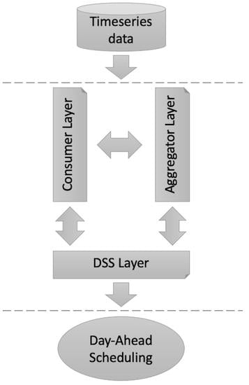
This section presents results as scenarios for the optimization actors. These are, consumers and aggregators. The two optimizations, single- and bi-objective, interact with each other, based on the following architectural scheme forming a tri-layer interaction.

5.1. Scenario #1: Consumer

The Consumer layer optimizes consumer’s energy requirements for one day-ahead, while integrating five personalized options for occupant discomfort. For presentation clarity, the results for a single consumer are presented. The same optimization process, along with its results, applies to all the consumers in the aggregator’s portfolio (as described in Section 4.1).

Figure 5 shows the bi-objective optimization output of the consumer layer for a day-ahead scheduling, along with discomfort options and economic reduction solutions.

The five reduction solutions reflect five distinct levels of discomfort, considered in this work, that is:

• No Optimization (NO): the initially state, prior to any optimization. Serves as a baseline scenario.
• No Discomfort (ND): the case, where the minimum amount of discomfort is considered.
• Slight Discomfort (SD): the case, where a slight level of discomfort is considered.
• Average (AD): the case, where a medium level of discomfort is considered.
• Much Discomfort (MD): the case, where a greater level of discomfort is considered.
• Heavy Discomfort (HD): the case, where the greatest amount of discomfort is considered.

These solutions are presented in Figure 6 in the Pareto front as the outcome of the bi-objective optimization approach. Appendix A (

Table A1. Cost minimization and discomfort options for consumers.

t	No Opt	ND	ND Chg (%)	SD	SD Chg (%)	AD	AD Chg (%)	MD	MD Chg (%)	HD	HD Chg (%)
0	6.418	5.143	−19.866	4.493	−29.994	4.493	−29.994	4.493	−29.994	4.493	−29.994
1	6.347	5.183	−18.339	4.443	−29.998	4.443	−29.998	4.443	−29.998	4.443	−29.998
2	6.356	5.38	−15.356	4.449	−30.003	4.449	−30.003	4.449	−30.003	4.449	−30.003
3	6.386	5.432	−14.939	4.47	−30.003	4.47	−30.003	4.47	−30.003	4.47	−30.003
4	6.309	5.298	−16.025	4.416	−30.005	4.416	−30.005	4.416	−30.005	4.416	−30.005
5	6.276	5.012	−20.140	4.393	−30.003	4.393	−30.003	4.393	−30.003	4.393	−30.003
6	6.409	4.486	−30.005	4.486	−30.005	4.486	−30.005	4.486	−30.005	4.486	−30.005
7	6.951	4.866	−29.996	4.866	−29.996	4.866	−29.996	4.866	−29.996	4.866	−29.996
8	9.763	6.834	−30.001	6.834	−30.001	6.834	−30.001	6.834	−30.001	6.834	−30.001
9	30.334	27.767	−8.462	25.262	−16.721	22.851	−24.669	21.234	−29.999	21.234	−29.999
10	37.325	35.455	−5.010	33.18	−11.105	30.99	−16.973	28.778	−22.899	26.127	−30.001
11	37.855	36.18	−4.425	33.97	−10.263	31.843	−15.882	29.694	−21.559	26.499	−29.999
12	38.13	36.895	−3.239	34.831	−8.652	32.844	−13.863	30.837	−19.127	26.96	−29.295
13	36.906	35.675	−3.336	33.611	−8.928	31.626	−14.307	29.619	−19.745	25.834	−30.001
14	36.11	34.5	−4.459	32.312	−10.518	30.205	−16.353	28.077	−22.246	25.277	−30.000
15	36.691	34.821	−5.097	32.546	−11.297	30.356	−17.266	28.144	−23.295	25.684	−29.999
16	37.139	34.398	−7.380	31.834	−14.284	29.367	−20.927	26.875	−27.637	25.997	−30.001
17	37.803	34.242	−9.420	31.408	−16.917	28.68	−24.133	26.462	−30.000	26.462	−30.000
18	37.065	33.172	−10.503	30.227	−18.449	27.394	−26.092	25.945	−30.001	25.945	−30.001
19	34.999	31.495	−10.012	28.68	−18.055	25.97	−25.798	24.499	−30.001	24.499	−30.001
20	13.621	11.252	−17.392	9.535	−29.998	9.535	−29.998	9.535	−29.998	9.535	−29.998
21	6.819	4.933	−27.658	4.773	−30.004	4.773	−30.004	4.773	−30.004	4.773	−30.004
22	6.673	5.05	−24.322	4.671	−30.001	4.671	−30.001	4.671	−30.001	4.671	−30.001
23	6.593	5.324	−19.248	4.615	−30.002	4.615	−30.002	4.615	−30.002	4.615	−30.002
Total Sum	495.28	448.79	−9.386	414.31	−16.35	388.57	−21.55	366.61	−25.98	346.96	−29.95

) outlines the cost minimization for consumers, based on the five options available. The values presented are for a period of 24 h, expressed in kWh and in relative change form (in %), in terms of the initial value, i.e., No Opt. (NO) Scenario. Figure 5 and Appendix A (Table A1) present results for one day within the examined period of 1 February 2019 up to 27 February 2019, that is, 7 February 2019. Similar results have been produced for every day of the examined period.

5.2. Scenario #2: Aggregator

As in the case of the consumer, cost minimization is the objective, differing only in scale, and constrained by the flexibility of the consumer portfolio, as detailed in Section 4.1. The DSS layer optimization outcome for the aggregator’s consumer portfolio for the day-ahead energy scheduling, can be seen in Figure 7.

The upper and lower flexibility bounds can be seen, as a set for the whole portfolio in black, and the forecasted values in red. The orange dashed line depicts the SMP values, and grey bars show the final optimized per hour energy consumption of the portfolio. The way the actual energy consumption is modified is depicted by the forecasted red line to the grey bars according to the SMP values; whenever the SMP is high, the consumption is lowered to the lowest possible value; whenever the SMP is low, the energy consumption is regained, reaching the highest values possible, in order to have the same total daily energy consumption in the end. According to this scheme, the DR signals to be sent to each of the consumers are calculated. Every time a deviation between the forecasted energy consumption and the optimized one exists, DR signals are to be sent to the consumers. Since the whole DR portfolio is included, the idea is that each consumer should contribute according to his/her capabilities, that is their attributed flexibility, in order to have a fair strategy among them. First, their contribution to the total portfolio flexibility is calculated for every hour as formulated in the following equations:

$$fle{x}_{i,l{b}_{\%}}\left(t\right)=\frac{E_{i,for}\left(t\right)-fle{x}_{i,lb}\left(t\right)}{{\sum }_{i=1}^{N_{tot\_C}}{E}_{i,for}\left(t\right)-{\sum }_{i=1}^{N_{tot\_C}}fle{x}_{i,lb}\left(t\right)}$$

(12)

$$fle{x}_{i,u{b}_{\%}}\left(t\right)=\frac{fle{x}_{i,ub}\left(t\right)-E_{i,for}\left(t\right)}{{\sum }_{i=1}^{N_{tot\_C}}fle{x}_{i,ub}\left(t\right)-{\sum }_{i=1}^{N_{tot\_C}}{E}_{i,for}\left(t\right)}$$

(13)

Then, this is applied to the difference between the optimized and originally forecasted energy consumption for that hour, and the required amount of energy in kWhs to be reduced, or increased, is it may be the case, is calculated for every consumer, as formulated in the following equations, that is:

$$fle{x}_{i,lb}\left(t\right)=\left\{\begin{array}{cc}fle{x}_{i,l{b}_{\%}}\left(t\right)*[\sum _{i=1}^{N_{tot\_C}}{E}_{i,for}\left(t\right)-\sum _{i=1}^{N_{tot\_C}}{E}_{opt}\left(t\right)]\hfill & ,\sum _{i=1}^{N_{tot\_C}}{E}_{i,for}\left(t\right)>\sum _{i=1}^{N_{tot\_C}}{E}_{i,opt}\left(t\right)\hfill \\ 0\hfill & ,\sum _{i=1}^{N_{tot\_C}}{E}_{i,for}\left(t\right)<\sum _{i=1}^{N_{tot\_C}}{E}_{i,opt}\left(t\right)\hfill \end{array}\right.$$

(14)

$$fle{x}_{i,ub}\left(t\right)=\left\{\begin{array}{cc}0\hfill & ,\sum _{i=1}^{N_{tot\_C}}{E}_{i,for}\left(t\right)>\sum _{i=1}^{N_{tot\_C}}{E}_{i,opt}\left(t\right)\hfill \\ fle{x}_{i,u{b}_{\%}}\left(t\right)*[\sum _{i=1}^{N_{tot\_C}}{E}_{i,for}\left(t\right)-\sum _{i=1}^{N_{tot\_C}}{E}_{opt}\left(t\right)]\hfill & ,\sum _{i=1}^{N_{tot\_C}}{E}_{i,for}\left(t\right)<\sum _{i=1}^{N_{tot\_C}}{E}_{i,opt}\left(t\right)\hfill \end{array}\right.$$

(15)

Figure 8 demonstrates an example, highlighting a single optimal solution for part of the portfolio posing as DR signals, e.g., four consumers out of the whole portfolio. Appendix A (

Table A2. Partial one day-ahead portfolio scheduling (10 consumers) with lower (l) and upper (u) bounds of flexibility contribution in kWh.

t	C1 (l, u)	C2 (l, u)	C3 (l, u)	C4 (l, u)	C5 (l, u)	C6 (l, u)	C7 (l, u)	C8 (l, u)	C9 (l, u)	C10 (l, u)
0	(0, 0.46)	(0, 7.86)	(0, 0.32)	(0, 1.79)	(0, 0.57)	(0, 2.04)	(0, 0.49)	(0, 0.37)	(0, 0.76)	(0, 0.62)
1	(0, 0.77)	(0, 4.72)	(0, 0.33)	(0, 0.84)	(0, 0.54)	(0, 1.66)	(0, 0.88)	(0, 0.76)	(0, 0.63)	(0, 0.69)
2	(0, 0.5)	(0, 4.75)	(0, 0.35)	(0, 1.45)	(0, 0.53)	(0, 1.91)	(0, 0.87)	(0, 0.65)	(0, 0.26)	(0, 0.42)
3	(0, 0.58)	(0, 4.15)	(0, 0.43)	(0, 0.82)	(0, 0.42)	(0, 1.05)	(0, 0.49)	(0, 0.4)	(0, 0.3)	(0, 0.72)
4	(0, 0.69)	(0, 4.96)	(0, 0.52)	(0, 1.38)	(0, 0.56)	(0, 0.62)	(0, 1.16)	(0, 0.23)	(0, 0.85)	(0, 0.56)
5	(0, 0.3)	(0, 4.1)	(0, 0.34)	(0, 1.55)	(0, 0.57)	(0, 1.12)	(0, 1.2)	(0, 0.39)	(0, 0.78)	(0, 0.84)
6	(−0.75, 0)	(−4.47, 0)	(−0.33, 0)	(−2.18, 0)	(−0.9, 0)	(−2.53, 0)	(−1.16, 0)	(−0.61, 0)	(−0.61, 0)	(−0.92, 0)
7	(−1.41, 0)	(−4.5, 0)	(−0.37, 0)	(−1.92, 0)	(−1.1, 0)	(−2.26, 0)	(−1.43, 0)	(−0.47, 0)	(−0.58, 0)	(−0.96, 0)
8	(−5.3, 0)	(−5.1, 0)	(−0.34, 0)	(−2.24, 0)	(−1.03, 0)	(−1.75, 0)	(−1.7, 0)	(−1.39, 0)	(−0.85, 0)	(−1.23, 0)
9	(−3.6, 0)	(−4, 0)	(−0.43, 0)	(−1.34, 0)	(−1.42, 0)	(−1.69, 0)	(−1.99, 0)	(−1.24, 0)	(−0.79, 0)	(−0.79, 0)
10	(−4.83, 0)	(−3.16, 0)	(−0.52, 0)	(−6.59, 0)	(−1.1, 0)	(−2.27, 0)	(−1.46, 0)	(−1.56, 0)	(−0.83, 0)	(−1.1, 0)
11	(0, 1.82)	(0, 3.44)	(0, 0.33)	(0, 2.18)	(0, 1.23)	(0, 2.09)	(0, 0.73)	(0, 0.44)	(0, 1)	(0, 0.87)
12	(0, 3.29)	(0, 7.53)	(0, 0.33)	(0, 4.43)	(0, 2.32)	(0, 4.58)	(0, 1.5)	(0, 1.38)	(0, 1.99)	(0, 0.83)
13	(0, 3.71)	(0, 7.43)	(0, 0.39)	(0, 3.71)	(0, 1.85)	(0, 4.8)	(0, 1.19)	(0, 1.78)	(0, 2.5)	(0, 2.24)
14	(0, 5.45)	(0, 9.83)	(0, 0.22)	(0, 5.32)	(0, 1.41)	(0, 4.81)	(0, 1.02)	(0, 0.87)	(0, 2.8)	(0, 0.98)
15	(−2.89, 0)	(−5.95, 0)	(−0.07, 0)	(−4.1, 0)	(−1.14, 0)	(−2.48, 0)	(−0.67, 0)	(−1.41, 0)	(−1.24, 0)	(−1.88, 0)
16	(−3.01, 0)	(−5.87, 0)	(−0.23, 0)	(−2.74, 0)	(−1.38, 0)	(−2.64, 0)	(−0.56, 0)	(−0.96, 0)	(−1.86, 0)	(−1.8, 0)
17	(−3.16, 0)	(−6.04, 0)	(−0.3, 0)	(−3.74, 0)	(−1.06, 0)	(−3.35, 0)	(−0.81, 0)	(−0.58, 0)	(−2.28, 0)	(−1.96, 0)
18	(−3.74, 0)	(−6.1, 0)	(−0.28, 0)	(−3.41, 0)	(−0.53, 0)	(−2.83, 0)	(−0.6, 0)	(−0.7, 0)	(−2.77, 0)	(−1.43, 0)
19	(−0.47, 0)	(−6.66, 0)	(−0.25, 0)	(−2.22, 0)	(−0.41, 0)	(−4.21, 0)	(−0.76, 0)	(−1.51, 0)	(−2.23, 0)	(−0.89, 0)
20	(−0.58, 0)	(−8.46, 0)	(−0.28, 0)	(−2.03, 0)	(−0.64, 0)	(−3.9, 0)	(−0.62, 0)	(−1.56, 0)	(−1.57, 0)	(−0.63, 0)
21	(−0.5, 0)	(−9.41, 0)	(−0.21, 0)	(−3.56, 0)	(−0.43, 0)	(−3.79, 0)	(−0.34, 0)	(−0.9, 0)	(−1.57, 0)	(−0.41, 0)
22	(0, 0.88)	(0, 10.64)	(0, 0.3)	(0, 4.36)	(0, 0.5)	(0, 3)	(0, 0.95)	(0, 1.31)	(0, 2.2)	(0, 0.4)
23	(0, 0.88)	(0, 7.79)	(0, 0.43)	(0, 4.89)	(0, 0.46)	(0, 4.11)	(0, 0.98)	(0, 0.47)	(0, 1.58)	(0, 0.54)

) offers a more detailed representation, each column presenting a consumer and each row showing the lowest and upper bounds of flexibility contribution per timestamp. These values stand for the individualized deviations (per consumer) from the Portfolio Forecasted Consumption depicted in Figure 7. The aforementioned results for the same day period are presented, as those in Figure 5 and Figure 7.

Finally, in

Table 2. Portfolio savings for a week (1 February 2019 up to 7 February 2019).

Timestamp	Portfolio Initial Cost (€)	Optimization Savings (€)	Final Cost (€)	Cost Savings (%)
1 February 2019	6282.314	441.9311	5840.3829	−7.0345
2 February 2019	4799.9383	315.214	4484.7243	−6.567
3 February 2019	4393.4721	332.1233	4061.3488	−7.5594
4 February 2019	6114.7628	498.09	5616.6728	−8.1456
5 February 2019	5715.1828	235.5469	5479.6359	−4.1214
6 February 2019	5424.4863	351.2224	5073.2639	−6.4747
7 February 2019 *	5892.0956	344.1329	5547.9627	−5.8406

* This timestamp relates to portfolio savings resulting from optimization output presented in Figure 7.

a representative sample of portfolio savings for the whole examined period between 1 February 2019 up to 7 February 2019 is presented.

5.3. Proposed Demand Response Scheme

The proposed DR scheme envisions an autonomous and dynamic improvement for optimal energy management involving two or more actors. At its current form, it utilizes the optimization outputs for consumer and aggregator attempting to enhance their collaboration while pertaining certain levels of freedom of choice for managing assets. Both the consumer and the aggregator may choose their own optimized schedules, according to the electricity price and in parallel. The conception of such a DR scheme generates new capabilities for energy contract relaxation, while allowing optimization on the P2P level. More specifically, since day-ahead energy load scheduling is considered, the aggregator publishes an hourly DR schedule for all portfolio assets, i.e., consumers, at a fixed timestamp the day before. For the examined use cases, this means on 6 February 2019 at 18:00, since in most markets the SMP for the day-ahead is determined around noon on the previous day. Then, the consumers have to accept the DR signals and a two-hour period is provided for them to respond, that is, 19.00–21.00. The decision of whether to accept or reject the DR signals received, is based mainly on their alignment with the optimized day-ahead schedule already selected by each consumer. Thus, some DR signals may only be rejected, while others may be either Accepted or Rejected. This scheme is implemented by the DSS layer and generates default options for the involved actors (Figure 9).

Next, three use cases of the proposed DR Scheme are presented for a single consumer (C1), considering the results from Appendix A (Table A1 and Table A2).

Table 3. Envisioned DR scheme and interaction between consumer and aggregator. No optimization for consumer.

t	Energy Load Forecast (No Opt)	DRS (C1)	Requested Energy Load (C1)	Status
0	6.418	0.46	6.878	Reject
1	6.347	0.77	7.117	Reject
2	6.356	0.5	6.856	Reject
3	6.386	0.58	6.966	Reject
4	6.309	0.69	6.999	Reject
5	6.276	0.3	6.576	Reject
6	6.409	−0.75	5.659	Accept/Reject
7	6.951	−1.41	5.541	Accept/Reject
8	9.763	−5.3	4.463	Accept/Reject
9	30.334	−3.6	26.734	Accept/Reject
10	37.325	−4.83	32.495	Accept/Reject
11	37.855	1.82	39.675	Reject
12	38.13	3.29	41.420	Reject
13	36.906	3.71	40.616	Reject
14	36.11	5.45	41.560	Reject
15	36.691	−2.89	33.801	Accept/Reject
16	37.139	−3.01	34.129	Accept/Reject
17	37.803	−3.16	34.643	Accept/Reject
18	37.065	−3.74	33.325	Accept/Reject
19	34.999	−0.47	34.529	Accept/Reject
20	13.621	−0.58	13.041	Accept/Reject
21	6.819	−0.5	6.319	Accept/Reject
22	6.673	0.88	7.553	Reject
23	6.593	0.88	7.473	Reject

,

Table 4. Envisioned DR scheme and interaction between consumer and aggregator. Slight Discomfort (SD) for consumer.

t	Max Energy Load (No Opt)	Min Energy Load (SD)	DRS (C1)	Requested Energy Load (C1)	Status
0	6.418	4.493	0.46	4.953	Accept/Reject
1	6.347	4.443	0.77	5.213	Accept/Reject
2	6.356	4.449	0.5	4.949	Accept/Reject
3	6.386	4.47	0.58	5.050	Accept/Reject
4	6.309	4.416	0.69	5.106	Accept/Reject
5	6.276	4.393	0.3	4.693	Accept/Reject
6	6.409	4.486	−0.75	3.736	Accept/Reject
7	6.951	4.866	−1.41	3.456	Accept/Reject
8	9.763	6.834	−5.3	1.534	Accept/Reject
9	30.334	25.262	−3.6	21.662	Accept/Reject
10	37.325	33.18	−4.83	28.350	Accept/Reject
11	37.855	33.97	1.82	35.790	Accept/Reject
12	38.13	34.831	3.29	38.121	Accept/Reject
13	36.906	33.611	3.71	37.321	Reject
14	36.11	32.312	5.45	37.762	Reject
15	36.691	32.546	−2.89	29.656	Accept/Reject
16	37.139	31.834	−3.01	28.824	Accept/Reject
17	37.803	31.408	−3.16	28.248	Accept/Reject
18	37.065	30.227	−3.74	26.487	Accept/Reject
19	34.999	28.68	−0.47	28.210	Accept/Reject
20	13.621	9.535	−0.58	8.955	Accept/Reject
21	6.819	4.773	−0.5	4.273	Accept/Reject
22	6.673	4.671	0.88	5.551	Accept/Reject
23	6.593	4.615	0.88	5.495	Accept/Reject

and

Table 5. Envisioned DR scheme and interaction between consumer and aggregator. Heavy Discomfort (HD) for consumer.

t	Max Energy Load (No Opt)	Min Energy Load (HD)	DRS (C1)	Requested Energy Load (C1)	Status
0	6.418	4.493	0.46	4.953	Accept/Reject
1	6.347	4.443	0.77	5.213	Accept/Reject
2	6.356	4.449	0.5	4.949	Accept/Reject
3	6.386	4.47	0.58	5.050	Accept/Reject
4	6.309	4.416	0.69	5.106	Accept/Reject
5	6.276	4.393	0.3	4.693	Accept/Reject
6	6.409	4.486	−0.75	3.736	Accept/Reject
7	6.951	4.866	−1.41	3.456	Accept/Reject
8	9.763	6.834	−5.3	1.534	Accept/Reject
9	30.334	21.234	−3.6	17.634	Accept/Reject
10	37.325	26.127	−4.83	21.297	Accept/Reject
11	37.855	26.499	1.82	28.319	Accept/Reject
12	38.13	26.96	3.29	30.250	Accept/Reject
13	36.906	25.834	3.71	29.544	Accept/Reject
14	36.11	25.277	5.45	30.727	Accept/Reject
15	36.691	25.684	−2.89	22.794	Accept/Reject
16	37.139	25.997	−3.01	22.987	Accept/Reject
17	37.803	26.462	−3.16	23.302	Accept/Reject
18	37.065	25.945	−3.74	22.205	Accept/Reject
19	34.999	24.499	−0.47	24.029	Accept/Reject
20	13.621	9.535	−0.58	8.955	Accept/Reject
21	6.819	4.773	−0.5	4.273	Accept/Reject
22	6.673	4.671	0.88	5.551	Accept/Reject
23	6.593	4.615	0.88	5.495	Accept/Reject

, show the envisioned DR scheme functionality for consumer (No Opt, SD and HD) to aggregator interaction, allowing consumers to choose which DR signals to accept, or decline. This type of interaction allows a more dynamic adjustment of the energy load while retaining certain levels of discomfort or economical benefits.

6. Conclusions

This study envisions a DSS framework that optimizes day-ahead energy scheduling for aggregators and consumers. The goal is to produce material for academic and industrial reference, focusing on the concepts of multi-objective optimization, applied to demand-side management material, such as DR, flexibility, energy load forecasting and discomfort. An optimization architectural layer describes and solves an individualized problem for each actor, while actor interaction is managed by a third architectural DSS layer. The importance of effective energy management is highlighted and the benefits it yields, while envisioning a cooperative energy management between the aggregator and the consumer. Any improvements in this type of cooperation, generates new prospects for efficient energy monitoring and management for modern energy systems.

For presenting and validating findings, two distinct scenarios have been considered, one referring to consumer optimization and one to aggregator portfolio optimization. The first scenario models cost minimization offering acceptable options without violating the comfort of consumers, and addresses the problem with a large-scale nonlinear solver. The second scenario enables portfolio cost minimization for aggregators, and solves the problem using mixed integer linear programming. Both problem solutions utilize a common framework for communicating the results envisioning a DR scheme that improves prospects for their collaboration. An inclusive collaborative schema has been implemented enabling both the aggregator and the consumer to engage in DR events, yet retaining their autonomy, especially for the consumer, following a human-centric approach towards the end-user, who is the consumer. The results show significant gains in cost savings for both the aggregator and the consumer.

6.1. Limitations

The limitations of this optimization framework can be attributed to the fact that this research does not consider constraints, such as power transmission loss, heating losses, inventors and distances for calculating the objectives. That is because the final product of energy load forecast, flexibility, etc., it retrieved from API pilots. Therefore, this detail is already taken into consideration and pre-calculated, rendering our research design into a high-level experimental approach.

This study aims to optimize one day-ahead energy scheduling, incorporating a DR scheme and two system stakeholders: the consumer and the aggregator. For a more holistic approach, a framework that includes DSO as the third system stakeholder should be contemplated and elaborated on, experimenting on their possible interactions in different scenarios.

An analytical comparative analysis regarding the options of solvers for producing optimization results for each scenario is omitted, since it is considered out of our current research objectives. A large-scale nonlinear optimization and a mixed integer programming solver are utilized to outputting results for consumer and aggregator respectively. Metaheuristics involving genetic algorithms could be incorporated for both scenarios while offering a thorough comparative analysis on solvers. Such limitations generate directions for improvements and future work.

6.2. Implications

This study aims to produce a framework able to optimize the day-ahead energy load scheduling as a holistic approach, taking into account both the aggregator’s and the consumer’s view. Currently, it considers a DR scheme that manages the interaction of two stakeholders (aggregator and consumer). In its expanded version, it should be able to handle also the DSO and validate a three-stakeholder interaction through various use cases. In that case, the framework will be able to identify, test and evaluate a wider range of requirements for a modern energy distribution network. The proposed framework models and offers insights for optimal energy management, acknowledging the possible integratiofn among a variety of parameters, such as RES, and storage units. Integration of such parameters may offer enhanced energy grid elasticity, since there are more options for handling issues related with peak loads, broken power grid links, etc. Such parameters have been identified and presented in the literature, and can be added to an extended version of this work adjusting the objective functions per stakeholder.

Solving each problem in a stand-alone manner allows interactions between consumers (P2P level) while allowing DSO to validate DR programs for the aggregator. Constraints and constants are combined for each case affecting individualized solutions. Novel solutions for a more efficient monitoring and management of energy grid are important. Nowadays, aggregators have to manage hundreds of thousands of consumers constituting very large portfolios showcasing the importance for more efficient energy load scheduling. DSOs also need reliable tools for monitoring, validating and enforcing a constant and reliable energy grid functionality, when deemed necessary. In detail, aggregators should be able to efficiently broadcast a one day-ahead energy load schedule for their portfolios, based on SMP, flexibility setpoints for consumers and more. The consumers require 24/7 asset management and an efficient framework that enables a reliable DR signal confirmation scheme, ideally with dynamic participation. The DSO should retrieve that information from the aggregator and approve the DR portfolio schedule. In case of an energy grid issue, DSO should be able to identify the problem with the power distribution network and notify the aggregator in order to comply with the adjusted one day-ahead energy load and flexibility requests.

In that respect, this work will be able to assist or become a point of reference for both the industry and academia, when referring to DERs, P2P energy transfer models and multi-objective optimization on distribution of energy, considering multi energy assets and actors within an energy ecosystem.

6.3. Future Work

The proposed framework conceptualizes a DSS tool for energy stakeholders based on an optimization engine. It envisions multi-level, multi-factor and multi-objective problem modeling for solving practical problems in the energy sector. The aim is to improve this study according to the following points.

• Continue monitoring the evolution of research on multi-objective optimization in the energy sector. Enforce improvements to the proposed methodology by tackling limitations, as explained in Section 6.1 and by enhancing the perception on objective functions.
• Improve the proposed framework by further automating the methodology in a way that it can act as stand-alone software, which can be utilized given just the appropriate input datasets.
• Add one more architectural layer, the DSO layer, leading to a tri-level optimization approach. The DSO layer is to be conceived as tri-objective optimization problem, considering three objective functions simultaneously. Minimization of grid energy losses, voltage profile improvement and cost reduction of environmental emissions.
• Implement the proposed DR scheme in a more sophisticated way, including technologies, such as Blockchain [33]. This would enhance the business perspective of the proposed framework, while addressing more practical applications of this study.

References

- Jahn, J. Scalarization in multi objective optimization. In Mathematics of Multi Objective Optimization; Springer: Vienna, Austria, 1985; pp. 45–88. [Google Scholar]
- Poli, R.; Koza, J. Genetic programming. In Search Methodologies; Springer: Boston, MA, USA, 2014; pp. 143–185. [Google Scholar]
- Koukaras, P.; Tjortjis, C.; Gkaidatzis, P.; Bezas, N.; Ioannidis, D.; Tzovaras, D. An interdisciplinary approach on efficient virtual microgrid to virtual microgrid energy balancing incorporating data preprocessing techniques. Computing 2021, 1–42. [Google Scholar] [CrossRef]
- Cui, Y.; Geng, Z.; Zhu, Q.; Han, Y. Multi-objective optimization methods and application in energy saving. Energy 2017, 125, 681–704. [Google Scholar] [CrossRef]
- Ren, H.; Zhou, W.; Nakagami, K.; Gao, W.; Wu, Q. Multi-objective optimization for the operation of distributed energy systems considering economic and environmental aspects. Appl. Energy 2010, 87, 3642–3651. [Google Scholar] [CrossRef]
- Lu, Y.; Wang, S.; Zhao, Y.; Yan, C. Renewable energy system optimization of low/zero energy buildings using single-objective and multi-objective optimization methods. Energy Build. 2015, 89, 61–75. [Google Scholar] [CrossRef]
- Karmellos, M.; Mavrotas, G. Multi-objective optimization and comparison framework for the design of Distributed Energy Systems. Energy Convers. Manag. 2019, 180, 473–495. [Google Scholar] [CrossRef]
- Yang, R.; Wang, L. Multi-objective optimization for decision-making of energy and comfort management in building automation and control. Sustain. Cities Soc. 2012, 2, 1–7. [Google Scholar] [CrossRef]
- Marino, C.; Quddus, M.A.; Marufuzzaman, M.; Cowan, M.; Bednar, A.E. A chance-constrained two-stage stochastic programming model for reliable microgrid operations under power demand uncertainty. Sustain. Energy Grids Netw. 2018, 13, 66–77. [Google Scholar] [CrossRef]
- Sefidgar-Dezfouli, A.; Joorabian, M.; Mashhour, E. A multiple chance-constrained model for optimal scheduling of microgrids considering normal and emergency operation. Int. J. Electr. Power Energy Syst. 2019, 112, 370–380. [Google Scholar] [CrossRef]
- Ciftci, O.; Mehrtash, M.; Safdarian, F.; Kargarian, A. Chance-constrained microgrid energy management with flexibility constraints provided by battery storage. In Proceedings of the 2019 IEEE Texas Power and Energy Conference (TPEC), College Station, TX, USA, 7–8 February 2019; pp. 1–6. [Google Scholar]
- Zare, M.; Niknam, T.; Azizipanah-Abarghooee, R.; Ostadi, A. New stochastic bi-objective optimal cost and chance of operation management approach for smart microgrid. IEEE Trans. Ind. Inform. 2016, 12, 2031–2040. [Google Scholar] [CrossRef]
- Nojavan, S.; Majidi, M.; Najafi-Ghalelou, A.; Ghahramani, M.; Zare, K. A cost-emission model for fuel cell/PV/battery hybrid energy system in the presence of demand response program: ε-constraint method and fuzzy satisfying approach. Energy Convers. Manag. 2017, 138, 383–392. [Google Scholar] [CrossRef]
- Yang, S.; Tan, Z.; Liu, Z.; Lin, H.; Ju, L.; Zhou, F.; Li, J. A multi-objective stochastic optimization model for electricity retailers with energy storage system considering uncertainty and demand response. J. Clean. Prod. 2020, 277, 124017. [Google Scholar] [CrossRef]
- Park, M.; Lee, J.; Won, D.J. Demand Response Strategy of Energy Prosumer Based on Robust Optimization Through Aggregator. IEEE Access 2020, 8, 202969–202979. [Google Scholar] [CrossRef]
- Menniti, D.; Pinnarelli, A.; Sorrentino, N.; Burgio, A.; Brusco, G. Demand response program implementation in an energy district of domestic prosumers. In Proceedings of the 2013 Africon, Mauritius, 9–12 September 2013; pp. 1–7. [Google Scholar] [CrossRef]
- Daneshvar, M.; Mohammadi-Ivatloo, B.; Asadi, S.; Anvari-Moghaddam, A.; Rasouli, M.; Abapour, M.; Gharehpetian, B.G. Chance-constrained models for transactive energy management of interconnected microgrid clusters. J. Clean. Prod. 2020, 271, 122177. [Google Scholar] [CrossRef]
- Palli, N.; McCluskey, P.; Azarm, S.; Sundararajan, R. An interactive multistage ε-inequality constraint method for multiple objectives decision making. In Proceedings of the International Design Engineering Technical Conferences and Computers and Information in Engineering Conference, Atlanta, GA, USA, 13–16 September 1998; American Society of Mechanical Engineers: Atlanta, GA, USA, 1998; Volume 80326, p. V002T02A006. [Google Scholar]
- Alvarez-Benitez, J.E.; Everson, R.M.; Fieldsend, J.E. A MOPSO algorithm based exclusively on pareto dominance concepts. In Proceedings of the International Conference on Evolutionary Multi-Criterion Optimization, Guanajuato, Mexico, 9–11 March 2005; Springer: Berlin/Heidelberg, Germany, 2005; pp. 459–473. [Google Scholar]
- Yuan, Y.; Xu, H.; Wang, B. An improved NSGA-III procedure for evolutionary many-objective optimization. In Proceedings of the 2014 Annual Conference on Genetic and Evolutionary Computation, Vancouver, BC, Canada, 12–16 July 2014; pp. 661–668. [Google Scholar]
- Kim, M.; Hiroyasu, T.; Miki, M.; Watanabe, S. SPEA2+: Improving the performance of the strength Pareto evolutionary algorithm 2. In Proceedings of the International Conference on Parallel Problem Solving from Nature, Birmingham, UK, 18–22 September 2004; Springer: Berlin/Heidelberg, Germany, 2004; pp. 742–751. [Google Scholar]
- Ves, A.V.; Ghitescu, N.; Pop, C.; Antal, M.; Cioara, T.; Anghel, I.; Salomie, I. A Stacking Multi-Learning Ensemble Model for Predicting Near Real Time Energy Consumption Demand of Residential Buildings. In Proceedings of the 2019 IEEE 15th International Conference on Intelligent Computer Communication and Processing (ICCP), Cluj-Napoca, Romania, 5–7 September 2019; pp. 183–189. [Google Scholar]
- Petrican, T.; Vesa, A.V.; Antal, M.; Pop, C.; Cioara, T.; Anghel, I.; Salomie, I. Evaluating forecasting techniques for integrating household energy prosumers into smart grids. In Proceedings of the 2018 IEEE 14th International Conference on Intelligent Computer Communication and Processing (ICCP), Cluj-Napoca, Romania, 6–8 September 2018; pp. 79–85. [Google Scholar]
- Vesa, A.V.; Cioara, T.; Anghel, I.; Antal, M.; Pop, C.; Iancu, B.; Salomie, I.; Dadarlat, V.T. Energy flexibility prediction for data center engagement in demand response programs. Sustainability 2020, 12, 1417. [Google Scholar] [CrossRef] [Green Version]
- Nair, V.; Hinton, G.E. Rectified linear units improve restricted boltzmann machines. In Proceedings of the ICML 2010, Haifa, Israel, 21–24 June 2010. [Google Scholar]
- Botchkarev, A. Performance metrics (error measures) in machine learning regression, forecasting and prognostics: Properties and typology. arXiv 2018, arXiv:1809.03006. [Google Scholar]
- Kingma, D.P.; Ba, J. Adam: A method for stochastic optimization. arXiv 2014, arXiv:1412.6980. [Google Scholar]
- Zhang, D.; Li, S.; Sun, M.; O’Neill, Z. An optimal and learning-based demand response and home energy management system. IEEE Trans. Smart Grid 2016, 7, 1790–1801. [Google Scholar] [CrossRef]
- Standardization ISO. ISO 7730 2005-11-15 Ergonomics of the Thermal Environment: Analytical Determination and Interpretation of Thermal Comfort Using Calculation of the PMV and PPD Indices and Local Thermal Comfort Criteria; International Standards, ISO: Geneva, Switzerland, 2005. [Google Scholar]
- Lu, R.; Hong, S.H. Incentive-based demand response for smart grid with reinforcement learning and deep neural network. Appl. Energy 2019, 236, 937–949. [Google Scholar] [CrossRef]
- Yu, M.; Lu, R.; Hong, S.H. A real-time decision model for industrial load management in a smart grid. Appl. Energy 2016, 183, 1488–1497. [Google Scholar] [CrossRef]
- Yu, M.; Hong, S.H. Incentive-Based demand response considering hierarchical electricity market: A Stackelberg game approach. Appl. Energy 2017, 203, 267–279. [Google Scholar] [CrossRef]
- Tsolakis, A.C.; Moschos, I.; Votis, K.; Ioannidis, D.; Dimitrios, T.; Pandey, P.; Katsikas, S.; Kotsakis, E.; García-Castro, R. A Secured and Trusted Demand Response system based on Blockchain technologies. In Proceedings of the 2018 Innovations in Intelligent Systems and Applications (INISTA), Thessaloniki, Greece, 3–5 July 2018; pp. 1–6. [Google Scholar]