Abstract
The growing share of renewable energies in power production and the rise of the market share of battery electric vehicles increase the demand for battery technologies. In both fields, a predictable operation requires knowledge of the internal battery state, especially its state of charge (SoC). Since a direct measurement of the SoC is not possible, Kalman filter-based estimation methods are widely used. In this work, a step-by-step guide for the implementation and tuning of an extended Kalman filter (EKF) is presented. The structured approach of this paper reduces efforts compared with empirical filter tuning and can be adapted to various battery models, systems, and cell types. This work can act as a tutorial describing all steps to get a working SoC estimator based on an extended Kalman filter.
1. Introduction
Lithium-ion batteries (LIB) have shown great potential as an energy storage technology for electrified transportation, portable electronics, and grid stabilization. In contrast to a fuel tank, the remaining energy in a battery cannot be measured directly. Therefore, the internal state of a battery has to be derived from accessible measurement values using mathematical models. These include physical models, data-driven models using machine learning, and equivalent circuit models (ECM). Physical models use differential equations to describe the electrochemical processes inside the cell. These are complex and require detailed information about the cells’ composition for accurate parameterization, but provide a detailed description of the processes inside a cell during a wide range of operating conditions [1]. In data-driven models, machine learning algorithms are used to derive the model directly from measured data without prior knowledge of the cell. However, machine learning algorithms require large data sets to properly train the model [2]. Equivalent circuit models (ECM) describe the batteries’ behaviour using voltage sources and passive electrical components, typically resistors and capacitors. The model parameters are determined by fitting the model prediction to measured responses. Compared with physical models, they do not provide detailed insight in internal processes, but are less complex and therefore easier to parameterize. ECMs provide a good compromise between accuracy and complexity, and are therefore used in many applications [1,3,4,5,6,7,8,9,10,11,12,13,14,15]. Models are always a simplification of reality. Model parameters are imprecise, and sensor measurements are noisy. As a result, the prediction of the model diverges from the true system response. To reduce the prediction error, several mathematical filtering techniques have been introduced [16]. A common approach used in LIB applications is the extended Kalman Filter (EKF) [3,9]. It is widely used to estimate the state of charge [17,18], state of health [1], and cell capacity [6,19]. It can also be used for online parameter estimation [20]. A major challenge is the adjustment of the EKF to the specific application. An improperly tuned filter can lead to unstable and unpredictable behavior [21]. In contrast to other publications [7,10,11,12] which tune the filter empirically, this paper systematically determines the required settings. In this process, a novel extension for handling current sensor noise is proposed. As an additional improvement, this work extends the common battery model by a hysteresis element, which is often omitted in the literature [7,10,11,12,13,14,15,21]. Battery systems often consist of many cells. The SoC estimation on a system level is always based on estimating the SoC of single cells [22]. Therefore, this paper focuses on single-cell SoC estimation only.
Structure of the Paper
Section 2 describes the theory of the battery model and the extended Kalman filter (EKF). In Section 3, EKF extensions for determining the process noise matrix, handling current sensor noise, and filter initialization are introduced. In Section 4, methods for cell characterization are introduced. Section 5 provides a step-by-step guide for setting up the EKF for application. Finally, Section 6 shows an experimental validation.
2. Theory
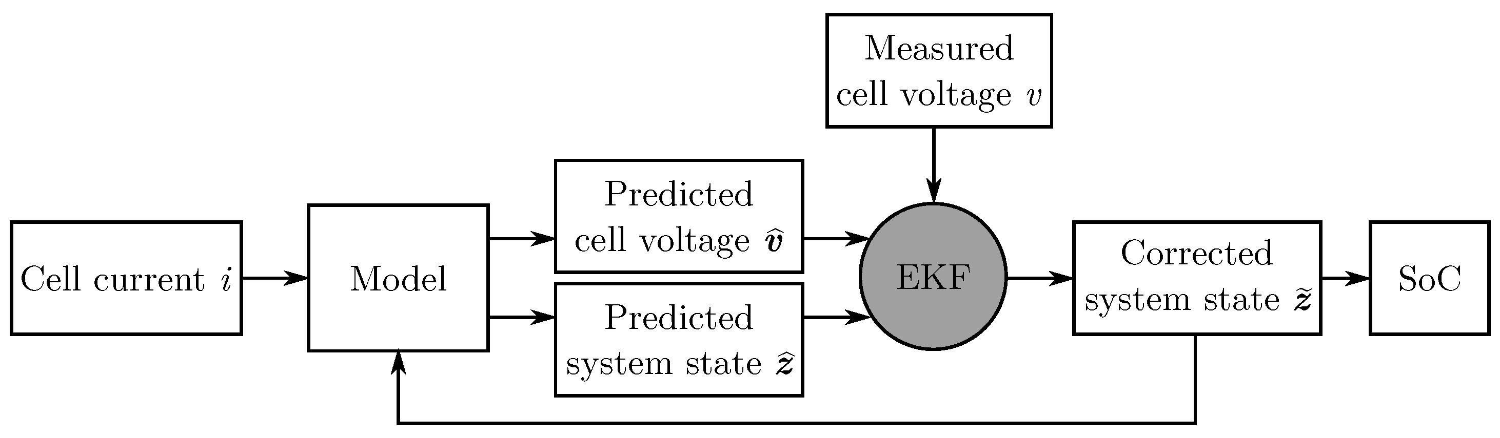
The principle of the extended Kalman filter for SoC estimation is shown in Figure 1. The EKF compares the measured cell voltage and the cell voltage predicted by a battery model. The model also predicts internal, immeasurable states. One of these states is the SoC of the battery cell. In a second step, the EKF corrects the internal states under consideration of the estimated accuracies of the measurement and the model prediction. Thus, it provides a corrected estimation of the SoC.
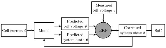
Figure 1.
Principle of an EKF for battery SoC estimation.
2.1. Battery Model
The proposed Kalman filter is based on an equivalent circuit model (ECM) to describe the cells’ behavior. Compared to other models, such as physical models, ECMs offer low computational complexity, require a small amount of parameters, and still provide good approximation [1,9]. Therefore, they are widely used in battery modeling applications [1,3,4,5,6,7,8,9,10,11,12,13,14,15]. Figure 2 shows the ECM proposed here. The associated equations are (1) to (6). A detailed explanation of the model is given by [1].
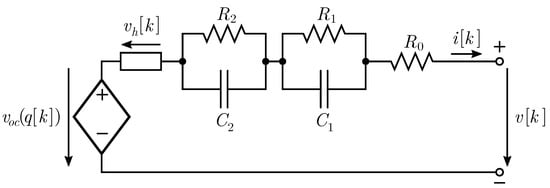
Figure 2.
Equivalent circuit model with two RC elements and hysteresis similar to [1].
The sign of the current is positive for discharging and negative for charging processes.
Note that unlike [1], this paper uses the charge q instead of the state of charge , which makes Equation (2) independent of the cell capacity .
In contrast to many other approaches [7,10,11,12,13,14,15], the used model includes a hysteresis element, as proposed in [1]. The importance of this additional element is supported by the measurement of charging and discharging OCV curves, as described later. The effect of an instantaneous hysteresis as mentioned in [1] is not considered here.
2.2. Extended Kalman Filter for Battery SoC Estimation
The proposed model is nonlinear. In particular, the hysteresis voltage does not depend linearly on the current i. is also non-linear. This is why the original Kalman filter [23] cannot be used here. The extended Kalman filter (EKF) can handle these nonlinear dependencies [9]. The standard algorithm of the EKF is shown in Table 1. Here, predicted quantities are labeled with a hat (), and corrected variables with a tilde (). and are input and output values, and therefore are not labeled.

Table 1.
Standard system and algorithm description of the extended Kalman filter.
For applying the EKF to SoC estimation, the general system description of the EKF is compared with the battery model and equivalents are identified. The comparison in Table 2 demonstrates this process.
Table 2.
Comparison of the general description of the EKF and the used equivalent circuit model of a battery cell.
After the identification of these equivalents, the matrices needed for the EKF algorithm can be derived. For a shorter notation, the following expressions are defined:
The measurement noise matrix is found as the precision of the voltage measurement:
The determination of the process noise matrix , which is defined as is a harder task. A possible approach is presented in Section 3.1.
3. Useful Extensions to the EKF Algorithm
For a well-performing EKF, the tuning and initialization of the filter is critical [21,24]. The relevant matrices for tuning are the measurement noise and the process noise . For the initialization, the initial state and its error have to be set [21].
The determination of is already presented in Equation (11). However, the standard EKF algorithm presents no method for the derivation of the remaining variables and and .
The following extensions give methodic approaches for the tuning and initialization of the EKF. In Section 3.1 and Section 3.2, the matrix is derived from the errors of the model parameters and the noise of the current measurement. The setting of and is described in Section 3.3 in detail.
3.1. Determination of the Process Noise from Parameter Errors
No model fits reality perfectly. The process noise matrix quantizes the inaccuracies in the state equation of the given model. The origins of these inaccuracies are improper parameter values or the structure of the model [24].
In other words, the matrix indicates how precisely the state can be predicted when the state is known. Hence, is added to the system state error at each time step (see Table 1). significantly impacts the strength of the EKF’s correction of the state prediction.
An appropriate choice of the process noise matrix is a difficult but important task [24]. The authors of [24] remark that is often not systematically determined in EKF designs. In many implementations of an EKF for SoC estimation [7,10,11,12], this matrix is established experimentally.
However, an empirical choice of the design matrices cannot guarantee a working filter and cannot be generalized for other models. Therefore, this paper describes how to systematically derive based on the method described in [24].
According to [24], the matrix can be derived from the covariance of the parameters in the model. For the mathematical description, the parameters are summarized in a vector which is
for the model used here. The associated covariance matrix is called . Then, the process noise covariance is obtained as
where
Applying this definition of to the model used here results in the matrix shown in Equation (15).
with
Since can change at every iteration, depending on the current and the system state, the matrix can also change. The notation is therefore necessary.
A variable matrix is more sensible than a constant, as used in [7,10,11,12]. Now the Kalman filter knows that the state of the system is known more precisely in certain situations. For example, if , most of the entries in disappear. This is reasonable: If no current flows, is exactly zero, without any uncertainty. The hysteresis voltage is unchanged . The model uncertainty of each RC voltage decreases in time as the voltage itself decreases. This behavior is only represented by an adaptive matrix.
Finally, for the calculation of the process noise matrix , just the parameter covariances are required. The parameters are assumed to be uncorrelated. The standard deviation or uncertainty of a parameter x is denoted by , the variance . The parameters are assumed to be uncorrelated. Then the parameter covariance matrix is obtained as
3.2. Current Error Contribution to the Process Noise
Another source of error in the prediction of from is the current. In the real battery system, the current is gained by a noisy measurement. The error of this measurement is one of the reasons why simple Coulomb-counting SoC estimators have poor long-term accuracy [9].
There exists no covariance matrix for the input variable in the theoretical description of the EKF like the matrix for the measurement variable. Instead, the matrix is meant to contain all uncertainties of the system equation, including input errors implicitly.
For the systematical derivation of the matrix, the current error has to be included computationally. For this purpose, [25] propose a method for linear Kalman filtering with noisy input variables. A similar derivation can be performed for the extended Kalman filter. Its idea is analogue to the considerations of [24] regarding the derivation of the matrix from parameter errors, and is presented in the following.
Let be the noise of and the associated covariance matrix. Then, the state equation is denoted as
By Taylor series expansion and omission of higher-order terms, the state equation can be rewritten as
This results in the following calculation of the matrix:
where is the process noise without input (or current) error consideration. Using a current sensor with precision (the precision can depend on the current in general), the matrix is
for the proposed battery model and the definition of the input variable vector . The process noise is finally calculated as
For a better understanding, the entry is regarded, which gives the uncertainty of the prediction of the charge q:
For , the Kalman filter could not significantly correct the charge q predicted by Equation (2) and hence produce almost the same result as a Coulomb counter. By the proposed matrix, the current error determines how freely the Kalman filter can deviate from the Coulomb-counting prediction.
In [21] the authors propose a similar derivation of from the current error. In contrast to this work, they assume perfect models with no parameter errors, and therefore do not regard the first part of the matrix calculation according to Section 3.1.
3.3. Initialisation
For the initialisation of the EKF algorithm, the system state and its error have to be estimated. The initial state might be well-known under certain conditions, whereas the error of the initial state is quite hard to guess.
It is useful to start the EKF in a defined state, for example after a long resting time. Then the best estimation for the initial state is
where is chosen such that .
For an estimation of the initial state error , a method described in [24] can be applied. This method is also used in [21]. The Ref. [24] supposes to estimate an upper limit and a lower limit for the initial system state and calculate the initial state error as
The limits , and will be established in the following equations. Hereby, it is assumed that and the system was in rest for before the initialization.
The only state that can be determined precisely is due to . That means the upper and lower limits for this state are 0.
In general, the RC elements are not completely discharged at initialization, resulting in an error on the estimation . Let be the maximum allowed absolute value for currents in the system. Then the limits for the initial RC voltages are
Independent of the current, the hysteresis voltage varies between M and , so that the limits can be estimated as
The most difficult state is q, since it is obtained from the assumption that the measured voltage at initialization is OCV, as the other voltages , and are all estimated to be 0. The error of is a consequence of the errors of the other states. For the derivation of the limits and , Equation (6) is regarded:
The limits for q can then be estimated as:
Finally, the limits and are obtained as
and can be used in Equation (35) for the calculation of the initial state error .
4. Cell Characterization
4.1. OCV Measurement
Before the Kalman filter can work with the model, the relationship must be known. This relationship is called the OCV curve, and will be implemented as a lookup table (LUT). A common method for OCV measurement is pulsed charging and discharging [26]. Starting from SoC = 100%, the battery is discharged in small steps. After each current pulse, the battery cell is allowed to rest for a long time. During this phase, the RC voltages decrease to zero. The procedure is repeated until the battery is empty. The voltages at the end of each resting phase yield the OCV discharge curve. Afterwards, charging pulses and resting phases are executed until the battery is full again. The resting voltages yield the charge OCV curve.
The alignment of the two OCV curves is reached by a correct setting of the coulombic efficiency . Thus, the OCV measurement can already give an estimation of this parameter if the current was measured precisely.
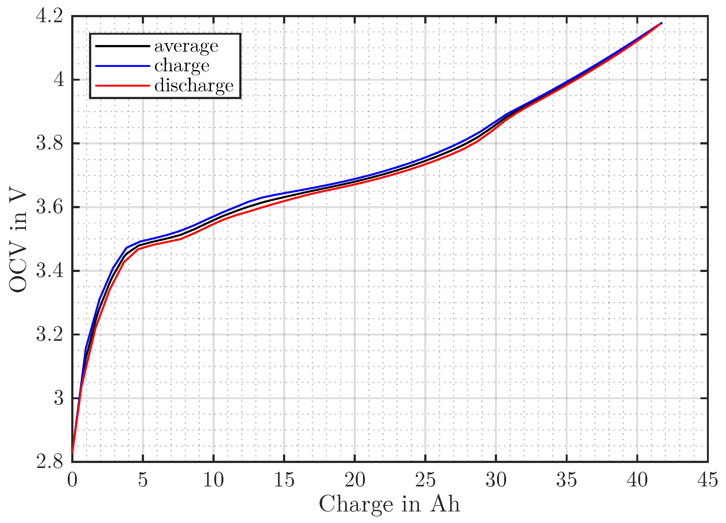
Figure 3 shows the results of an exemplary OCV measurement. In each step, a charge of 1 Ah is charged or discharged. The resting time after each pulse is 1 h.
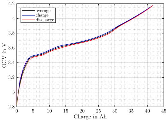
Figure 3.
Exemplary measurement results for the OCV curve of NMC pouch cells recorded at a cell temperature of 22 .
The maximum polarization voltage M of the hysteresis element is defined as half the difference of charge and discharge OCV curves and can be extracted directly from the OCV measurement. It can then be implemented as LUT .
4.2. Model Parameter Identification
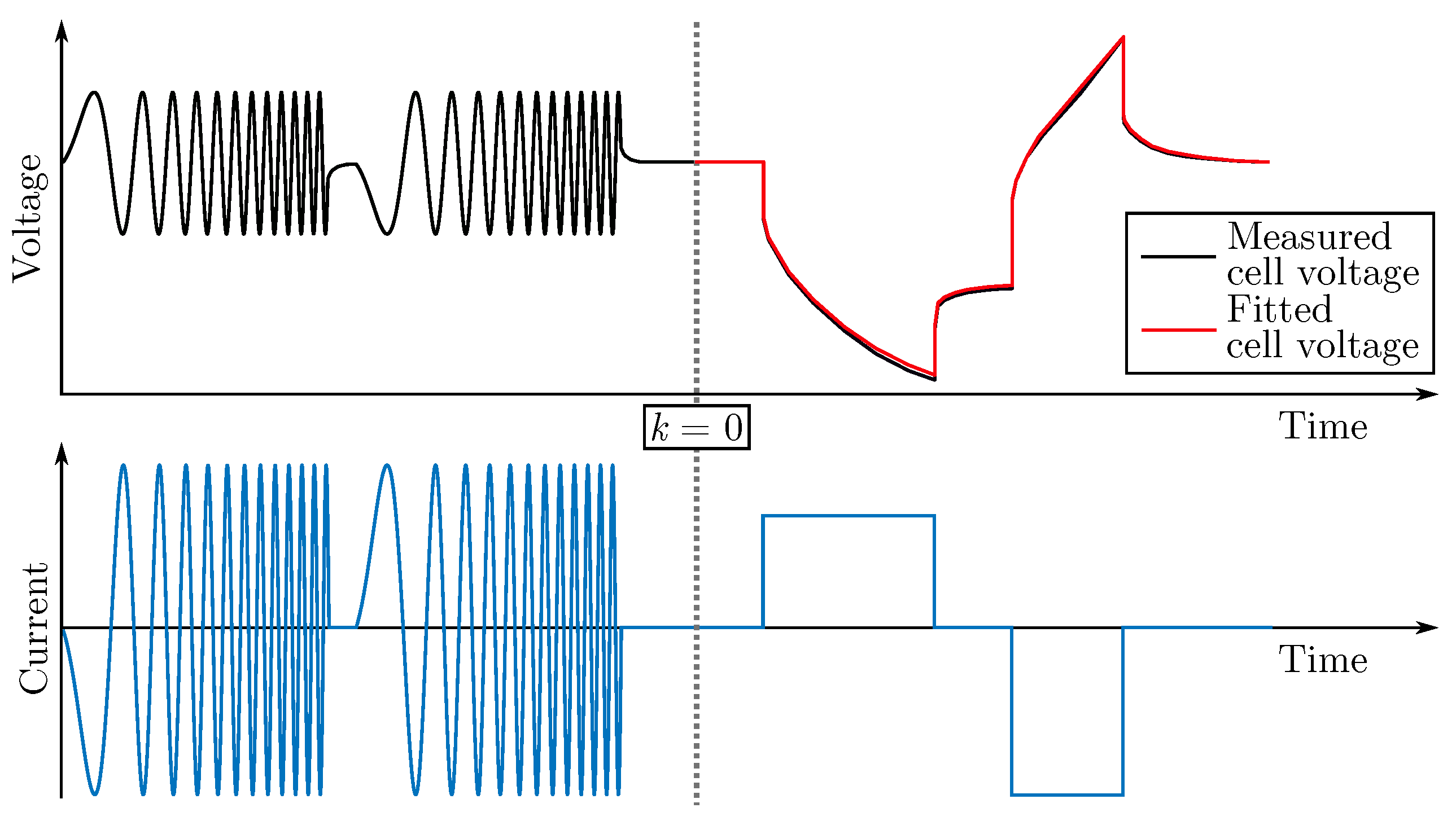
The second necessary characterization step is the estimation of the parameter values. For this purpose, measurement data of the cell need to be collected. Figure 4 shows a possible experiment.

Figure 4.
Schematic view of a model parameterization experiment.
The experiment consists of two phases. First, one or multiple chirp signals bring the battery to a defined state [1]. The effect of these frequency sweeps is that the RC voltages and the hysteresis voltage are almost 0. Then, the measured voltage is approximately equal to the open-circuit voltage , and can be determined.
In the second phase, a rectangular current profile is run. Then the model is fit to the measured voltage. This is done by minimizing the residual sum of squares (RSS) between the predicted cell voltage (according to the model Equation (6)) and the measured voltage v:
For the minimization, common direct search methods may be used. A popular option is the Nelder–Mead algorithm. MATLABs fminsearch is a standard implementation [27].
Since the parameters may vary with SoC, temperature or aging the parametrization experiment should be repeated under different conditions and with multiple cells. The parameters may then be implemented as LUTs. The precision of the parameters is obtained as the standard deviation of the parameter values of identical cells at equal conditions. When the parameters are not implemented as LUTs, the standard deviation calculations should consider the system’s complete operating range.
5. Step-by-Step Guide to Implementation
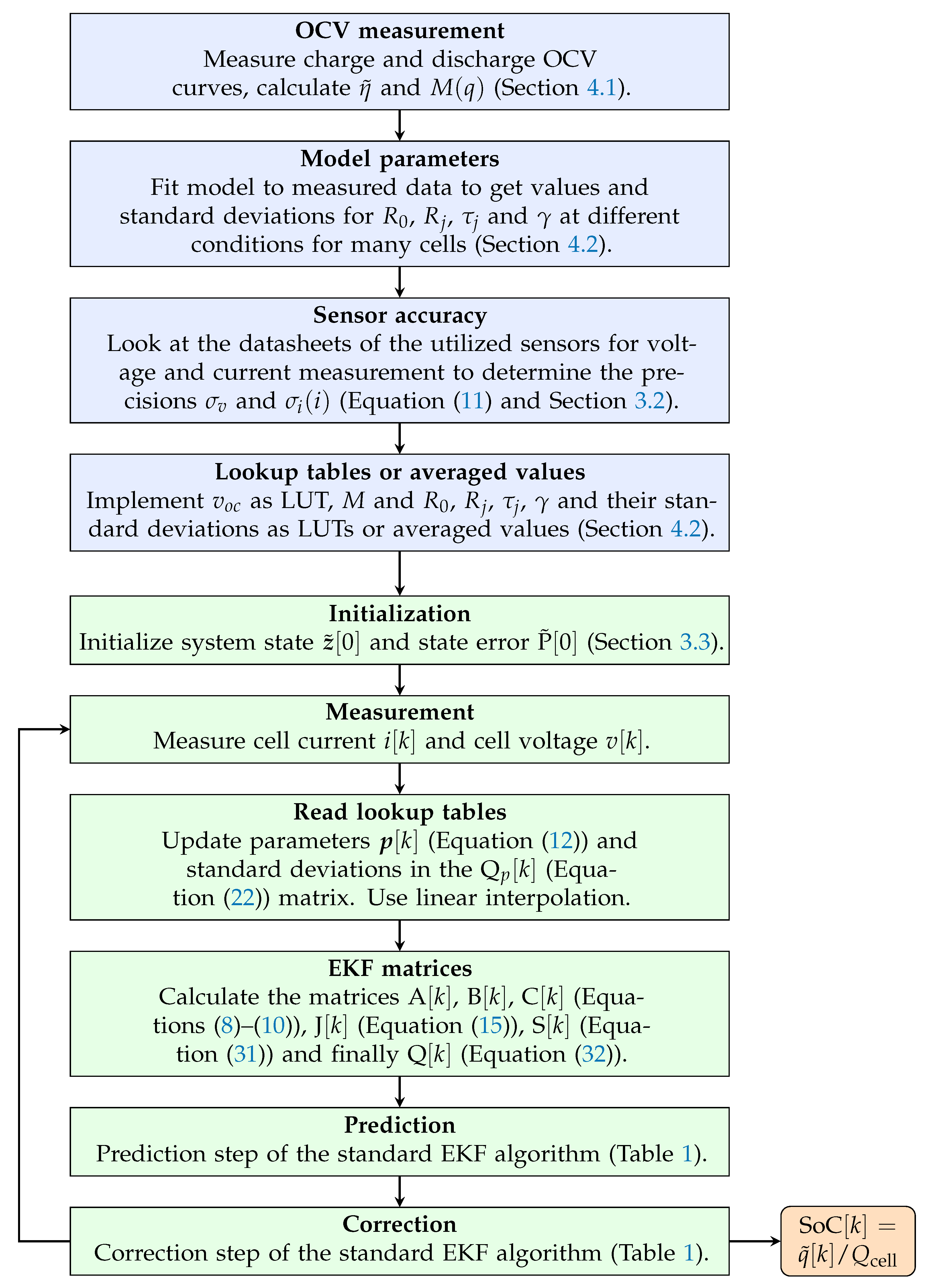
This chapter gives an overview of the necessary steps to get a working EKF implementation for SoC estimation. It summarizes the tasks that have to be performed before and during operation of the battery system. Figure 5 shows this as a step-by-step guide.
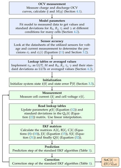
Figure 5.
Steps before (blue) and during operation (green) of the proposed EKF for SoC estimation of a lithium-ion battery cell.
6. Experimental Validation
6.1. Experimental Setup
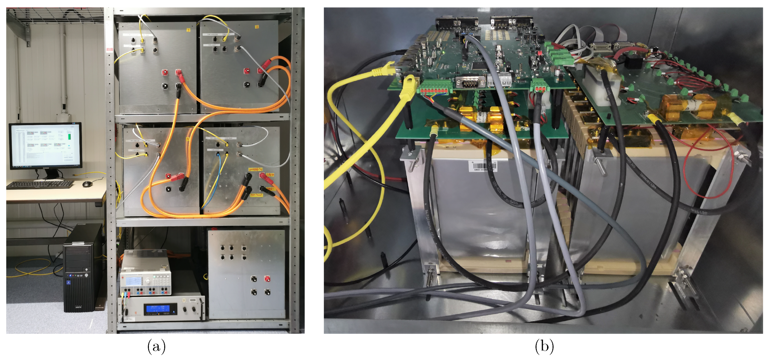
The battery cell which will be evaluated as an example in the following is part of a battery system. The system consists of 96 cells that are connected in series and partitioned into four modules. These modules are organized in a master–slave principle. Each module contains an Infineon AURIX Tricore microcontroller that executes the battery management system (BMS) software, including the proposed EKF algorithm. To connect the battery to the grid, a Delta Elektronika SM 500-CP-90 inverter is used. The setup is shown in Figure 6.

Figure 6.
Experimental setup. (a) Battery system consisting of four battery modules, the SM 500-CP-90 inverter and LabVIEW program for data extraction. (b) Inside view of a battery module.
The BMS measures the cell voltage by an LTC6811 battery monitoring chip that provides a precision of . It measures the cell current by a VAC T60404 fluxgate current sensor with a precision of . The offset of the current sensor is compensated roughly at startup.
6.2. Evaluated Cell
The cell under test is a NMC pouch cell. Its OCV curve is presented in Figure 3. The following cell parameters and standard deviations have been experimentally determined during the preparation of the EKF (see Figure 5):
In the tested version, and M are implemented as LUTs. The standard deviation of M is set to . Due to their comparatively small variation in the examined operating range, the remaining parameters are implemented as constant values with constant standard deviations.
With the safety limits and the , the usable capacity is found from the OCV curve as
6.3. Experiment Procedure
The procedure of the experiment is shown in Figure 7. It mainly consists of a rectangular charge and discharge current profile. After every four repetitions of this profile, the battery is discharged for a longer period and then held in rest for the same time. As a result, the voltage captured at the end of the resting phase can be assumed to be discharged OCV, which yields a reference point for the SoC.
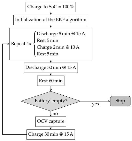
Figure 7.
Procedure of the experiment.
6.4. Comparative Analysis
The results of the proposed EKF SoC estimator (E1) will be compared to three other estimators:
- (E2)
- an EKF with a roughly tuned process noise matrix
- (E3)
- a Coulomb counter with the internal current sensor and the assumed capacity of .
- (E4)
- a Coulomb counter with the precise current sensor of the inverter and cell capacity correction.
E4 is assumed to be the best estimation, and therefore works as the reference SoC. The capacity correction is performed after the experiment based on the measured data. Note that E4 is therefore not applicable for real-time estimation. In contrast, the other three estimators are run in real-time.
For E2, the following matrix is used:
Note that in our implementation, q is in , whereas the voltages are in , which leads to a comparatively large value in the first entry. The order of magnitude for this entry is adapted from [10,12], which proposes a value of 0.01 that is a squared SoC value (variance of the state). This means 10% standard deviation in SoC. However, the Ref. [7] chooses a SoC standard deviation of 0.32%. For comparison, an averaged value of 2 Ah (% SoC) is selected and squared to get as the first entry in . The magnitudes of the voltages strongly depend on the cell-specific resistances, and therefore cannot be adapted from the literature directly. They are roughly estimated from the resistance values and an average current (). The hysteresis voltage is not mentioned in any of the referenced papers, but it is in the order of 10 mV. The estimation of is quite exact, so the corresponding entry in is calculated from the inaccuracy of the current sensor ().
6.5. Results
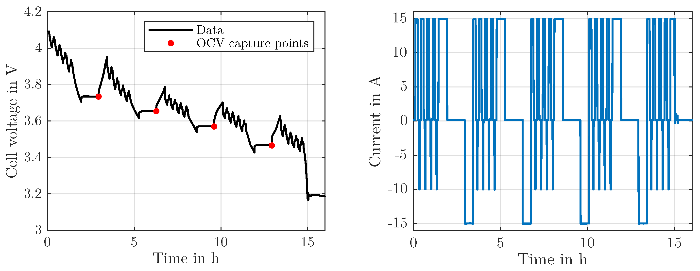
The cell voltage and current measured by the BMS are shown in Figure 8. At , one of the cells in the battery system is fully discharged. Therefore, the tested cell cannot be discharged lower than V. Furthermore, the last 15 A discharge interval (according to Figure 7) cannot be fully executed. Therefore, only four OCV capture points are recorded.

Figure 8.
Measured cell voltage and current during the experiment. In the voltage diagram, the OCV capture points are marked. The current is the signal as measured by the imprecise internal current sensor, which is the same signal used in the EKF algorithm.
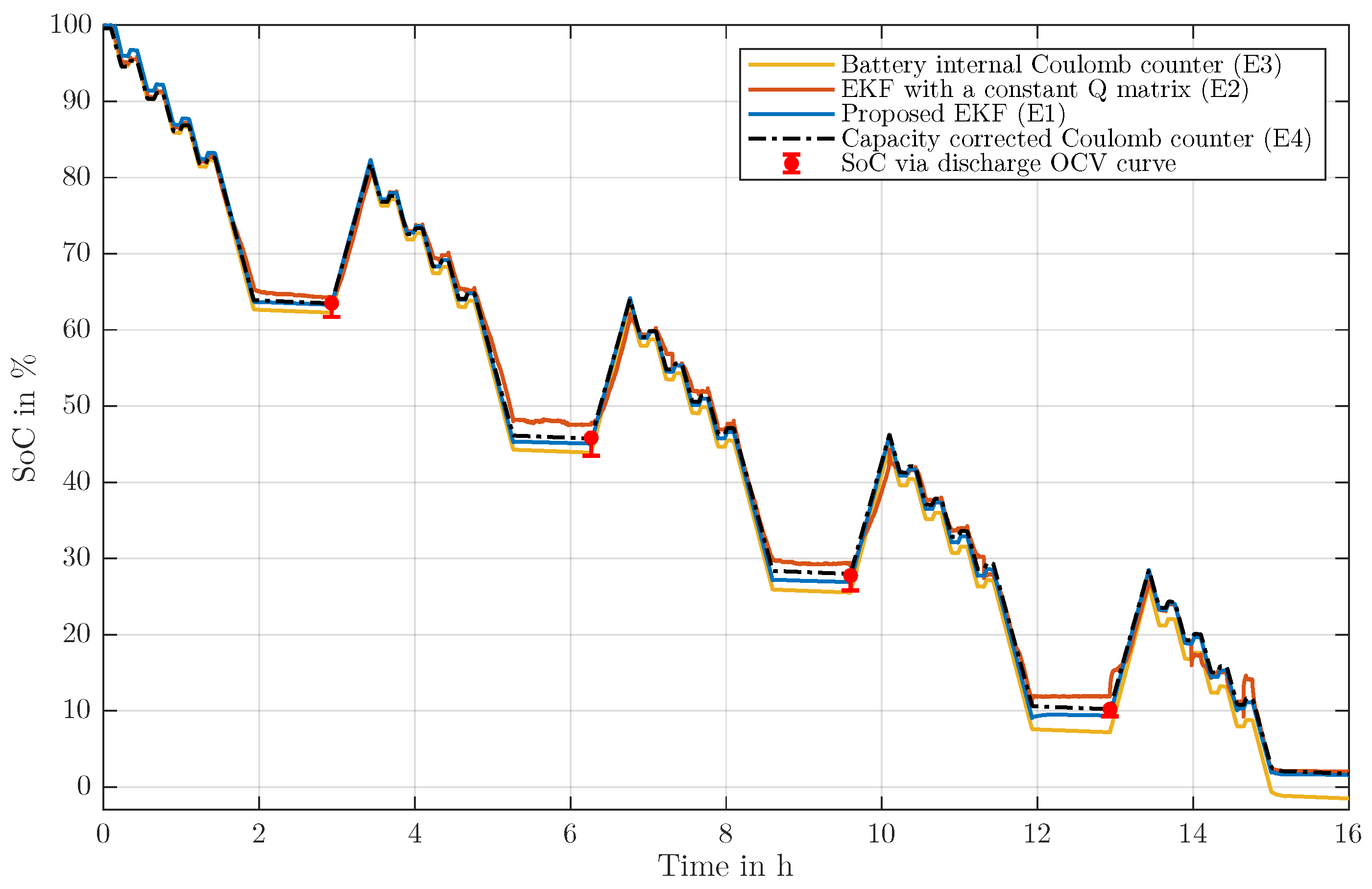
Figure 9 presents the SoCs estimated by the above-mentioned estimators, E1–E4. Additionally, it shows the SoCs calculated via the OCV discharge curve (see Figure 3) evaluated at the OCV capture points. The error bars result from the possibility that the hysteresis element is not fully polarized after a 30 min discharge. The points show the case of full polarization.
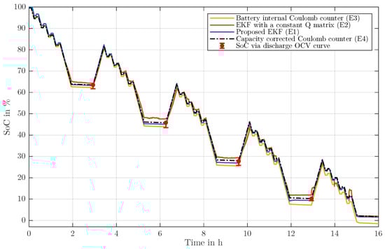
Figure 9.
Estimated SoC for the proposed algorithm (E1) compared to the Coulomb counter based on the internal current sensor (E3), the empirically tuned EKF (E2) and the capacity corrected Coulomb counter based on a more precise current sensor (E4).
The high-accuracy current sensor measured a charge difference of Ah between and the fourth OCV capture point at . The charge difference between these two points in the OCV curve (Figure 3) is only Ah. Therefore, for the gauging of the reference E4, we assume a cell capacity of Ah instead of Ah, as used by E1 to E3.
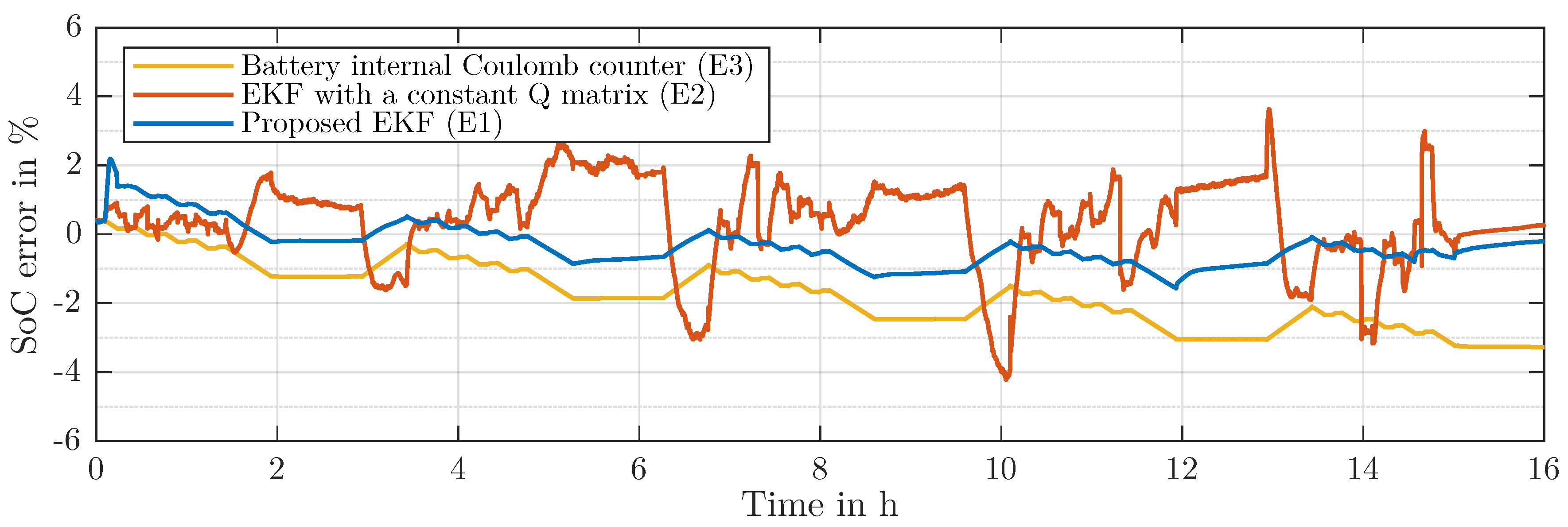
For better visibility of the results, the errors of E1–E3 compared to the reference E4 are depicted in Figure 10.
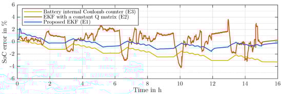
Figure 10.
SoC estimation errors for the estimators E1, E2 and E3 referring to the SoC estimation of E4. The values are plotted in % and due to the unit of the SoC, they are not relative errors.
6.6. Discussion
6.6.1. Validity of the Reference
In the literature, the reference, often called true SoC or real SoC, is gained by Coulomb-counting [10,11,13,21]. This may work for a high-precision current sensor and a perfectly known cell capacity. Capacity and SoC estimation experiments have to be conducted under equal conditions. This is done by monitoring the cell in a controlled temperature chamber (in [21]). In the present system, the cell is in a different condition during the experiment than during the recording of the OCV-SoC dependency described in Section 4.1.
The correction is performed with the fourth OCV point that is captured during the experiment. The fourth OCV point has a small error bar due to the steep region in the OCV curve. Therefore, the reference has a small uncertainty. E4 also hits the three other OCV capture points, which confirms the gauging. The capacity difference of nearly 2 Ah can be explained by the higher temperature in the cell compared to the OCV measurement, which is 29 during the experiment. A possible error of the current sensor also accumulates into the corrected cell capacity.
6.6.2. SoC Estimation Algorithms
Figure 9 shows that the proposed algorithm E1 has the highest accuracy. It only diverges a little from the reference, and hits all OCV capture points at least within each error range. Besides this, Figure 10 confirms the quality of this estimator. The error of the proposed EKF is roughly in a range of ±1% and clearly outperforms the two compared estimators, E2 and E3.
E2 shows an acceptable performance, with an error of a range of ±4%. However, significant fluctuations occur, especially after the resting phases. The performance of E2 might be improved, when the constant matrix is determined more elaborately, such as by trial and error.
The estimation of the Coulomb counter with the internal current sensor (E3) shows the lowest error in the beginning. However, the error grows until the end of the experiment. This is the expected behaviour of a Coulomb-counting estimator. The errors have two origins: the accumulated error in the current measurement and the error of the assumed cell capacity.
7. Conclusions
This work shows the implementation process of a state of charge (SoC) estimator for lithium-ion batteries based on an extended Kalman filter (EKF) using an equivalent circuit model (ECM). The used model includes a hysteresis element to represent the difference between charge and discharge behavior.
For the adjustment of the EKF, methodic approaches are presented. The EKF tuning can be directly derived from sensor and model accuracy. This accelerates development by omitting effortful empirical determination of the process noise matrix . All required steps are presented in a step-by-step guide.
The proposed EKF is experimentally compared to a roughly tuned EKF. It achieves a maximum error of % and good stability. It outperforms the roughly tuned EKF, which shows a maximum error of % and significant fluctuations. The difference in the performance demonstrates how sensitive the EKF reacts to the process noise matrix. Therefore, careful EKF tuning is vital.
8. Outlook
The presented method has been designed to be applicable to other cell chemistries, ECMs, and sensors. This should be experimentally validated in a wide range of operational conditions. This could include increased currents, a wide temperature range, and extended runtimes to facilitate aging processes. We expect that the accuracy of the SoC estimator could be further increased by implementing LUTs for more model parameters instead of using averaged values.
Author Contributions
Conceptualization, B.R., S.B. and T.B.; methodology, B.R.; software, B.R.; validation, B.R. and S.B.; resources, T.B.; data curation, B.R. and S.B.; writing—original draft preparation, B.R. and S.B.; writing—review and editing, B.R., S.B. and T.B.; supervision, T.B.; funding acquisition, T.B. All authors have read and agreed to the published version of the manuscript.
Funding
This research received no external funding.
Conflicts of Interest
The authors declare no conflict of interest.
Abbreviations
The following abbreviations are used in this manuscript:
| BMS | Battery mangement system | ||
| EKF | Extended Kalman filter | ||
| LIB | Lithium ion battery | ||
| LUT | Lookup table | ||
| NMC | Nickel manganese cobalt | ||
| OCV | Open-circuit voltage | ||
| RC | resistor-capacitor | ||
| SoC | State of charge | ||
| Notation | |||
| sampling time | system state | ||
| k | timestep number: | input variable | |
| i | cell current ( for discharge) | measurement variable | |
| v | cell voltage | process noise | |
| coulombic efficiency | measurement noise | ||
| internal resistance | model parameters | ||
| resistance of the j-th RC element | input noise | ||
| capacitance of the j-th RC element | system state error | ||
| time constant of the j-th RC element | Kalman gain | ||
| M | max. hysteresis polarization voltage | linearization state/state | |
| hysteresis rate (unitless) | linearization state/input | ||
| cell capacity | linearization measurement/state | ||
| q | charge in the cell | measurement noise covariance | |
| z | state of charge (SoC): | process noise covariance | |
| open-circuit voltage (OCV) | parameter covariance | ||
| voltage at internal resistance | linearization state/parameters | ||
| voltage at the j-th RC element | input noise covariance | ||
| hysteresis voltage | standard deviation of x | ||
| x is a predicted value | |||
| x is a corrected value | |||
| resting time before initialization |
References
- Plett, G.L. Battery Management Systems, Volume I: Battery Modeling; Artech House: Norwood, MA, USA, 2015. [Google Scholar]
- Meng, J.; Luo, G.; Ricco, M.; Swierczynski, M.; Stroe, D.I.; Teodorescu, R. Overview of Lithium-Ion Battery Modeling Methods for State-of-Charge Estimation in Electrical Vehicles. Appl. Sci. 2018, 8, 659. [Google Scholar] [CrossRef] [Green Version]
- Shrivastava, P.; Soon, T.K.; Idris, M.Y.I.B.; Mekhilef, S. Overview of model-based online state-of-charge estimation using Kalman filter family for lithium-ion batteries. Renew. Sustain. Energy Rev. 2019, 113, 109233. [Google Scholar] [CrossRef]
- Ahmed, R.; Gazzarri, J.; Onori, S.; Habibi, S.; Jackey, R.; Rzemien, K.; Tjong, J.; LeSage, J. Model-based parameter identification of healthy and aged li-ion batteries for electric vehicle applications. SAE Int. J. Altern. Powertrains 2015, 4, 233–247. [Google Scholar] [CrossRef] [Green Version]
- Xing, Y.; He, W.; Pecht, M.; Tsui, K.L. State of charge estimation of lithium-ion batteries using the open-circuit voltage at various ambient temperatures. Appl. Energy 2014, 113, 106–115. [Google Scholar] [CrossRef]
- Hu, C.; Youn, B.D.; Chung, J. A multiscale framework with extended Kalman filter for lithium-ion battery SOC and capacity estimation. Appl. Energy 2012, 92, 694–704. [Google Scholar] [CrossRef]
- Ciortea, F.; Rusu, C.; Nemes, M.; Gatea, C. Extended kalman filter for state-of-charge estimation in electric vehicles battery packs. In Proceedings of the 2017 International Conference on Optimization of Electrical and Electronic Equipment (OPTIM) & 2017 Intl Aegean Conference on Electrical Machines and Power Electronics (ACEMP), Brasov, Romania, 25–27 May 2017; pp. 611–616. [Google Scholar]
- Wang, L.; Wang, L.; Liao, C. Research on improved EKF algorithm applied on estimate EV battery SOC. In Proceedings of the 2010 Asia-Pacific Power and Energy Engineering Conference, Chengdu, China, 28–31 March 2010; pp. 1–4. [Google Scholar]
- Hannan, M.A.; Lipu, M.H.; Hussain, A.; Mohamed, A. A review of lithium-ion battery state of charge estimation and management system in electric vehicle applications: Challenges and recommendations. Renew. Sustain. Energy Rev. 2017, 78, 834–854. [Google Scholar] [CrossRef]
- Chen, Z.; Fu, Y.; Mi, C.C. State of charge estimation of lithium-ion batteries in electric drive vehicles using extended Kalman filtering. IEEE Trans. Veh. Technol. 2012, 62, 1020–1030. [Google Scholar] [CrossRef]
- Zhang, F.; Liu, G.; Fang, L. A battery State of Charge estimation method with extended Kalman filter. In Proceedings of the 2008 IEEE/ASME International Conference on Advanced Intelligent Mechatronics, Xi’an, China, 2–5 July 2008; pp. 1008–1013. [Google Scholar]
- Jokić, I.; Zečević, Ž.; Krstajić, B. State-of-charge estimation of lithium-ion batteries using extended Kalman filter and unscented Kalman filter. In Proceedings of the 2018 23rd International Scientific-Professional Conference on Information Technology (IT), Zabljak, Montenegro, 19–24 February 2018; pp. 1–4. [Google Scholar]
- Lee, J.; Nam, O.; Cho, B. Li-ion battery SOC estimation method based on the reduced order extended Kalman filtering. J. Power Sources 2007, 174, 9–15. [Google Scholar] [CrossRef]
- He, H.; Xiong, R.; Zhang, X.; Sun, F.; Fan, J. State-of-charge estimation of the lithium-ion battery using an adaptive extended Kalman filter based on an improved Thevenin model. IEEE Trans. Veh. Technol. 2011, 60, 1461–1469. [Google Scholar]
- Sepasi, S.; Ghorbani, R.; Liaw, B.Y. Improved extended Kalman filter for state of charge estimation of battery pack. J. Power Sources 2014, 255, 368–376. [Google Scholar] [CrossRef]
- Hariharan, K.S.; Tagade, P.; Ramachandran, S. Mathematical Modeling of Lithium Batteries: From Electrochemical Models to State Estimator Algorithms; Springer International Publishing: Cham, Switzerland, 2017. [Google Scholar]
- Wei, Z.; He, H.; Pou, J.; Tsui, K.L.; Quan, Z.; Li, Y. Signal-Disturbance Interfacing Elimination for Unbiased Model Parameter Identification of Lithium-Ion Battery. IEEE Trans. Ind. Inform. 2020, 1. [Google Scholar] [CrossRef]
- Hu, J.; He, H.; Wei, Z.; Li, Y. Disturbance-Immune and Aging-Robust Internal Short Circuit Diagnostic for Lithium-Ion Battery. IEEE Trans. Ind. Electron. 2021, 1. [Google Scholar] [CrossRef]
- Zhou, D.; Yin, H.; Xie, W.; Fu, P.; Lu, W. Research on online capacity estimation of power battery based on ekf-gpr model. J. Chem. 2019, 2019, 5327319. [Google Scholar] [CrossRef] [Green Version]
- Diab, Y.; Auger, F.; Schaeffer, E.; Wahbeh, M. Estimating lithium-ion battery state of charge and parameters using a continuous-discrete extended kalman filter. Energies 2017, 10, 1075. [Google Scholar] [CrossRef] [Green Version]
- Bian, X.; Wei, Z.; He, J.; Yan, F.; Liu, L. A two-step parameter optimization method for low-order model-based state of charge estimation. IEEE Trans. Transp. Electrif. 2020, 7, 399–409. [Google Scholar] [CrossRef]
- Plett, G.L. Battery Management Systems, Volume II: Equivalent-Circuit Methods; Artech House: Norwood, MA, USA, 2015. [Google Scholar]
- Kalman, R.E. A New Approach to Linear Filtering and Prediction Problems. Trans. ASME J. Basic Eng. 1960, 82, 35–45. [Google Scholar] [CrossRef] [Green Version]
- Schneider, R.; Georgakis, C. How to not make the extended Kalman filter fail. Ind. Eng. Chem. Res. 2013, 52, 3354–3362. [Google Scholar] [CrossRef]
- Ma, W.; Qiu, J.; Liang, J.; Chen, B. Linear kalman filtering algorithm with noisy control input variable. IEEE Trans. Circuits Syst. II Express Briefs 2018, 66, 1282–1286. [Google Scholar] [CrossRef]
- Soto, A.; Berrueta, A.; Sanchis, P.; Ursúa, A. Analysis of the main battery characterization techniques and experimental comparison of commercial 18650 Li-ion cells. In Proceedings of the 2019 IEEE International Conference on Environment and Electrical Engineering and 2019 IEEE Industrial and Commercial Power Systems Europe (EEEIC/I&CPS Europe), Genova, Italy, 11–14 June 2019; pp. 1–6. [Google Scholar]
- Optimizing Nonlinear Functions. Available online: https://de.mathworks.com/help/matlab/math/optimizing-nonlinear-functions.html (accessed on 2 May 2021).


Publisher’s Note: MDPI stays neutral with regard to jurisdictional claims in published maps and institutional affiliations. |
© 2021 by the authors. Licensee MDPI, Basel, Switzerland. This article is an open access article distributed under the terms and conditions of the Creative Commons Attribution (CC BY) license (https://creativecommons.org/licenses/by/4.0/).