A Study on the Effect of Ignition Timing on Residual Gas, Effective Release Energy, and Engine Emissions of a V-Twin Engine

Abstract

The ignition timing of an SI engine is a critical parameter. The influence on residual gas, effective release energy, and emissions characteristics of ignition timing for the V-twin engine is investigated in this research. For this purpose, an experiment system was built with a dynamometer, and a model of the simulation was created. In this research, the ignition timing was varied from 10 to 45 degrees BTDC under full load operating conditions, with engine speeds ranging from 3000 to 10,000 rpm. Based on the output data, ignition timing has a major impact on the proportion of residual gas, efficient release energy, performance of the engine, and the emission characteristics. The smallest proportion of residual gas was 0.07% at 8000 rpm and ignition timing of 10 °CA. At 15 °CA of ignition timing, the highest efficient release energy was 0.817 kJ at 4000 rpm, while at 8000 rpm and 25 °CA of ignition timing, it was 0.8305 kJ. At 6000 rpm, the greatest braking torque of the engine was 21.57 Nm, while the minimal BSFC was 343.821 g/kWh. The nitrogen oxide emission and HC emission increase with the advanced ignition timing, but CO emission decreases.

1. Introduction

Global population growth and technological advancements have resulted in a significant increase in the number and use of road vehicles that are powered by fossil fuels. Problems associated with the depletion of fossil fuels and increasing environmental pollution are on the rise due to this rapid development [1]. Due to these issues, better thermal efficiency and lower emissions from engines are increasingly mandated [2]. Many factors influence the emission characteristics and performance of SI engines [3,4]; ignition timing is among the most important [5]. Ignition timing is strongly influenced by flame speed, which has a significant impact on the SI engine performance [6].

The thermodynamics of an engine with high ignition retardation was studied by Chan and Zhu, who focused on the impact of a retarded spark on pressure distribution in the engine cylinder. Temperature of the gas inside the cylinder and trapped mass were also calculated under different spark timing conditions [7]. To analyze the effect on the burning rate and pressure of the gas in the cylinder of the spark timing and the composition of the fuel and equivalence ratio for a natural gas engine, a model for Zero-D two zone thermodynamics was built by Soylu and Van Gerpen [8]. Under a variety of operating conditions, characteristics of burning rates are analyzed to clarify the initiation, propagation, and termination of the flame. Hedfi et al. studied bioethanol combustion and discovered that retarded spark timing leads to higher temperature and pressure of the gas mixture in the cylinder [9]. The optimal injection and ignition timing for a methanol engine was investigated by Li et al. They discovered that these timings had a major impact on methanol engine combustion and exhaust emissions [10]. A fuel injection system with a high-pressure injector and with a hollow cone spray was studied by Beatrice et al. [11,12]. They report that high injector pressure reduces peak firing pressure, increasing fuel efficiency.

In past years, the battery ignition manifold’s centrifugal and vacuum regulators were used to control ignition timing. Manufacturers are being forced to produce increasingly complicated engines, and their parts as emissions regulations tighten. There are a number of options for meeting the emission standards. One method involves incorporating contemporary structural components: injection systems with high pressure, all electronically controlled ignition systems, etc. [13]. To better satisfy user requirements and operating conditions, electronic controls are increasingly replacing mechanical controls. Factors such as speed, load, temperature, and change of fuel type in an engine are the operational conditions, particularly given the penchant for biomass fuels or biofuels in recent years. Alcohol-based biofuels (for SI engines) have a higher octane rating compared with gasoline because they contain oxygen [14]. The higher octane number of the fuel, in addition to its improved anti-knocking properties, can change the timing of ignition required to reach decreased emissions. At high loads, an earlier ignition timing helps to decrease the temperature of exhaust gas [15,16]. As a result, adding fuel to the mixture in order to prevent engine parts from rising in temperature is unnecessary. The engine would run more efficiently if the dose injected were reduced [17]. Lower fuel consumption is expressed in quality of ignition control based on conditions of operation and impacts overall efficiency, leading to increased engine power [18]. The quality of the combustion is a reflection of the engine’s efficiency. In addition, the change in concentration of exhaust gases such as NOx, CO, and unburned HC is due to the impact of changing ignition timing [19].

In spark ignition engines, the formation of flame, premature burning, and behaviors of emissions are all influenced by ignition timing [20]. The impact of timing for spark on the combustion of an engine fueled with hydrogen was studied by Shi et al. [21]. They discovered that with the advanced spark ignition angle, the brake thermal efficiency initially increases followed by a decline. NOX, HC, and CO emissions also decreased with retarded spark timing. NOX emissions increase as the fraction of hydrogen volume increases, whereas HC and carbon monoxide are reduced. The impact of adding a high percentage of hydrogen on the performance of engines fueled by hydrogen–gasoline blends was studied by Elsemary et al. [22]. The finding was that at an ignition timing of 30 °CA BTDC, the consumption of fuel is reduced, and the thermal efficiency improves [23]. Zhang et al. studied the impact of a spark timing hydrogen/methanol engine on combustion and emissions with the coefficient of excess air at 1.20 and discovered that with increased spark advance angles, after the initial increase, the indicated thermal efficiency begins to decline. Along with the more advanced ignition timing, the flame production time lengthens while the flame propagation period shortens. After hydrogen is added, unburned hydrocarbon and carbon monoxide fall [24]. Syed Yousu Fuddin investigated the impact of the spark timing and compression ratio on engine-fueled hydrogen–ethanol. The researchers showed that by increasing the fraction of hydrogen, the thermal efficiency and mean effective pressure improved for a given ignition time.

Ignition timing is a critical operating parameter that affects the performance and emission characteristics of SI engines. However, little work has been reported addressing the impact of ignition timing on the proportion of residual gas and efficient release energy for motorcycles. Thus, it is necessary to study the impact of ignition timings on V-twin engine performance and emissions characteristics, as well as to assess the optimal ignition timing for maximum brake torque and minimum BSFC.

2. Experiment Setup and Material

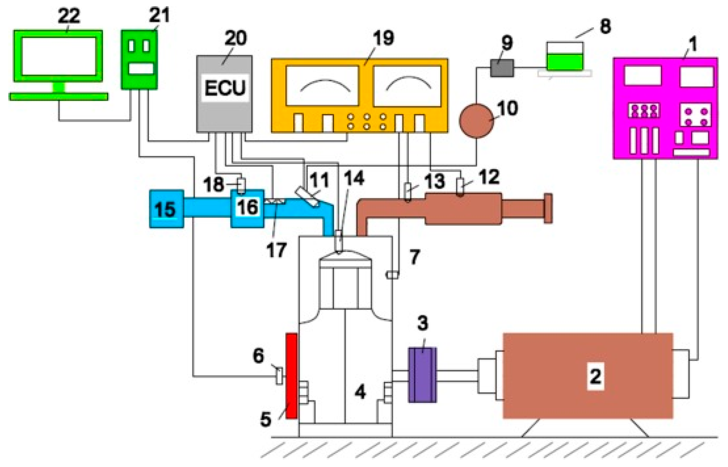
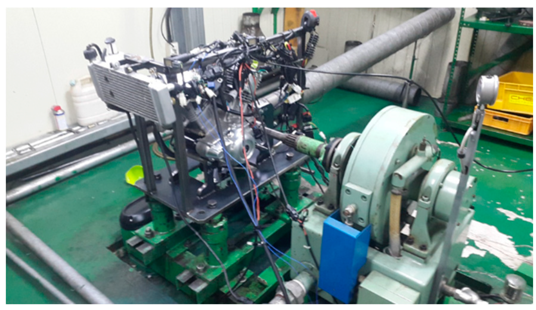
2.1. Experiment Setup

Schematic representation of setup for experiments and the engine testing system are depicted in Figure 1 and Figure 2, respectively. There are 22 components to this experiment system. The torque resistance for the experiment was supplied by a controller for dynamo testing systems (1) and a dynamometer from the AVL company (MCA325MO2) (2). Engine and dynamometer are connected by coupling (3). An encoder autonics (6) and sensor for temperature (7) were mounted on the flywheel (5) and the engine (4), respectively. The fuel travels to the fuel filter (10) from the fuel tank (8) and then to the fuel pump (9), where it is injected into the fuel injectors (11). The box to filter the air (15) and the throttle allow air to enter the intake pipe (16). The air heater regulated the temperature of the intake air (17). The analyzer for exhaust gases and transducer for cylinder pressure (19), ECU (20), data collection (21), and computer (22) receives signals from the sensor that detects oxygen quality (12), sensor for temperature of exhaust gas (13), sensor for cylinder pressure (14), angle of the throttle, and sensor for measuring air mass (18).

The engine used in the experiments is a V-twin engine (4-strokes, four intake valves, and four exhaust valves). The engine is installed for the motorcycle. This engine has a system of injection on the intake manifold and a piston with a flat top. Two camshafts are used in the experimental engine, one for inlet valve control and one for exhaust valve control. The conditions of experiment were defined with a volume fraction of 11.8:1.0, the air-to-fuel coefficient is 13.6, and the temperature of the testing system surroundings should be between 29.5 and 30 degrees. Air is used as a coolant; the lubrication temperature was kept at 80 degrees. The fuel supply system holds the fuel pressure between 333 kPa and 363 kPa. As the engine was running, the throttle opening angle was set to completely open. Under different speeds of the engine, the state of the experiment is steady with constant spark advance. Before the analysis, all of the equipment was calibrated.

The specifications of the engine are provided in

Table 1. The engine specifications.

Parameter	Unit	Value
Engine model	-	Four stroke, Spark ignition
Number of cylinder	-	2(V-Twin)
Compression ratio	-	11.8:1
Bore	mm	57
Stroke	mm	53.8
Connecting rod	mm	107.9
Intake valve	-	2
Exhaust valve	-	2
Cooling system	-	Air cooled

2.2. Simulation Model Setup

It would be very difficult to calculate residual air remaining and the effective release energy in our experiment. Simulation is, for that reason, a very strong and useful technique for addressing this issue. AVL-boost is a simulation program for engine cycles and gas exchange that allows one to create a model of the whole engine by selecting elements from a toolbox and linking them with pipe elements. In the automobile industry, AVL-boost is used to simulate engines accurately. It can model a large variety of types and sizes of engines, such as two-cycle, four-cycle, diesel, and gasoline.

The simulation elements reflect the experimental engine’s components in Figure 3. The simulation elements are employed to investigate the properties of engine components. For the conditions of the experiment, the element E1 represents that the engine has been established in a steady state or in a transient state. Another factor was that the display screen MNT1 is absent in the engine under consideration. Through this monitor feature, investigators can see desired information including torque, ratio of residual gas, peak fire pressure, and effective release energy. The two factors SB1 and SB2 reflect the borders of the inlet and exhaust tubes, respectively. The factor CL1 in the experiment plays a role as a system air filter. The element TH1 was established from the throttle opening angle, which was completely opened during engine operation. The element restrictions R1, R2, and R3 take on reducing the pressure of the air stream through the intake and exhaust manifold (from 1 to 21). The contiguous elements from J1 to J6 take charge of allocating the gathered airflow in the tube. Some of the main indicators of airflow include velocity, temperature, and mass flow rate; they can be measured directly through MP1 and MP2. Fuel from the injectors I1 and I2 supply the cylinders C1 and C2, respectively.

To measure characteristics of heat release, the simulated model of the engine was built using the combustion function by Vibe:

$$\frac{dx}{d\alpha }=\frac{a}{\Delta \alpha }\left(m+1\right)y^m e^{-a.y\left(m+1\right)}$$

(1)

$$dx=\frac{dQ}{Q}; y=\frac{\alpha -{\alpha }_0}{\Delta {\alpha }_c}$$

where:

Q is total fuel heat input (W);

α is the crank angle (deg);

α₀ is the start of combustion (deg);

∆α₀ is combustion duration (deg);

m is shaped parameter (–).

The integral of the Vibe feature provided the mass faction burned χ:

$$x={\displaystyle \int }\frac{dx}{d\alpha }d\alpha =1-e^{-a.y\left(m+1\right)}$$

(2)

Woschni’s model was used to determine how much heat was transferred in the combustion chamber:

$$Q_T=A.q_{coeff} \left(T_c-T_w\right)$$

(3)

where:

Q_T is heat lost to the wall (W/m²);

A is the total surface area of the cylinder head, piston, and cylinder (m²);

q_coeff is heat transfer coefficient (W/m² K);

T_c is combustion gas temperature (K);

T_w is the wall temperature of the cylinder (K).

Engine efficiency is calculated through Equation (4):

$${\eta }_{th}=1-\frac{1}{r^{\gamma -1}}$$

(4)

$$\gamma =\frac{C_p}{C_v}$$

where:

η_th is theoretical engine efficiency;

r is the compression ratio;

γ is the specific heat ratio (depending on monatomic gas or diatomic gas);

C_p is specific heat capacity with constant pressure (J/kg K);

C_v is specific heat capacity with constant volume (J/kg K).

Equation (4) was used to measure the residual gas fraction:

$$x_{SOC}^{cp}=\frac{{{\displaystyle \int }}_{V_c}^V\rho x^{cp} dV}{{{\displaystyle \int }}_{V_c}^V\rho dV}$$

(5)

Equations (6) and (7) are used to determine the concentration of N₂O and the rate of NO production, respectively:

$$C_{\mathrm{N}2\mathrm{O}}={\mathrm{1.1802.10}}^{-6} T^{0.6125} e^{\frac{9471.6}{T}} C_{N_2} \sqrt{P_{O_2}}$$

(6)

$$r_{NO}=2 C_p C_k \left[1-{\lambda }^2\right] \frac{r_1}{1+\lambda R_1} \frac{r_4}{1+R_2}$$

(7)

$$\lambda =\frac{C_{NO,act}}{C_{NO,equ}} \frac{1}{C_p};R_1=\frac{r_1}{r_2+r_3};R_2=\frac{r_4}{r_5+r_6}$$

Equation (8) is used to calculate CO production:

$$r_{CO}=C_{Const} \left(r_1+r_2\right)\left(1-\theta \right)$$

(8)

$$\theta =\frac{C_{NO,act}}{C_{NO,equ}}$$

Equation (9) was used to measure the mass of unburned HC:

$$m_{HC}=\frac{P_c V_{crevice}M}{R T_{piston}}$$

(9)

3. Results and Discussions

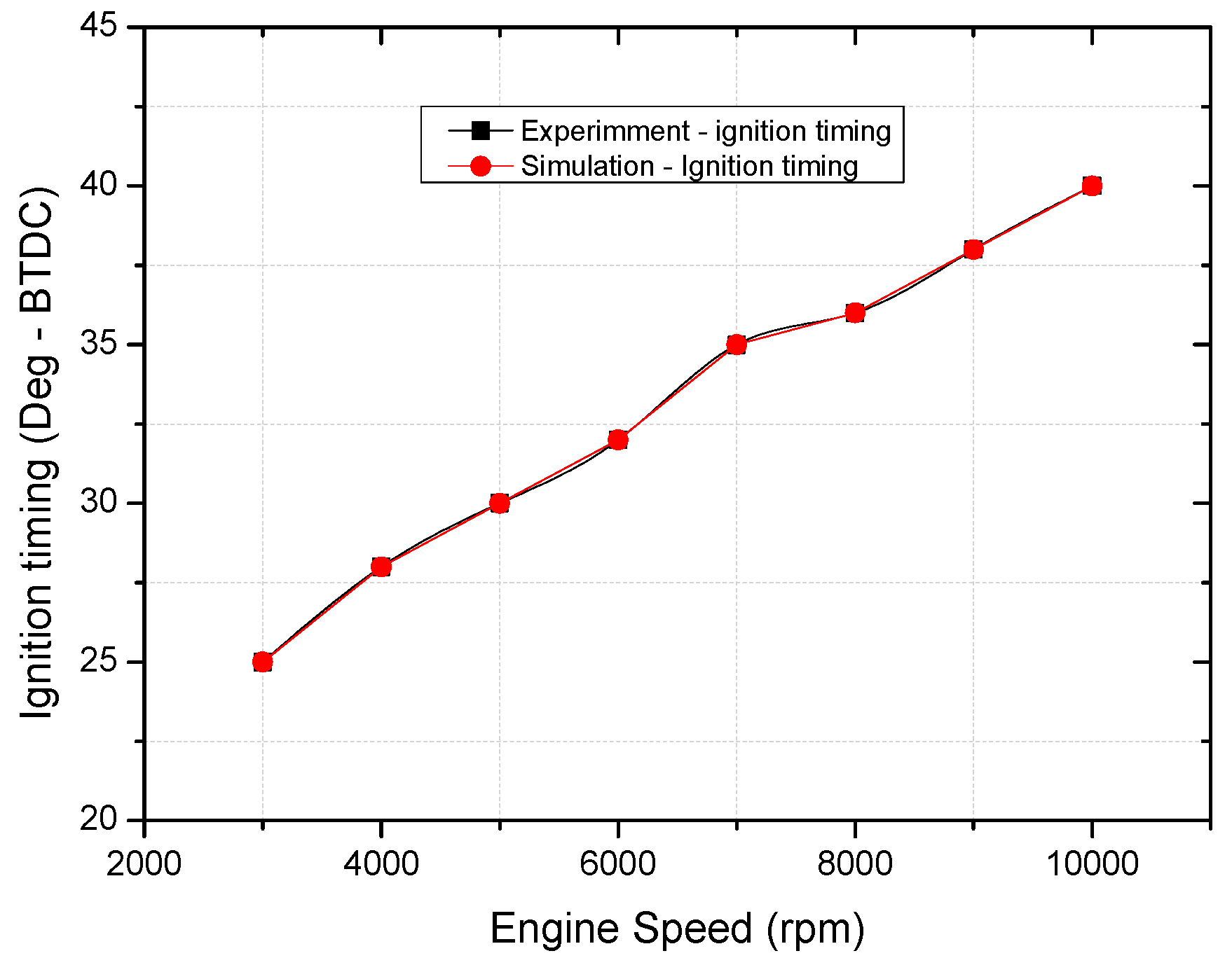
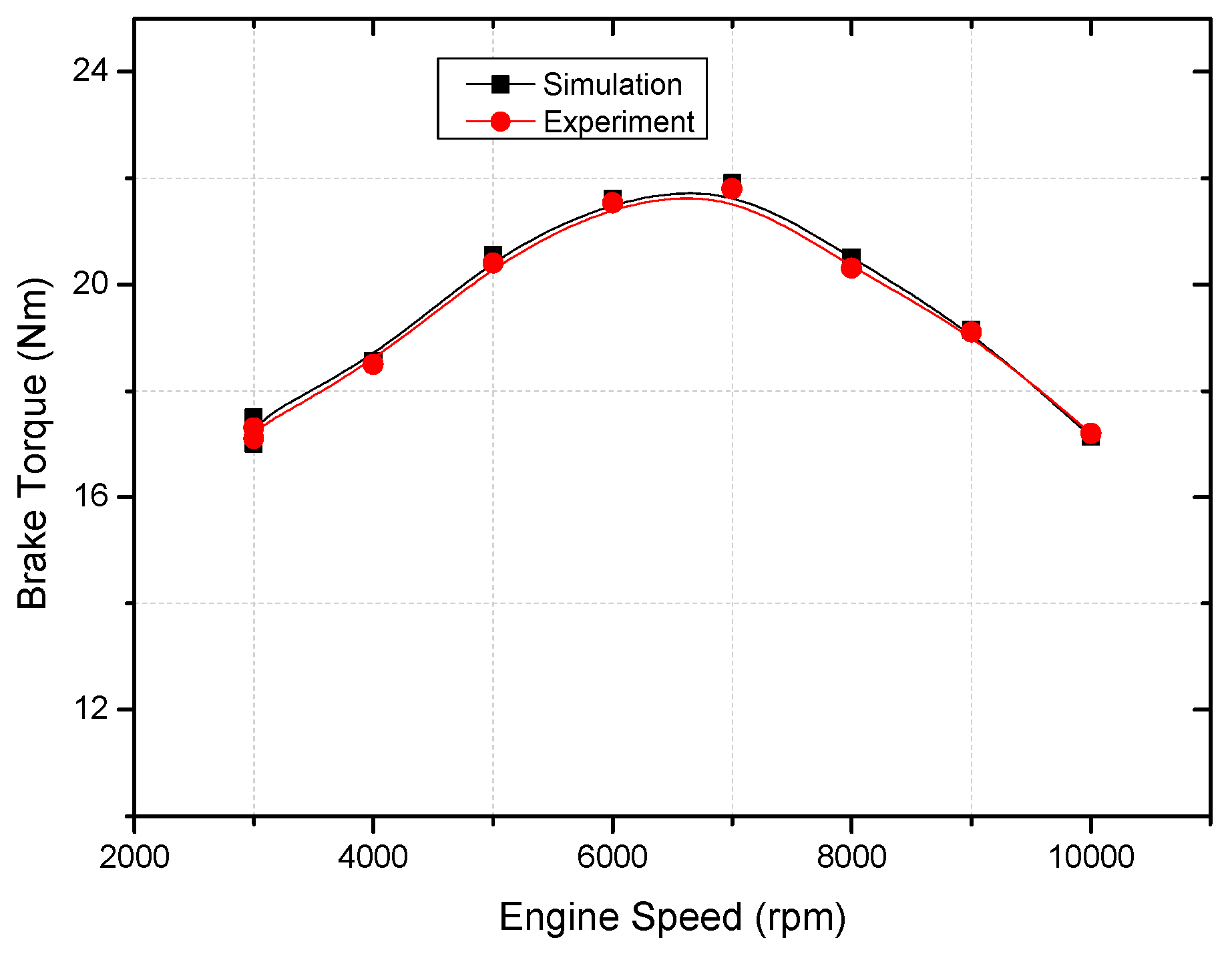
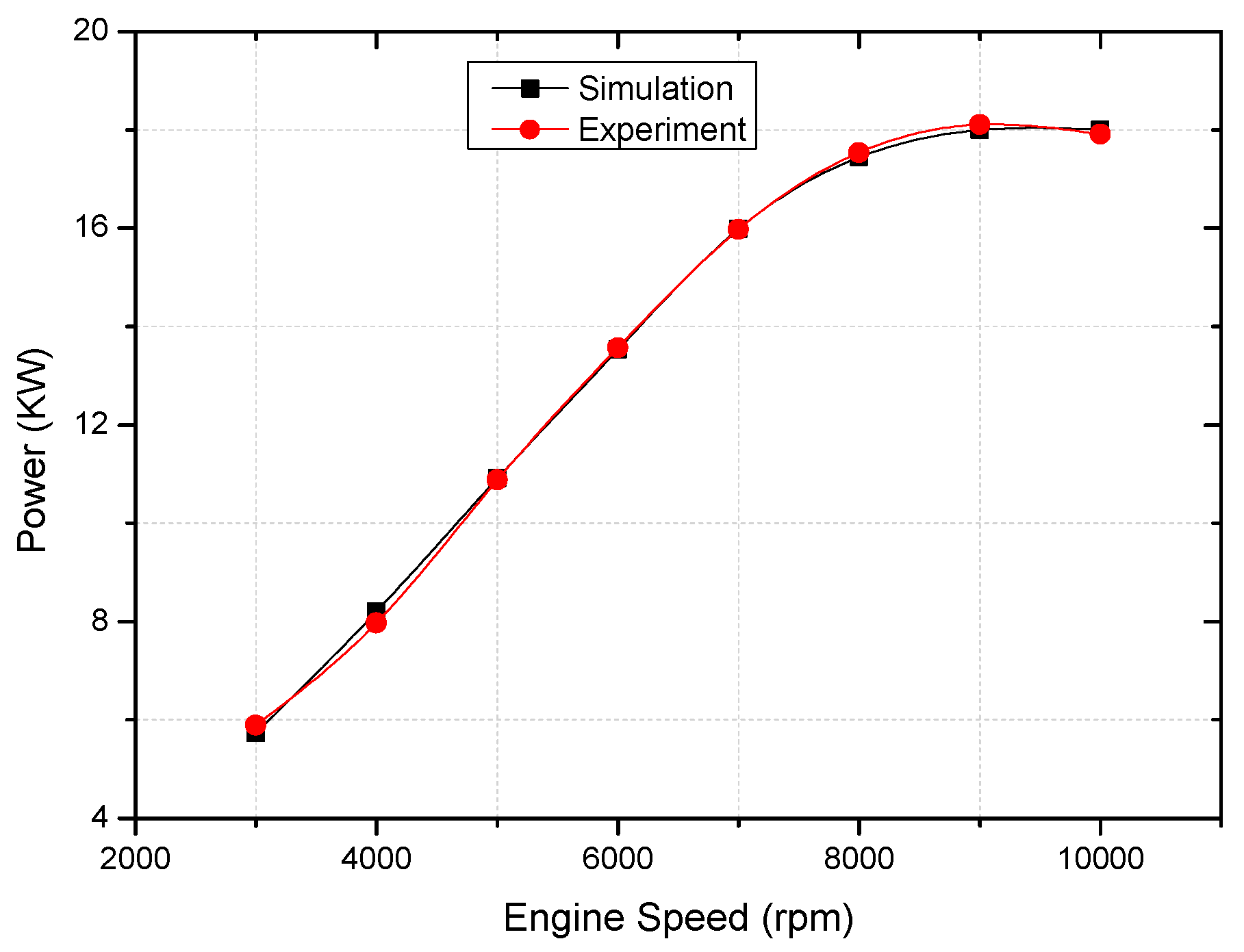
3.1. Model Validation

The aspects and robustness of our research were demonstrated by both theoretical and experimental tests, represented by red and black lines in Figure 4. Calibration and validation equipment (simulated model) help avoid imprecise measurements in estimating ignition time. The factors that are taken into account in the assessment of simulated model include values of engine specification such as bore, stroke, path length, and diameter of intake and exhaust pipe, as well as a list of values in experimental conditions.

Overall, the ignition time values in both investigations (simulation and experiment) are relatively consistent with each other (Figure 4), denoting confidence that the result for the index was verified. The result is, moreover, a good sign for the other indicators that will be implemented in the upcoming figures.

The air mass flow in the simulated model was adjusted by means of changing major coefficients known as intake pipe, throttle, intake ports, and exhaust ports. Results from simulation and experimental tests are presented in Figure 5. their values are compatible with insignificant differences. The highest different value is a very small number (1.42%) at 6000 rpm, which is acceptable when seen as an average value of the air mass flow during the experiment.

Errors in measurement of the engine brake torque and power were restricted by support from the accurate ratio between air-fuel and engine friction. On the other hand, the m parameter in Equation (3) is used as a key in reducing errors. Figure 6 shows the results for brake torque indicator in both cases (simulation and experiment). The numerical simulation values are similar with experimental data at each velocity. Interestingly, at 7000 rpm, the brake torque reached the peak at 21.8 Nm. The difference between theoretical and experimental cases was approximately 0.9%.

Engine power results are demonstrated in Figure 7. The best engine power was 18.11 kW at 9000 rpm. The phenomenon in both cases was not out of our prediction, with the differences being less at each speed of the engine and only a 0.59% difference being reported in the indicator as the highest value difference.

By making good use of the many compatibilities, experimental and simulation results have been meticulously formulated and linked together to establish a stable model, making it a precise method useful to efficiently predict the engine performance. Furthermore, implementing the model makes it possible to learn more about the effect of air residue on the engine performance, as well as on engine emission characteristics.

3.2. Results

The results show the effect of ignition timing on residual gas, effective real energy, and parameters such as BSFC, IMEP, BSFC, peak firing temperature, brake torque, and engine power.

Figure 8 shows the impact of ignition time on the residual air indicator. At an engine speed of 8000 rpm, increasing ignition time (from 10 to 45 degrees) results in the residual air going up from 0.07% to 0.26%. On the other hand, reducing engine speed at 6000 rpm causes the residual air rate to increase by a very small number (about 1–1.05%). However, at a lower engine speed (4000 rpm), this ratio fluctuated slightly. The minimum ratio was 0.54% under the specific ignition time condition (30 °CA). This can be attributed to the average and higher speed of the piston, which leads to a faster and cleaner moving out of the residual air. From the process, we need to consider the upcoming intake stroke, and it predicts a reduction in fresh air flow entering the combustion chamber.

Figure 9 presents the effect of ignition timing on peak firing temperature. As the ignition timing increases, the peak firing temperature increases. It can be explained that when ignition timing is increased, with the lateness of the ignition timing, there will be more time for the mixture to blend better. This leads to the mixture being more evenly mixed, thereby leading to a complete combustion. The maximum peak firing temperature was 2993.26 K at 45 °CA of ignition timing as engine speed was 6000 rpm.

Figure 10 and Figure 11 illustrate the impact of ignition timing on peak firing pressure and peak pressure rise. The peak firing pressure and peak pressure rise show the same trend with the peak firing temperature when increasing the timing of ignition. The peak firing pressure and peak pressure rise reached the maximum when the revolution of the engine was 6000 rpm and the timing of ignition was 45 °CA. The maximum values are 108.36 bar and 9.71 bar/deg, respectively.

The impact of ignition timing on effective release energy is presented in Figure 12. When the engine revolution speed was 6000 rpm and 8000 rpm, the values of effective release energy trend upward. In particular, when the revolution speed was 6000 rpm, the effective release energy increased quickly before reaching its peak. Following that, a decline was found. When the engine speed was 4000 rpm, the effective release energy decreased sharply before steadily increasing. The maximum efficient energy release is an important metric that cannot be ignored in any engineering test. In our study, the coefficients change continuously as the engine speed changes. Two hypotheses are assumed. Firstly, the ignition time occurs late, resulting in too short of a burning time, so the fuel cannot be completely converted into heat. In contrast, if the burning time is long because of the advanced ignition time, energy in the form of heat will be significantly lost. This explains why the efficient release energy is sharply increased at the first stage and is then controlled by ignition time. Secondly, the combustion reacts in a short time since energy occurs simultaneously at TDC. In order to optimize the thermal energy for efficiency, the total heat release must be concluded in a short time. This leads to the increased frequency of the energy release to be close with the Otto cycle. Moreover, the range of engine velocity plays a role in driving the total energy release “heat” [25]. The best effective release energy at 4000 rpm and 15 °CA of ignition timing was 0.81725 kJ. Additionally, the best effective release energy at 6000 rpm and 8000 rpm was 0.83374 kJ and 0.83407 kJ at 45 °CA and 25 °CA of ignition timing, respectively.

The effects of ignition time on BMEP and IMEP are presented in Figure 13 and Figure 14, respectively. The phenomenon can be observed under two stages. In the first stage, BMEP and IMEP rapidly increase to a clear peak value. In the next stage, the trend reverses steadily. At each revolution speed, the optimal values of BMEP and IMEP during the same time the ignition time reached its peak were reported. This can be explained by the phenomenon that the moment of ignition occurs simultaneously with the release of energy. Some noteworthy values are the ignition time benchmark (optimal value) obtained at 9.49 bar on BMEP and 12.09 bar on IMEP at 4000 rpm—20 °CA. Under other conditions (6000 rpm—30 °CA), the optimal value was 9.87 and 12.82 bar on BMEP and IMEP, respectively. Increasing at 8000 rpm and 30 °CA of the ignition time, BMEP and IMEP reached 9.62 and 12.12 bar. This denotes that the ignition time clearly depends on these conditions.

The effect of ignition time on BSFC is shown in Figure 15. The trend is opposite to that of BMEP and IMEP. During the first stage, BSFC went down continuously until it met the minimum value, and then the trend reversed. One interesting phenomenon to note is that the trends of BMEP and BSFC run in opposite directions [26]. At each engine speed, a set of numbers including ignition time and fuel consumption is reported. The minimal value of BSFC was reported with 401.89 g/kWH at 4000 rpm and 20 °CA. At the same speed (6000 rpm) and increasing at 25 °CA of the ignition time, BSFC reached 343.82 g/kWh. If the set of numbers is increased to 8000 rpm and 35 °CA, the BSFC value is 371.69 g/kWh.

Figure 16 and Figure 17 also highlight the relationship of ignition time on power and braking torque, respectively. When the ignition time had an increase on BMEP, the trend of engine brake torque was consistent with the engine power trend. Their trends clearly divide into two stages. In the early stage, they rose steadily until reaching their optimal values. The second stage can be observed with reverse trends that occurred at the same ignition time, while the ignition time continuously went up. Furthermore, at each revolution speed, the specific values of the combustion time and optimal performance are presented. At 4000 rpm and 20 °CA, the maximum engine braking torque was 20.74 Nm, while the maximum power was 8.96 kW. At 6000 rpm, their values were 21.57 Nm and 13.55 kW under 30 °CA ignition time, respectively. At higher speed (8000 rpm) and 35 °CA, 21.01 Nm and 17.6 kW were respectively reported.

Figure 18 presents the impact of ignition timing on nitrogen oxide emission. The nitrogen oxide emission increases with the advanced ignition timing owing to the increased peak firing temperature. The nitrogen oxides are more affected by the peak firing temperature. The retarded ignition timing is said to decline nitrogen oxide emissions by lowering the peak firing temperature, and the reverse also holds.

Figure 19 presents the effect of ignition timing on the carbon monoxide emission. At 4000 rpm, the CO emission declined, while the ignition timing increased from 10 to 35 °CA of ignition timing. After this, the CO emission increases. At 6000 rpm and 8000 rpm, the CO emission trend fluctuates when increasing ignition timing from 10 to 45 °CA of ignition timing. This denotes that the residual gas plays a key role in the characteristics of CO emission. In particular, when the residual gas proportion increases, it leads to a reduction of the fresh air on the next charge. Hence, the growth of the residual gas directly increases CO emission.

Figure 20 presents the impact of ignition timing on HC emission. In this research, HC emission increases as the ignition timing value increases because with the delayed ignition timing, the mixture will be more evenly mixed, thereby leading to a more complete combustion.

4. Conclusions

This paper presents an approach using a combination of experimentation and simulation to determine the ignition timing’s impact on performance and exhaust characteristics of V-twin engines. The effect of ignition timing was completely presented in a V-twin engine. With an engine testing speed band ranging from 3000 rpm to 10,000 rpm, the ignition timing increased from a 10-degree to 45-degree crank angle. Through our approach, the disadvantages of the experimental method have been resolved, providing a reliable method for determining effective energy and residual gas.

Some of the conclusions are summarized as follows:

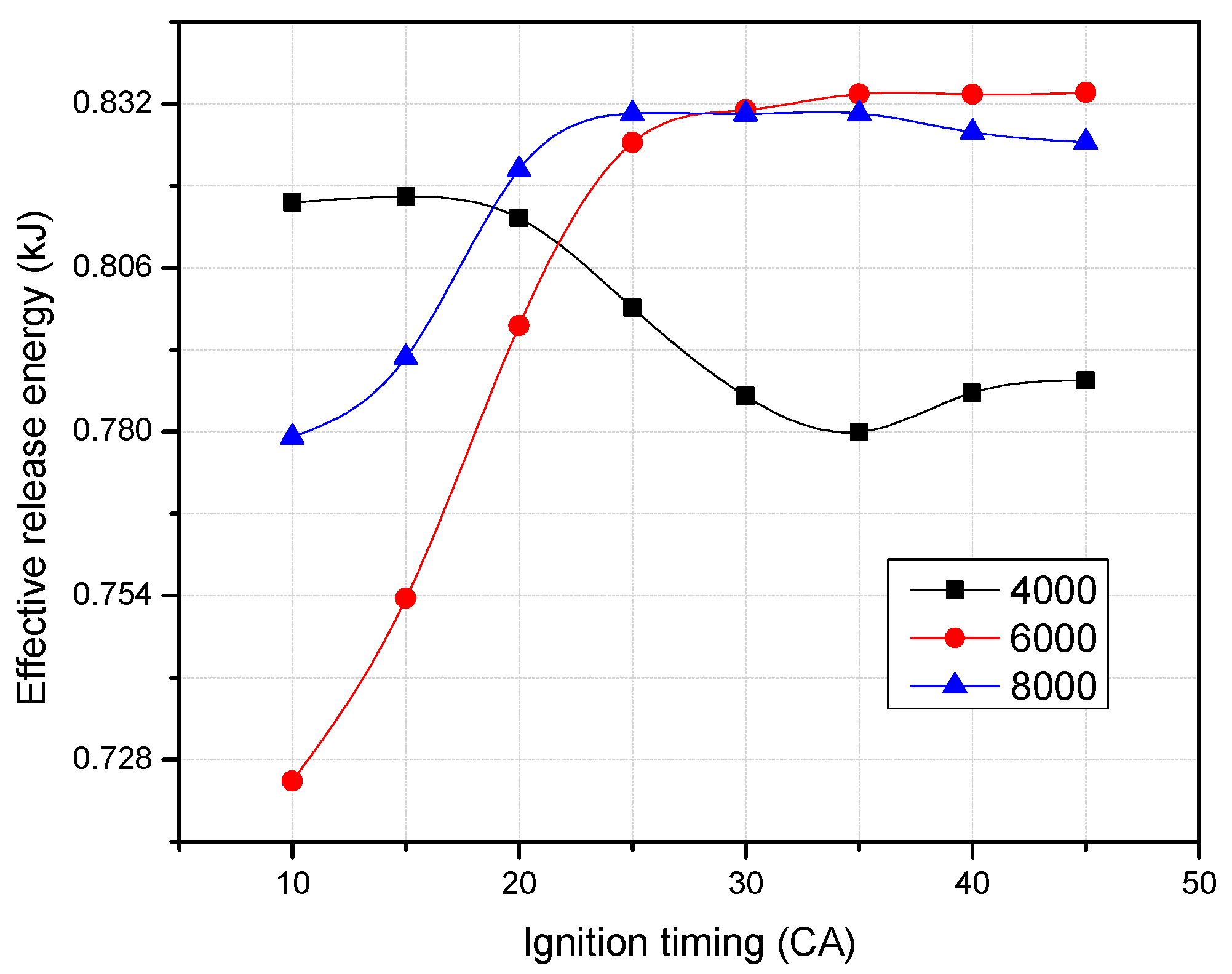
(1)

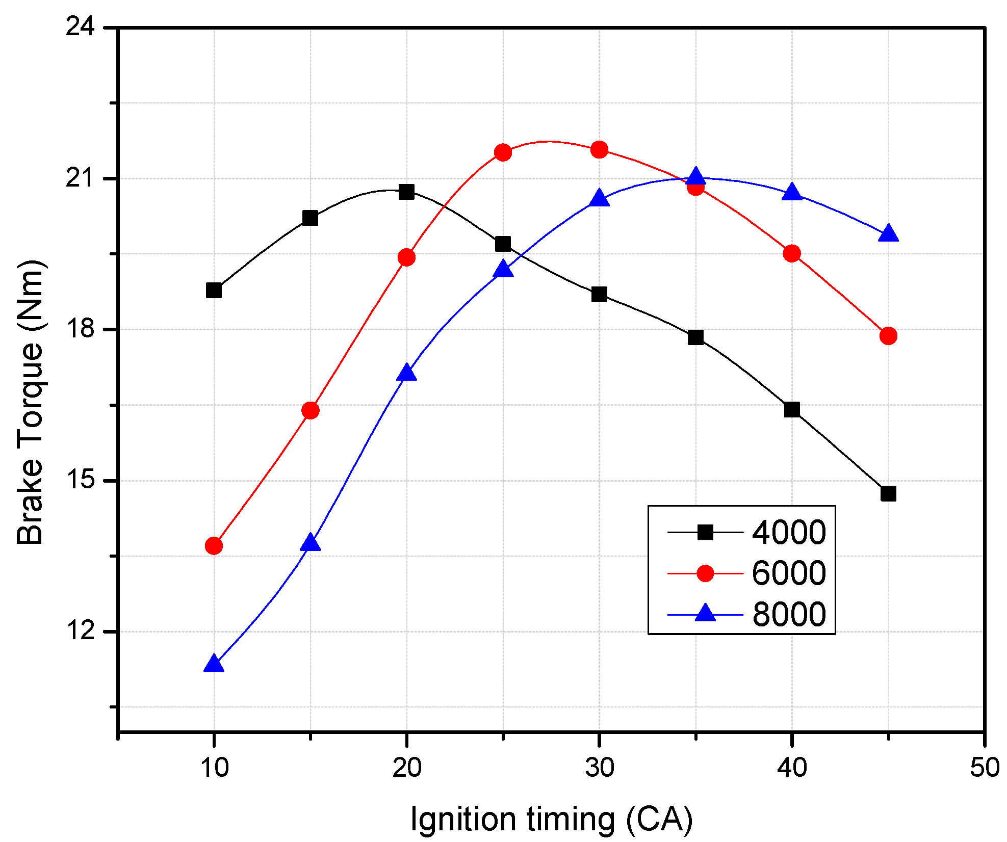
This paper denotes a major impact on residual gas ratio, effective release energy, performance, and characteristics of emissions resulting from ignition timing. The minimal residual gas proportion was 0.07% with a revolution speed of 8000 rpm and ignition timing of 10 °CA. Moreover, at 15 °CA of ignition timing, the highest effective release energy was 0.817 kJ at 4000 rpm, while at 8000 rpm, it was 0.8305 kJ at 25 °CA. At 6000 rpm, the highest braking torque was 21.57 Nm, while the minimal BSFC was 343.821 g/kWh.

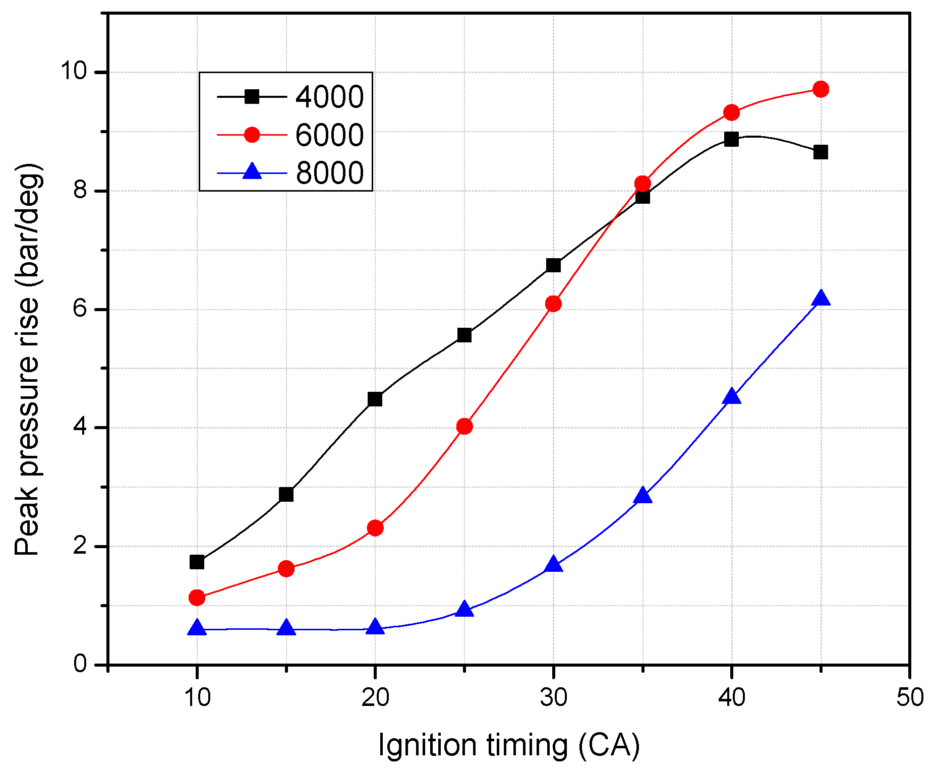
(2)

The peak firing temperature and peak pressure rise increase until achieving a maximum value when ignition timing increases. The peak firing pressure and peak pressure rise reached a maximum with a revolution of the engine at 6000 rpm and timing of ignition at 45 °CA. The maximum values are 108.36 bar and 9.71 bar/deg, respectively.

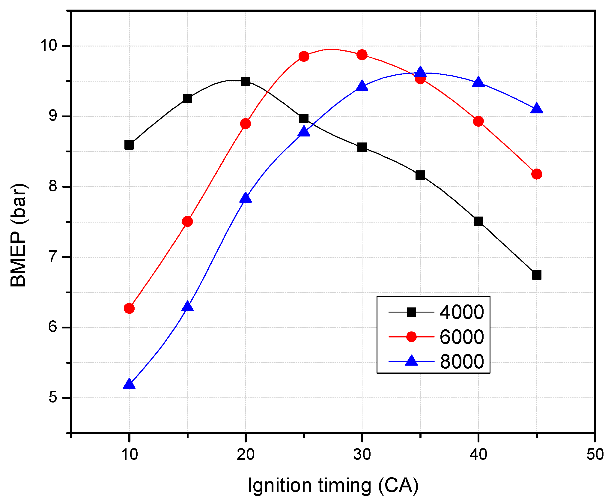
(3)

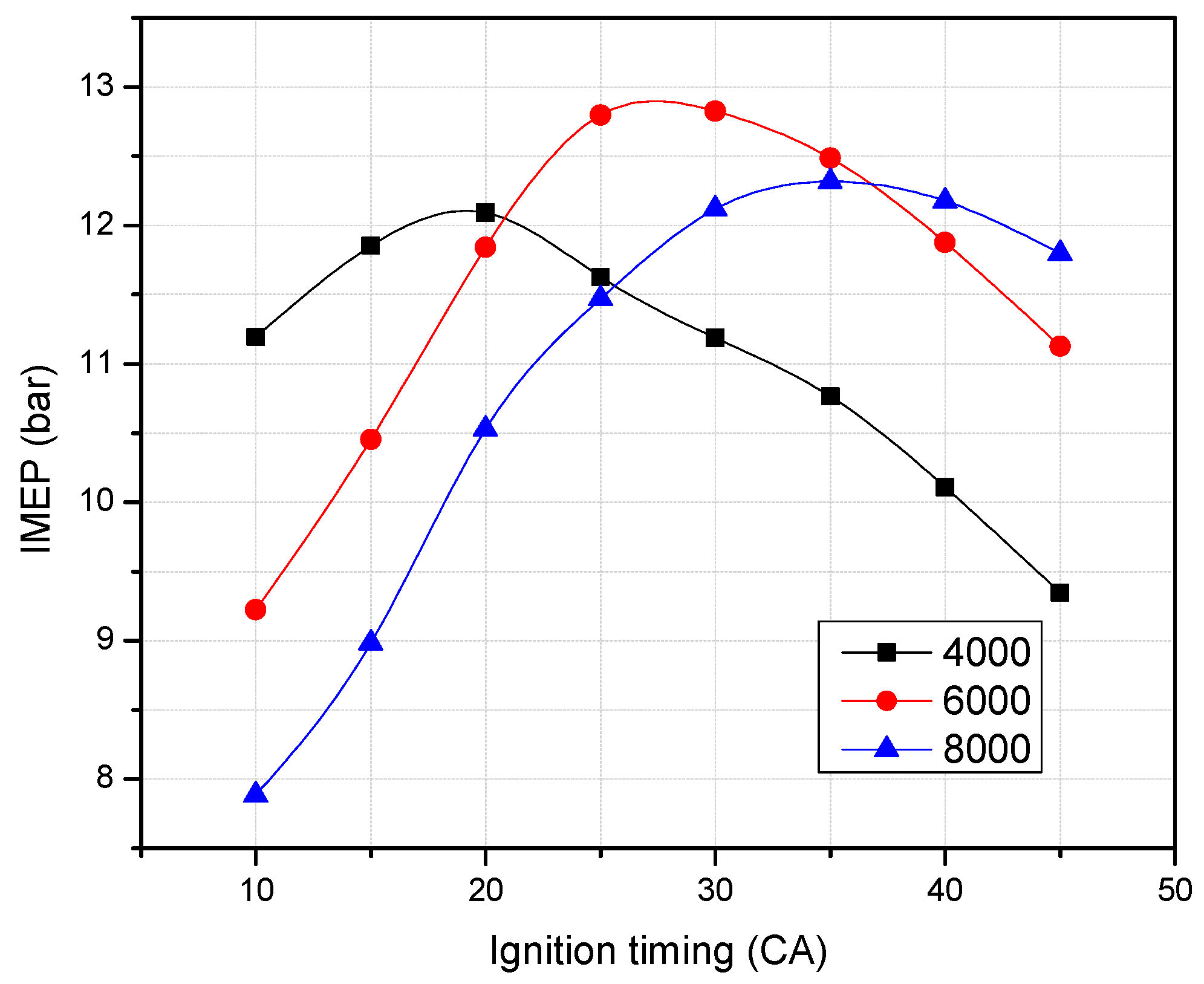
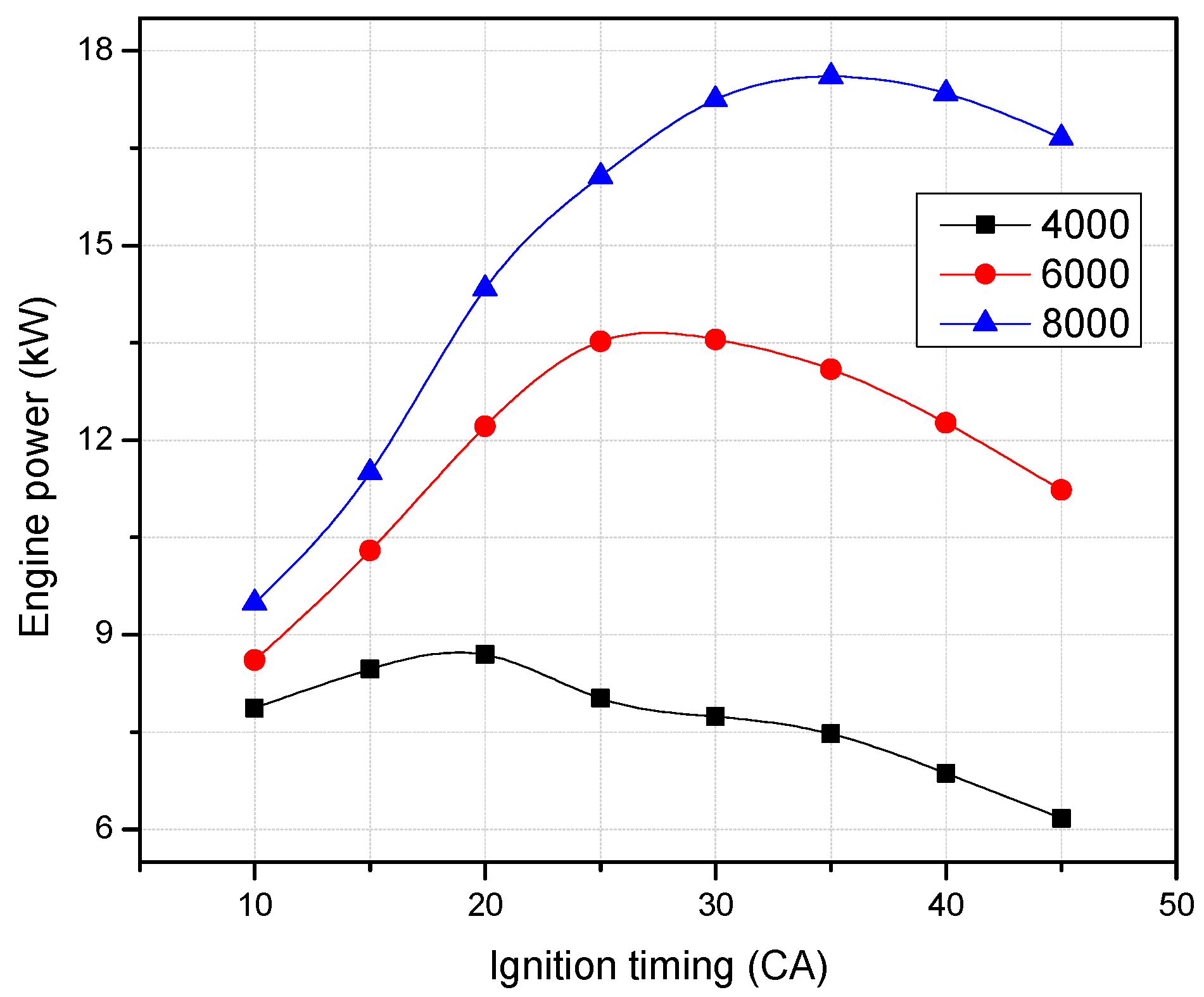
At various speeds of the engine, an optimum ignition timing value exists, and the engine will provide the best performance at that value. The optimum ignition timing was found to be 20 °CA at 4000 rpm in this analysis. The optimum ignition timing is 30 °CA and 35 °CA at 6000 rpm and 8000 rpm, respectively.

(4)

BMEP and IMEP rapidly increase to a peak. In the next stage, the trend reverses steadily. At each revolution speed, the optimal values of BMEP and IMEP at the same time as the ignition timing were reported.

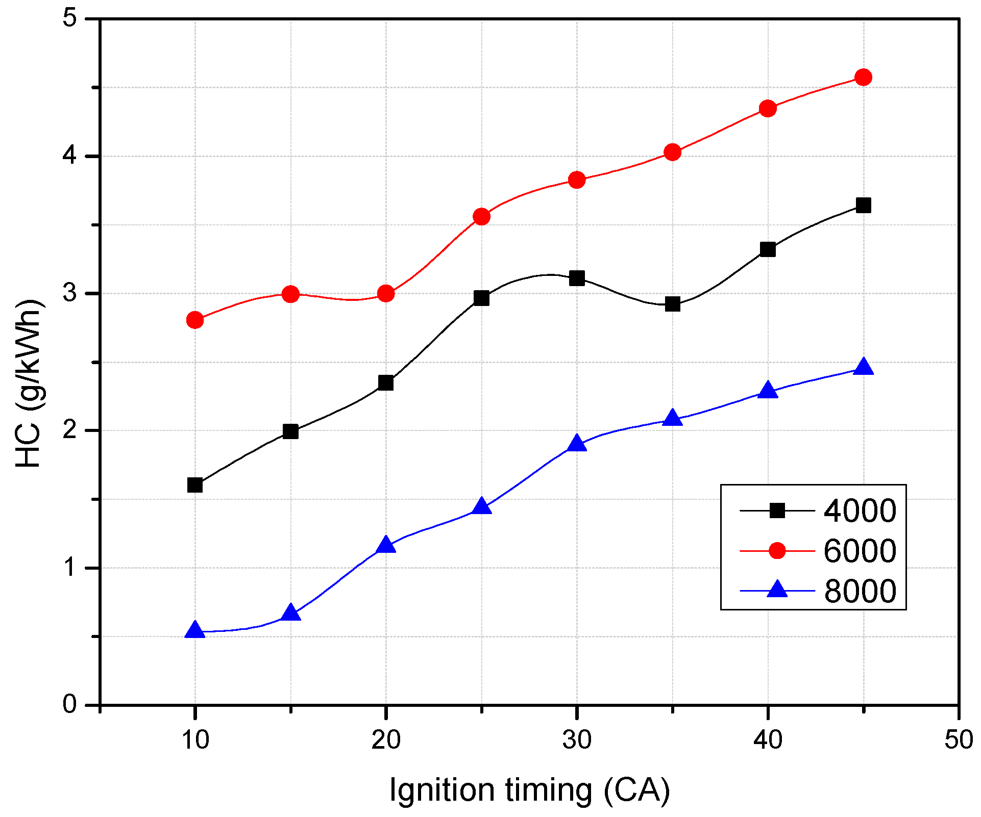
(5)

The residual gases play a key role in the characteristics of carbon monoxide emission. With increased residual gas, a reduction of the fresh air on the next charge will result. Hence, the growth of the residual gases directly increases carbon monoxide emission. The nitrogen oxide emission and HC emission increase with the advanced ignition timing.

References

- Muneer, T.; Asif, M.; Munawwar, S. Sustainable production of solar electricity with particular reference to the Indian economy. Renew. Sustain. Energy Rev. 2005, 9, 444–473. [Google Scholar] [CrossRef]
- Sayin, C.; Ertunc, H.M.; Hosoz, M.; Kilicaslan, I.; Canakci, M. Performance and exhaust emissions of a gasoline engine using artificial neural network. Appl. Therm. Eng. 2007, 27, 46–54. [Google Scholar] [CrossRef]
- Khoa, N.X.; Lim, O. Comparative Study of the Effective Release Energy, Residual Gas Fraction, and Emission Characteristics with Various Valve Port Diameter-Bore Ratios (VPD/B) of a Four-Stroke Spark Ignition Engine. Energies 2020, 13, 1330. [Google Scholar] [CrossRef] [Green Version]
- Khoa, N.X.; Lim, O. The Internal Residual Gas and Effective Release Energy of a Spark-Ignition Engine with Various Inlet Port–Bore Ratios and Full Load Condition. Energies 2021, 14, 3773. [Google Scholar] [CrossRef]
- Elfasakhany, A. Investigations on performance and pollutant emissions of spark-ignition engines fueled with n-butanol–, isobutanol–, ethanol–, methanol–, and acetone–gasoline blends: A comparative study. Renew. Sustain. Energy Rev. 2017, 71, 404–413. [Google Scholar] [CrossRef]
- Raviteja, S.; Kumar, G. Effect of hydrogen addition on the performance and emission parameters of an SI engine fueled with butanol blends at stoichiometric conditions. Int. J. Hydrogen Energy 2015, 40, 9563–9569. [Google Scholar] [CrossRef]
- Chan, S.H.; Zhu, J. Modelling of engine in-cylinder thermodynamics under high values of ignition retard. Int. J. Therm. Sci. 2001, 40, 94–103. [Google Scholar] [CrossRef]
- Soylu, S.; Van Gerpen, J. Development of empirically based burning rate sub-models for a natural gas engine. Energy Convers. Manag. 2004, 45, 467–481. [Google Scholar] [CrossRef]
- Hedfi, H.; Jedli, H.; Jbara, A.; Slimi, K. Modeling of a bioethanol combustion engine under different operating conditions. Energy Convers. Manag. 2014, 88, 808–820. [Google Scholar] [CrossRef]
- Li, J.; Gong, C.M.; Su, Y.; Dou, H.L.; Liu, X.J. Effect of injection and ignition timings on performance and emissions from a spark-ignition engine fueled with methanol. Fuel 2010, 89, 3919–3925. [Google Scholar] [CrossRef]
- Beatrice, C.; Belgiorno, G.; Di Blasio, G.; Mancaruso, E.; Sequino, L.; Vaglieco, B.M. Analysis of a Prototype High-Pressure “Hollow Cone Spray” Diesel Injector Performance in Optical and Metal Research Engines; SAE Technical Paper: Warrendale, PA, USA, 2017. [Google Scholar] [CrossRef]
- Vassallo, A.; Beatrice, C.; Di Blasio, G.; Belgiorno, G.; Avolio, G.; Pesce, F.C. The Key Role of Advanced, Flexible Fuel Injection Systems to Match the Future CO2 Targets in an Ultra-Light Mid-Size Diesel Engine; SAE Technical Paper: Warrendale, PA, USA, 2018. [Google Scholar] [CrossRef]
- Mohan, B.; Yang, W.; Kiang Chou, S. Fuel injection strategies for performance improvement and emissions reduction in compression ignition engines—A review. Renew. Sustain. Energy Rev. 2013, 28, 664–676. [Google Scholar] [CrossRef]
- Bae, C.; Kim, J. Alternative fuels for internal combustion engines. In Proceedings of the Combustion Institute, In Press. [CrossRef]
- Raheman, H.; Ghadge, S.V. Performance of diesel engine with biodiesel at varying compression ratio and ignition timing. Fuel 2008, 87, 2659–2666; [Google Scholar] [CrossRef]
- Xie, F.X.; Li, X.P.; Wang, X.C.; Su, Y.; Hong, W. Research on using EGR and ignition timing to control load of a spark-ignition engine fueled with methanol. Appl. Therm. Eng. 2013, 50, 1084–1091. [Google Scholar] [CrossRef]
- Anderson, J.E.; DiCicco, D.M.; Ginder, J.M.; Kramer, U.; Leone, T.G.; Raney-Pablo, H.E.; Wallington, T.J. High octane number ethanol–gasoline blends: Quantifying the potential benefits in the United States. Fuel 2012, 97, 585–594. [Google Scholar] [CrossRef]
- Sayin, C. The impact of varying spark timing at different octane numbers on the performance and emission characteristics in a gasoline engine. Fuel 2012, 97, 856–861. [Google Scholar] [CrossRef]
- Binjuwair, S.; Alkudsi, A. The effects of varying spark timing on the performance and emission characteristics of a gasoline engine: A study on Saudi Arabian RON91 and RON95. Fuel 2016, 180, 558–564. [Google Scholar] [CrossRef]
- Heywood, J.B. Internal Combustion Engine Fundamentals; McGraw-Hill Book Company: New York, NY, USA, 1988. [Google Scholar]
- Shi, W.; Yu, X.; Zhang, H.; Li, H. Effect of spark timing on combustion and emissions of a hydrogen direct injection stratified gasoline engine. Int. J. Hydrogen Energy 2017, 42, 5619–5626. [Google Scholar] [CrossRef]
- Elsemary, I.M.; Attia, A.A.; Elnagar, K.H.; Elsaleh, M.S. Spark timing effect on performance of gasoline engine fueled with mixture of hydrogen-gasoline. Int. J. Hydrogen Energy 2017, 42, 30813–30820. [Google Scholar] [CrossRef]
- Zhang, B.; Ji, C.; Wang, S. Combustion analysis and emissions characteristics of a hydrogen-blended methanol engine at various spark timings. Int. J. Hydrogen Energy 2015, 40, 4707–4716. [Google Scholar] [CrossRef]
- Yousufuddin, S.; Masood, M. Effect of ignition timing and compression ratio on the performance of a hydrogen-ethanol fueled engine. Int. J. Hydrogen Energy 2009, 34, 6945–6950. [Google Scholar] [CrossRef]
- Khoa, N.X.; Lim, O. The effects of combustion duration on residual gas, effective release energy, engine power and engine emissions characteristics of the motorcycle engine. Appl. Energy 2019, 248, 54–63. [Google Scholar] [CrossRef]
- Zareei, J.; Kakaee, A.H. Study and the effects of ignition timing on gasoline engine performance and emissions. Eur. Transp. Res. Rev. 2013, 5, 109–116. [Google Scholar] [CrossRef] [Green Version]