Optimizing Energy Consumption in Internal Transportation Using Dynamic Transportation Vehicles Assignment Model: Case Study in Printing Company

Abstract

Energy costs account for a significant proportion of total costs in production systems. Since energy is becoming an increasingly expensive resource, therefore, it is critical to consume it as efficiently as possible. Focusing on energy efficiency is also important in terms of reducing greenhouse gas (GHG) emissions and the effects of other pollutants on the environment. One of the possible ways for businesses to reduce energy consumption is to use available transportation means as efficiently as possible. In the operational phase, this can be achieved by reducing unnecessary transport, selecting the most efficient delivery routes, and by optimized assignment of available vehicles to transportation orders. We present in this article a novel dynamic assignment of transportation orders to fleet with energy minimization criterion in internal transport system of a printing company. The novelty of the proposed model is that, in contrast to most existing models, it can handle a heterogeneous fleet of human-operated and autonomous mobile robots (AMRs). The minimization of the energy consumption by transportation vehicles was modeled with reference to VDI 2198 standard. The need for such a model is justified by the fact that it better reflects a real production environment in many companies. The proposed optimization model was tested in simulation experiments imitating real production conditions in a large web printing house. The obtained results show that the proposed model allows for a significant reduction of energy consumption in internal transportation. The proposed model is general enough to be used in various companies with a heterogeneous fleet of internal transportation vehicles. In addition, the energy consumption factor VDI for AMRs has been determined, which can be useful in solving various problems related to energy optimization of internal transportation.

1. Introduction

Energy costs are becoming more of a burden for the private sector. For example, in 2021, the wholesale energy prices for businesses in Poland increased by over 40%, and many analysts predict that energy prices will continue to rise. Therefore, companies all over the world strive to reduce energy consumption to the maximum possible extent. The main way to achieve this was so far to reduce energy consumption in the core production processes. Currently, opportunities are being sought to reduce energy consumption in auxiliary processes, primarily logistic processes. Due to the recent development of technology and the prevalent logistics framework, the relevance of digitalized and autonomous transport is growing rapidly. Systems of automated guided vehicles (AGVs) often support internal transportation in manufacturing facilities and warehouses. Until recently, AGVs were the only option for automating internal transportation tasks; currently, however, AGVs are being challenged by more sophisticated, flexible, and cost-effective technology of autonomous mobile robots (AMRs). To this end, less expensive to operate autonomous or automated vehicles are being purchased, often as part of the implementation of a broader Industry 4.0 (or Logistics 4.0) concept. However, due to the high price of such vehicles and their technical limitations (e.g., maximum load capacity), it is not possible for many companies to replace traditional forklifts entirely. This means that transportation planners must deal with both types of vehicles and decide which type of vehicle to use to handle a given transportation order. However, in a real production environment, especially when transportation orders have high variability, it is almost impossible to make energy-efficient decisions. Therefore, decision supporting tools involving flexible energy optimization models are highly valuable.

Autonomous internal transportation vehicles are also very important in the energy transition in logistics addressing two main assumptions: (1) lowering energy consumption per kilometer-equivalent of goods transported-the energy reduction is achieved in AGVs, especially in the more modern AMRs by improving the efficiency of electric engines and batteries, as well as by introducing systems for recovering energy from braking or lowering the load, and (2) elimination a substantial proportion of emissions linked to transport and logistics-autonomous vehicles are powered by modern lithium batteries with very large charging cycles, which, as research indicates, significantly improves the total greenhouse gas emission indicator during their lifetime. In the future, increasing the use of autonomous vehicles in internal transport may become part of projects supported under national or transnational greening finance initiatives, as financial barriers hinder firm investments towards environmental innovations, especially in SME sector [1]. The assumption presented in Green Economy Transition 2021–2025 document published by the European Bank for Reconstruction and Development clearly mentions sustainable connectivity, including logistics systems, as one of the key thematic areas that should be accelerated within greening the finance system.

Currently, however, due to the high prices of autonomous vehicles as well as their technical limitations (e.g., maximum load capacity, adequate floor area), it is not possible for many companies to replace traditional forklifts entirely. This means that transportation planners must deal with both types of vehicles and decide which type of a vehicle to use to handle a given transportation order. However, in a real production environment, especially when transportation orders are highly variable, it is almost impossible for humans to make energy-efficient decisions. Therefore, decision supporting tools involving flexible energy optimization models are highly valuable.

To meet the energy saving challenges in current logistic processes, we propose in this paper a novel dynamic optimization model which aims to minimize the energy consumption in the internal transportation system of a production plant. The proposed model reflects real-time conditions by considering constraints on the capacity of transportation vehicles, constraints on the transportation network (restricted areas), priorities of transportation orders, and all required safety requirements. The proposed here approach differs from approaches to the optimization of internal transportation described in the literature (see Section 2) in that it is focused on minimization of energy consumption and it considers a heterogeneous fleet of transportation vehicles including modern, energy-efficient autonomous mobile robots (AMR) and traditional human-operated electric forklifts. Another novelty described in this paper is the accurate measurement of energy consumption in AMR according to the VDI (short for Verein Deutscher Ingenieure, the association of German engineers) standard, commonly used in Europe (especially in German-speaking countries), which allows for a reliable comparison of energy consumption between AMRs and traditional electric forklifts, and which can be useful in solving various problems related to energy optimization of internal transportation. The usefulness of the proposed model is verified in a case study of a web printing company where energy efficient and reliable transportation is increasingly desirable. The company uses a heterogeneous fleet of transportation vehicles covering human-operated forklifts and a few quite recently purchased AMRs. The results of the simulation study and tests performed in conditions close to real production processes (characterized by a large variety of products and fluctuating ordering pattern) indicate great efficiency of the proposed model in reducing the total energy consumption by the internal transportation processes. The proposed model is very flexible, and therefore can be straightforwardly, or with few modifications, used in various companies with a heterogeneous fleet of internal transportation vehicles.

The rest of the paper is organized as follows. Since energy consumption issues are of our primary concern, we present in Section 2 an overview of the literature on energy consumption in internal transportation systems, and we discuss the literature on routing and scheduling of transportation vehicles. The proposed approach for dynamic assignment of transportation orders to heterogeneous fleet in the internal transportation system of a production plant is presented in Section 3. Section 4 is devoted to the considered case study. The obtained results are discussed in Section 5. The paper ends with concluding remarks.

2. Literature Overview Related to Internal Transportation Vehicles Assignment and Scheduling Problem with Energy Consumption Criterion

A comprehensive analysis of the transport literature has shown that relatively little scientific work has so far been devoted to the problem of energy saving in internal transportation. Moreover, the existing literature on the subject concerns almost exclusively AGVs and can be generally divided into two groups: the literature related to the technical operation and control of AGVs, and the literature related to the optimization of AGVs allocation to orders, charging their batteries, and routing optimization. Below, we present a brief overview of the available related literature.

2.1. Energy Consumption Models

The technical aspects of energy consumption were presented by Scholz et al. [2]. In their work they analyzed the impact of load profiles on the energy consumption of AGVs, conveyor belts and forklift trucks using a specially constructed measurement environment with an embedded vision system, among others. The energy efficiency of alternative assets was measured, simulated, and characterized by energy performance indicators (EPI).

A detailed model of energy consumption by AGVs was presented by Meißner et al. [3] They analyzed the energy consumption in terms of speed, payload, and lifting operation, and showed that autonomous vehicles are the most energy-efficient when a transport process is performed at maximum speed. They observed as well that the energy demand decreases when the operating temperature of the vehicles increases.

Carli et al. [4] proposed an optimization model that aimed to identify an optimal control strategy for the battery charging of a fleet of electric mobile material-handling equipment (MHE), e.g., autonomous vehicles. Their model enabled them to jointly evaluate the job scheduling and the energy consumption profile of MHE in picking processes.

However, none of the above works answers the question which reference value should be used as the energy consumption factor for automated vehicles and none of them is directly related to AMRs, which are increasingly often becoming part of the internal transportation fleet in many companies. Hence, the need for models that can take AMRs into account, and in order to obtain reliable results, an energy consumption (VDI standard compliant) indicator for AMRs must be determined.

2.2. Operational Management of AGVs

Scientific works related to the implementation of AGVs are devoted mainly to various methods for optimizing AVGs operations in, e.g., manufacturing, distribution, transportation, and transshipment. As energy saving goals are rarely considered, this section will present the most important works related to the operational management of AGVs in general and the few that also analyzed energy consumption.

The problem of routing and scheduling of transportation vehicles can be divided into two subproblems [5]: the vehicle-dispatching problem, which relies on assigning tasks to vehicles and sequencing these tasks for each vehicle, and the vehicle-routing problem where optimal, with respect to some criteria, routes are searched for a given sequence of orders, in particular, arrival and departure times are determined for all vehicles. The main criteria subject to optimization considered in the literature include [6]:

• Maximization of transportation system capacity;
• Minimization of makespan (the time elapsed between the start and finish of a sequence of jobs or tasks);
• Minimization of vehicles total travel times and distance;
• Minimization total transportation cost;
• Minimization of AGVs waiting time for loading;
• Minimization of the number of required vehicles;
• Minimization of tardiness rate;
• Energy consumption.

The optimization is usually performed under various constraints. To reflect a real-life manufacturing environment, the constraints should include limited vehicles load, material loading-unloading times or tasks specificity. The more constraints are imposed, the more complex the problem is and more sophisticated tools must be used.

The two subproblems described above can be solved separately or simultaneously. using both exact methods, heuristics, and metaheuristics [5]. Exact methods always solve an optimization problem to optimality, however, because of the NP-hard nature of the routing and scheduling problems [7], heuristic and metaheuristic approaches seem to be more suitable, especially when dealing with more complex and large-scale problems.

2.2.1. Exact Approaches

Meersmans and Wagelmans [8] developed a branch and bound (B&B) algorithm to solve the problem of integrated scheduling of various types of handling equipment at an automated container terminal. The objective was to minimize the makespan of the schedule. This integrated approach did not consider limited space for AGVs waiting to be loaded/unloaded at the cranes.

Nishi et al. [9] addressed a bilevel decomposition method for solving the simultaneous scheduling and conflict-free routing problems for AGVs. The overall objective was to minimize the total weighted tardiness of the set of jobs.

Desaulniers et al. [10] presented an approach to obtain the exact solution to the problem of the simultaneous dispatching and conflict-free routing of AGVs carrying out material handling tasks in a flexible manufacturing system. The objective was to minimize the costs related to the production delays. Their approach combined a greedy search heuristic used to find a feasible solution, column generation, and a branch and cut procedure. The performance of the proposed approach was limited by the search heuristic, which performed poorly for a larger congestion.

Rashidi and Tsang [11] proposed a polynomial time complexity NSA+ algorithm, which extended the standard network simplex algorithm (NSA), for scheduling AGVs in container terminals. The objective was to minimize the cost of flow. Although the algorithm turned out to be efficient, it can work only for problems of limited size. To solve problems that go beyond the abilities of NSA+ or when the time available for computation is too short, Rashidi and Tsang designed and implemented an incomplete greedy vehicle search (GVS) algorithm.

2.2.2. Heuristic and Metaheuristic Approach

A hybrid genetic algorithm was proposed by Zhang et al. [12] to solve the vehicles dispatching problem for JIT distribution in numerical control (NC) workshop. The algorithm combined a greedy sweep matrix algorithm designed to allocate the distribution mission for vehicles with an improved genetic algorithm aimed to solve the best distribution order for each vehicle.

Li et al. [13] proposed an improved harmony search algorithm with an effective discrete encoding scheme of harmony, a new initialization method for harmony memory based on opposition-based learning strategy, a dynamic harmony memory considering rate parameter, and a local search strategy. They evaluated the proposed approach through three cases from the real-world manufacturing system for producing the back cover of smartphone.

An ant-colony algorithm was proposed by Saidi-Mehrabad et al. [14] to simultaneously solve a job shop scheduling problem considering the transportation times of the jobs from one machine to another and the conflict-free routing problem. The objective was to minimize the makespan.

Zheng et al. [15] proposed a heuristic algorithm based on tabu search to get the optimal or near to optimal solution to the large-size problem of simultaneous scheduling of machines and AGVs in a flexible manufacturing system (FMS). The objective in the developed mixed-integer programming problem was to minimize the makespan.

Zhang and Li [16] developed an improved particle swarm optimization algorithm with the characteristics of main particles and nested particles to solve the resources optimization problem of AGV-served manufacturing systems driven by multivarieties and small-batch production orders. The objective was to minimize the makespan of jobs from raw material storage to finished parts storage through multistage processes.

Abdelmaguid et al. [17] proposed a new hybrid genetic algorithm/heuristic coding scheme for solving the problem composed of two interrelated decision problems: the scheduling of machines, and the scheduling of AGVs in flexible manufacturing systems (FMS). The objective was to minimize the makespan.

A similar problem with AGVs operating in FMS was solved by Reddy and Rao [18] using a hybrid multiobjective genetic algorithm. The objective function this time was a combination of makespan, mean flowtime, and mean tardiness. The algorithm performed similarly to the one proposed by Abdelmaguid et al. [17] when only the makespan criterion was considered.

Yet another approach for developing simultaneous schedules for machines and AGVs in FMS has been proposed by Erol et al. [19]. They used a multiagent system in which machines and AGV playing a role of scheduler agents interacted with a manager agent, staff agent, and operations agents. Such an approach was tested on the problems first described by Bilge and Ulusoy [20].

Zou et al. [21] proposed a discrete bee colony algorithm to solve the problem of AGVs scheduling in a linear manufacturing workshop in which total travel distance and deviation of waiting time by distribution points (call cells) were considered.

Xiao et al. [22] adopted a multiattribute task scheduling principle, considered the traffic subsystem and the processing subsystem separately, and proposed a strategy of avoiding deadlock.

Guang et al. [23] developed a variable neighborhood niche genetic algorithm (VNS/NGA) by studying and analyzing the existing path design methods. Xia et al. [24] built a model based on the viewable link map in a static environment and used the GA to carry out path planning and improvement on AGV, which can quickly search for the optimal path of AGV.

Song et al. [25] put forward an optimization plan for the distribution system by using the industrial engineering method and simulated the logistics distribution system of the engine assembly line. Based on the characteristics of simulation analysis and logistics distribution system, Wang et al. [26], combined with a heuristic algorithm to obtain a solution that is suitable for the actual needs of the assembly line, at the same time, they proposed a vehicle dynamic scheduling method through adjusting the control strategy and dynamic simulation of decision parameters.

Liang et al. [27] provided a hybrid algorithm combining the Dijkstra algorithm and Hungarian algorithm to obtain the shortest path matrix of no-load and load firstly, and then to get the assignment of AGVs to the transport tasks according to the urgent task set.

Corréa et al. [28] proposed a hybrid method to solve the problem of dispatching and conflict-free routing of AGVs in a flexible manufacturing system (FMS). The hybrid decomposition method presented therein allowed to solve instances with up to six AGVs. A hybrid algorithm for solving the multitask assignment and routing optimization problem of AGVs was also proposed by Fazlollahtabar and Hassanli [29].

Zhou and Schen [30] considered a bi-criterial problem of AGVs scheduling in an assembly-line. The goal functions were defined as weighted tardiness for completing all pick and delivery requests and the total energy consumption associated with the operation of AGVs. A tabu search algorithm was used to initialize solutions in a multiobjective particle swarm optimization to solve the problem. In the Pareto analysis, they showed that the energy saving criterion was in a strong conflict with total tardiness.

Angeloudis and Bell [31] considered the problem of developing schedules for AGVs operating in a container terminal, in which tasks duration were uncertain. They modeled the uncertainty using intervals and used a binary integer programming model to solve the problem.

Bányai et al. [32] proposed an optimization model of logistics resources in a matrix production system with in-plant supply based on AGVs. The optimization was performed in two phases: the demands clustering phase and the energy consumption minimization phase. In the first phase, the available supply-demands were clustered based on time frame related objective function (clustering step), and next, the clusters were scheduled (routing and scheduling phase). In the second phase, the energy consumption of AGVs was minimized during the whole in-plant supply process including scheduled routes (extended optimization) and new supply-demands (real-time optimization). Bányai et al. used the black hole algorithm for clustering of supply-demand and flower-pollination-based algorithm for routing and rerouting. Their model enabled as well to calculate greenhouse gas emission of the electricity used by AGVs.

2.2.3. Simulation Approach

Singh et al. [33] proposed dedicated dispatching rules for one and two AGVs. The performance of the rules was evaluated in simulation by monitoring parameters reflecting efficiency and uniformity of material distribution in a flowshop.

Monte Carlo simulation model for scheduling AGVs in a flexible automated manufacturing system was proposed by Fazlollahtabar et al. [34]. They considered the waiting time, transportation time and failure time for the vehicles, and processing time for the machines.

2.3. Comparison of Internal Transport Models

The literature review shows that scientific works related to the optimization of internal transportation are devoted mainly to optimization of AVGs operation concerning makespan, total tardiness or waiting time. The proposed in this paper approach focuses on a highly up-to-date problem, i.e., minimization of energy consumption. The novelty of the proposed approach is that it considers a heterogeneous fleet of transportation vehicles, and therefore better reflects real conditions in many production companies. The proposed optimization model considers various additional constraints, which mean the model is general enough to be used in production companies from various industries.

The comparison of the proposed approach with other methodologies is summarized in Table 1.

Table 1. Summary of selected publications on AGV scheduling problem.

Reference	Objective Function	Approach	Problem Specificity	Energy Saving
Meersmans and Wagelmans [8]	Makespan	Exact algorithm		No
Nishi et al. [9]	Total tardiness of tasks	Exact algorithm		No
Desaulniers et al. [10]	Production delay costs	Exact algorithm		No
Rashidi and Tsang [11]	Flow cost	Exact algorithm		No
Zhang et al. [12]	Flow cost + delay cost	Metaheuristic		No
Saidi-Mehrabad et al. [14]	Makespan	Metaheuristic		No
Zheng et al. [15]	Makespan	Metaheuristic		No
Zhang and Li [16]	Makespan	Metaheuristic		No
Abdelmaguid et al. [17]	Makespan	Metaheuristic		No
Reddy and Rao [18]	Makespan, mean flowtime, and mean tardiness.	Metaheuristic		No
Zou et al. [21]	Total travel distance	Metaheuristic	Vehicle waiting time	Yes
Xiao et al. [12]	Empty travel distance	Heuristic	Tasks Urgency	No
Xia et al. [24]	Travel distance	Metaheuristic		No
Liang et al. [27]	Travel distance	Exact algorithm	Task Urgency	No
Zhou and Schen [30]	Tardiness rate, energy consumption	Metaheuristic		Yes
Angeloudis and Bell [31]	Fleet utilization, travelled distance, vehicle productivity	Heuristic	Uncertainty of task duration	No
Fazlollahtabar et al. [34]	Vehicle waiting time, transportation time	Simulation	Vehicle failure time	No
Bányai et al. [32]	Energy consumption	Clustering and heuristic	Clustering of supply demand	Yes
Proposed Approach	Vehicle energy consumption based on VDI standard	A simulation model based on Dijkstra and Clarke Wright algorithm	A heterogeneous fleet of vehicles	Yes

3. Proposed Approach to Assignment of Transportation Orders to Heterogeneous Fleet in Internal Transport System with Energy Minimization Criterion

3.1. Problem Description

The problem of assignment of transportation orders to a fleet of heterogeneous vehicles is a complex decision problem. It belongs to the class of combinatorial optimization problems, which are considered by some literature as optimization problems dealing with graph structures. In the approach proposed here, we assume that the heterogeneous fleet may consist of transportation vehicles that differ in their maximum capacity, physical weight parameters, operational speed, energy consumption factor, and the type of control (manual or autonomous). In addition, we consider the following constraints, which makes the problem even more complex:

• Transportation vehicles have different sizes, which limits their ability to enter and move within certain areas of the internal transportation network (restricted areas),
• Materials (semifinished and finished products) can only be transported by specific types of transportation vehicles,
• The number of available transportation vehicles and the number of transportation orders can change dynamically during the scheduling period.

The objective of the proposed dynamic approach is to minimize the total energy consumption by the transportation fleet through optimal assignment of transportation orders to transportation vehicles, within the above-given constraints.

The model is designed to work in a real production environment, so it should reflect real conditions as much as possible. The real conditions can be considered in the assignment problem in two ways: by increasing the complexity of the base model or by applying a data-driven approach. The operational character of the real-life processes makes that the first approach may be impractical due to excessive computing time; therefore, we use the data-driven approach. Generally, two main stages can be distinguished in our model (see Figure 1): the preprocessing stage and the optimization stage. In the preprocessing stage, we determine the actual state of the system and we process and prepare data required for the second stage. In the second stage, the assignment of transportation orders to transportation vehicles is optimized based on data obtained in the first stage.

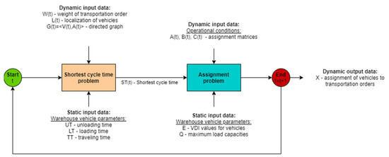
Figure 1. Proposed approach for dynamic assignment of transportation orders to heterogeneous of transportation vehicles.

3.2. Model Input Data

Model sets definition:

• $T=\left\{t:t=1,2,\dots ,\left|T\right|\right\}$—the set of timestamps.
• $R=\left\{r:r=1,2,\dots ,\left|R\right|\right\}$—the set of types of logistic units.
• $K=\left\{k:k=1,2,\dots ,\left|K\right|\right\}$—the set of types of transportation vehicles.
• $W=\left\{w:w=1,2,\dots ,\left|W\right|\right\}$—the set of nodes (e.g., intersections of paths) of the internal transportation network.
• $M^{\left(r\right)}$—the set of transportation orders for every r-th type of transportation vehicle.
• $M={{\displaystyle \cup }}_{r\in R}{M}^{\left(r\right)}=\left\{j:j=1,2,\dots ,m\right\}$—the set of transportation orders to be completed by transportation vehicles.
• $N^{\left(k\right)}$–the set of transportation vehicles of k-th type.
• $N={{\displaystyle \cup }}_{k\in K}{N}^{\left(k\right)}=\left\{i:i=1,2\dots ,n\right\}$—the set of all transportation vehicles that can be used in the internal transportation system (we assume that each index in $N$ corresponds to a certain transportation vehicle).

Input model parameters:

• $UT=\left[u{t}_j\right]$—the vector of unloading times; $u{t}_j$ is the unloading time of the j-th transportation order.
• $LT=\left[l{t}_j\right]$—the vector of loading times; $l{t}_j$ is the loading time of the j-th transportation order.
• $TT=\left[t{t}_{od}\right]$—the matrix of traveling times; $t{t}_{od}$ is the traveling time between the pair of nodes $\left(o,d\right)$ corresponding to origin ($o$) and destiny ($d$) points.
• $D=\left[d_j\right]$—the vector of weights; $d_j$ is the weight of the j-th transportation order.
• $A=\left[a_{ik}\right]$—the matrix of assignment data; $a_{ik}=1$ if the i-th transportation vehicle is of type k, otherwise $a_{ik}=0$.
• $B=\left[b_{rj}\right]$—the matrix of assignment data; $b_{rj}=1$ if a logistics unit of type r can handle the j-th transportation order, otherwise $b_{rj}=0$.
• $C=\left[c_{rk}\right]$—the matrix of assignment data; $c_{rk}=1$ if a logistics unit of type r can be operated by a transportation vehicle of type k, otherwise $c_{rk}=0$.
• $E=\left[e_i\right]$—the vector of energy consumption factors expressed by the VDI value; $e_i$ is the energy consumption factor of the i-th transportation vehicle.
• $Q=\left[q_i\right]$—the vector of maximum load capacities; $q_i$ is the maximum load capacity of the i-th transportation vehicle.

Indirect model parameters:

• $ST=\left[s{t}_{ij}\right]$—the matrix of the shortest time cycles; $s{t}_{ij}$ is the shortest time cycle between the current localization (the current localization of a transportation vehicle is obtained from the real time localization system (RTLS)) of the i-th transportation vehicle at the t-th timestamp and the destination point of the j-th transportation order. Remark: this data is obtained in the preprocessing stage at every t-th timestamp; the data include travelling time from the current localization, loading time for pallet pickup at the origin point for the j-th transportation order, travel time from the origin point to the destination point for the j-th transportation order, and finally, the pallet unloading time at the destiny point for the j-th transportation order.

Note: The number of elements in the sets $R,K,D,M,M^{\left(r\right)},N,N^{\left(k\right)}$ depends on the current timestamp, but for simplicity of the notation, and due to the iterative nature of the proposed procedure, the time index will be hereinafter omitted.

3.3. Shortest Time Cycle Problem

Let us consider a directed graph $G=⟨V,A⟩$ that represents the transportation network at the t-th timestamp (let us recall that the timestamp index is omitted due to the reasons given above). The set $V$ of graph vertices represents all nodes of the transportation network, all source points of transportation orders, and current localizations of transportation vehicles, i.e., $V=W{{\displaystyle \cup }}^{}M{{\displaystyle \cup }}^{}N$. The set of directed edges $A=\left\{\left(o,d\right):o,d\in V\right\}\subseteq V\times V$ represents the links between vertices of the graph. Given the function $\zeta :V\times V\to \left\{0,1\right\}$, it holds that $\zeta \left(o,d\right)=1$, if $\left(o,d\right)\in A$ (there is a direct link between the pair of nodes $\left(o,d\right)$), otherwise $\zeta \left(o,d\right)=0$. Note: the input data such as $u{t}_j$, $l{t}_j,j\in M$ must be extended to $ut{\prime }_o$, $lt{\prime }_o,o\in V$. It is assumed that $ut{\prime }_o=0$, $lt{\prime }_o=0$ for all $o\in W{{\displaystyle \cup }}^{}N$.

The aim of the proposed model is to determine the shortest time cycle from the origin point: $\left\{org\right\}\in V$ to the destiny point: $\left\{des\right\}\in V$ for transportation vehicles at the t-th timestamp. The model is formulated as follows:

Decision variables:

• ${\mathit{X}}^{sp}=\left[x_{od}^{sp}\right]$—binary variables indicating if the arc between the nodes $o$ and $d$ belongs to the solution (is in the solution path), $x_{od}^{sp}=1$ if arc between the nodes $o$ and $d$ belongs to the solution, otherwise $x_{od}^{sp}=0$.

Objective function:

$$\begin{array}{cc}F:& \underset{x_{od}^{sp}}{min}\left[{\sum }_{\left(o,d\right)\in A}^{}{x}_{od}^{sp}·t{t}_{od}+{\sum }_{o\in V}\left({\sum }_{d\in V}{x}_{od}^{sp}·\left(lt{\prime }_o+ut{\prime }_o\right)\right)\right]\end{array}.$$

(1)

and the flow constraint:

$${\sum }_{\left\{o:\left(o,d\right)\in A\right\}}{x}_{od}^{Sp}-{\sum }_{\left\{d:\left(o,d\right)\in A\right\}}{x}_{od}^{Sp}=\{\begin{array}{c}\begin{array}{cc}1,& ifo=\left\{org\right\}\end{array}\\ \begin{array}{cc}-1,& ifd=\{des\end{array}\}\\ \begin{array}{cc}0,& otherwise\end{array}\end{array},$$

(2)

Nature of decision variables constraints:

$$\begin{array}{cc}{x}_{od}^{sp}\in \left\{0,1\right\},& \forall \left(o,d\right)\in A\end{array}.$$

(3)

3.4. Assignment Problem

The problem of transportation orders management and scheduling in the company’s internal transportation system can be formulated as a mixed-integer linear programming problem. The objective is to minimize the energy consumption of transportation vehicles. The model is formulated as follows:

Decision variables (assignment matrix):

• $\mathit{X}=\left[x_{ij}\right]$—binary variables indicating if the i-th transportation vehicle executes the j-th transportation order, $x_{ij}=1$ if the i-th transportation vehicle executes the j-th transportation order, otherwise $x_{ij}=0$.

Objective function:

Function $F$ minimizes the total energy consumption of the transportation fleet through an effective allocation of vehicles to transportation orders. This is achieved by reducing the distance travelled:

$$\begin{array}{cc}F:& \underset{x_{ij}}{\mathit{min}}{\sum }_{i\in N}{e}_i{\sum }_{j\in M}\left(x_{ij}·s{t}_{ij}\right)\end{array}.$$

(4)

Assignment constraints:

$$\begin{array}{cc}{\sum }_{i\in N}{x}_{ij}\le 1,& \forall j\in M\end{array},$$

(5)

$$\begin{array}{cc}{\sum }_{j\in M}{x}_{ij}=1,& \forall i\in N\end{array},$$

(6)

The first constraint ensures that each transportation order is serviced by at most one vehicle, and the second constraint ensures that each transportation vehicle is assigned to exactly one transportation order.

Capacity constraints:

$$\begin{array}{cc}{\sum }_{j\in M}{d}_j·x_{ij}\le q_i,& \forall i\in N\end{array}.$$

(7)

Constraint ensuring that each transportation order is assigned to a proper type of transportation vehicle:

$$x_{ij}\le \begin{array}{cc}{a}_{ik}·b_{rj}·c_{rk},& \forall i\in N,\forall j\in M,\forall r\in R,\forall k\in K\end{array}.$$

(8)

Formula (8) guarantees that the variable $x_{ij}$ for all i and j, is equal to 1 only if all technical condition described by assignment matrices A, B and C are satisfied (the conjunction of assignment data in A, B and C matrix must equal 1). Nature of decision variables constraints:

$$\begin{array}{cc}{x}_{ij}\in \left\{0,1\right\},& \forall i\in N, \forall j\in M\end{array}.$$

(9)

3.5. Modeling and Simulation Process

Our proposed approach to optimizing the energy consumption within an internal transportation system was verified by a simulation-based study. A systematic procedure for modeling and simulation process of internal transportation is briefly described in Figure 2.

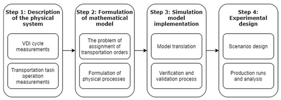
Figure 2. Main steps in modelling the assignment of transportation orders to heterogeneous fleet in internal transport system with energy minimization criterion.

The first step, description of the physical system, mainly focuses on collecting the data about major tasks and objects in internal transportation processes (more details in Section 3.2 and Section 3.3). The optimization model assumes that energy minimization is realized by assigning the vehicles with the smallest VDI value, so the appropriate measurement was done (more details in Section 4.1). The second stage is to build a mathematical model for the order assignment process and define other mathematical expressions describing the system features (more details in Section 3.4 and Section 3.5). Step 3 is the simulation model translation and implementation. During this step, the logic of the optimization model and simulation model is translated into a simulation program (see more in Appendix A). An important step is the verification and validation process. In our approach only the process of assignment of transportation orders to the heterogeneous fleet in the internal transport system will be changed, so the rest components of the simulation system are verified. The last step was experimental design and analysis (see more details in Section 5).

The simulation model was designed on hybrid approach: it combines the classical components of simulation model (e.g., system entities, input variables, performance measurement, or functional relationships) and the optimization processes based on Dijkstra and Clarke–Wright algorithm. The optimization proses in the simulation model was used to dynamic computing the shortest path between the transportation vehicles localization and origin/destiny of transportation orders in the system. Logic and functional relationships of the simulation model were destined on mathematical model described in previous section.

4. Case Study of Internal Transportation System in Web Printing Company

The proposed approach to optimize the energy consumption within an internal transportation system was tested using a real-world example—the system of managing the requests for deliveries of raw materials, finished products, and wastes in a large web printing company. To test the proposed approach, we have created the simulation model developed the specialized software written in C# programming language (for more details on software implementation see Appendix A). Input data for simulation model based on real-life data and information describing the physical components of the internal transportation of the printing company. In our approach we made two main assumptions: we are considering the human-operated and the autonomous transportation vehicles and simultaneously and the managing criterion in the internal transportation system is the energy consumption by transportation vehicles represented by VDI cycle.

4.1. Simulation Data Parameters: Characteristics of Human-Operated and Autonomous Transportation Vehicles in Company

The design simulation model considers the following two basic types of battery electric transportation vehicles (see Table 2 and Figure 3), which handle most of the internal transportation system of the considered printing company.

Table 2. Technical parameters of transportation vehicles.

Parameter/Vehicle Type	MiR1000	Toyota BT LPE200	YALE MP20XFBW
Load capacity [kg]	1000	2000	2000
Lifting height [m]	0.05	0.2	0.12
Loading method	Loading dock	Floor	Floor
Control	Autonomous	Operator	Operator
Velocity [km/h]	1.2	7.5	6
Own weight [kg]	256	477	750
Battery life [h]	8	6	6

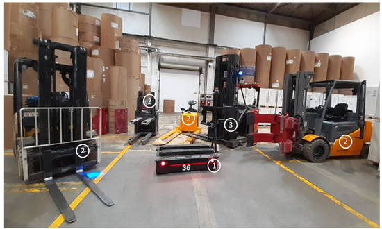
Figure 3. Types of vehicles for internal transportation in printing company: 1–AMR, 2–forklift, 3–forklift for high-bay warehouse.

• Autonomous mobile robots, represented by MiR1000 vehicles, can transfer heavy loads up to 1000 kg. When equipped with a pallet rack, they can pick up and deliver pallets in a completely autonomous way. The newest laser-scanner technology, two 3D cameras in the front, and two sensors in each corner enable the robot to detect obstacles and safely maneuver, even in a highly dynamic environment. Special control algorithms enable to efficiently navigate throughout the warehouse and select the optimal route.
• Human-operated forklift trucks with electric lifting mechanism, represented by Toyota BT LPE200 and YALE MP20XFBW vehicles, are high-speed electric vehicles. They use special forks to transport heavy loads (up to 2000 kg). In contrast to AMRs, they can lift pallets straight from the floor, which means that they do not need any additional equipment. They do not have any safety systems or external anticollision systems. The presence of an operator is controlled by two-hand control system.

4.2. Simulation Data Parameters: Values of Energy Consumption Factor VDI

The energy consumption coefficient VDI is an essential decision attribute in energy efficient optimization of transport processes. Manufacturers of transportation vehicles use the VDI specifications to assess the energy requirements of vehicles in conditions close to those of actual exploitation. However, for autonomous mobile robots, the VDI standard is not defined, which makes it difficult to carry out the energy consumption analysis in production plants equipped with AMRs. To handle this issue, we have carried out cycle tests for AMRs. To be compliant with the VDI 2198 standard, the following settings have been used during the tests: load weight 1000 kg, maximum acceleration, maximum straight-line speed, accordingly, defined routes. The battery of each AMR was initially charged to its maximum capacity, and next several dozens of identical passes were made. We have also defined a typical transportation cycle for AMRs and performed several dozens of passes for this cycle. At the end of each cycle, the battery was reloaded to its maximum capacity, and the electricity consumption was measured each time. On this basis, we have assessed energy consumption for the considered measurement cycles. The obtained results have shown that the energy consumption of AMRs is at least eight times lower compared to the energy consumption of platform forklifts and over 10 times lower than the energy consumption of forklifts. Such a low energy consumption may result from using a brushless drive system and a load-bearing platform that allows to minimize the weight of an AMR. Additionally, the robots are equipped with a system which enables energy to be recovered during braking. The data on the energy consumption of the battery electric vehicles used in the internal transportation system is presented in Table 3.

Table 3. Electric transportation vehicles used for servicing internal transportation requests.

Model	Type	Energy Consumption According to VDI 2198 (kWh/h)	Quantity
MiR 1000	Autonomous	0.03	4
BT LPE200	Human operated	0.46	2
YALE MP20XFBW	Human operated	0.47	3

4.3. Simulation Data Parameters:Transportation Network

The internal transportation network of the considered printing company is represented by a graph with 220 vertices (161 centroid-nodes generating transportation requests and 59 intersection-nodes) and 117 edges (see Figure 4). The centroid-nodes represent origins and/or destinations of the requests for deliveries within the factory’s internal transportation system (these nodes correspond to warehouses and buffers near production machines).

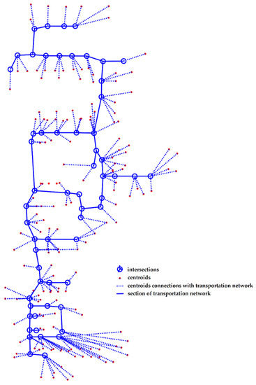
Figure 4. Graph model of internal transportation network in printing company.

The demand for deliveries is represented as material flows of the following types:

• Paper: the raw paper to be delivered to printing machines,
• Intermediate: intermediate products that need further processing,
• Inserts: the intermediate products that should be completed with promotional materials to be inserted manually,
• Ready: ready products (printed materials to be sent to the company’s customers),
• Wastes: the rest of the paper rolls and other printing materials (spare parts for printing machines, painting bins, etc.).

For each type of material flow circulating within the factory, the matrices representing intensities (the number of requests per hour) of the flows were estimated based on the historical data. The number of columns and rows in the matrices is equal to the number of centroids within the network model: the matrix element has zero value if no requests for deliveries between the pair of centroids were observed in the analyzed historical data.

4.4. Other Simulation Assumptions

For each run of the simulation model implementing the processes of servicing the requests for internal transportation deliveries, the following assumptions were considered:

• The duration of the servicing period is 24 h; the electric vehicles service the requests during that period without breaks; all vehicles are involved in the process of servicing the requests for deliveries;
• The technical speed of vehicles is the normally distributed stochastic variable with mean value 5 km/h and standard deviation 1 km/h;
• The duration of loading and unloading operations per each palette in a consignment is a normal random variable with mean value 10 s and standard deviation 2 s;
• The time intervals between consecutive requests in a flow are exponentially distributed random variables with the average value inversely proportional to the intensity of the corresponding flow.

5. Results of Simulations and Discussion

Four scenarios were considered during the simulation experiment:

• BASIC-Manual: only manually operated electric carts are considered; the requests for deliveries are serviced in a standard way, i.e., requests are assigned to electric vehicles based on the current position of available vehicles: the vehicle closest to the sender node is selected;
• OPTIMIZED-Manual: only manually operated electric carts are considered; the assignment is performed as the result of solving the optimization problem of minimizing the total energy consumption of transportation vehicles; the problem is solved for the set of vehicles and not-serviced requests available at the given time;
• BASIC-Autonomous+: both manually operated and autonomous vehicles are considered; the requests for deliveries are serviced in a standard way;
• OPTIMIZED-Autonomous+: both manually operated and autonomous vehicles are considered; the assignment is performed as the result of solving the optimization problem of minimizing the total energy consumption of vehicles.

The procedure of simulating the internal transportation implements the discrete-time approach; the statuses of all elements within the system are checked with the given time span. The time span for both scenarios was set equal to 0.01 h; thus, the assignment procedure for each of the described scenarios is run each 36 s, if the set of available vehicles and the set of requests to serve are not empty at the given moment.

The aim of the experiment is to verify effects of implementing two solutions: an implementing the optimization model for assignment of transportation orders to fleet in internal transport system and a replacement of transportation vehicles with AMRs.

Numerical Results

For each of the described scenarios, the model was run 100 times. For each run of the model, the demand for the internal transport deliveries was generated as described above and the servicing process was simulated for the generated requests. The total servicing time for all electric vehicles and the total consumption of energy by the vehicle’s fleet were estimated for each run of the simulation model.

As the result, we have obtained four sets of samples representing the random variables of the total servicing time and the total energy consumption. The distributions of these stochastic variables are shown in Figure 5 and Figure 6 for scenarios with manually operated vehicles and in Figure 7 and Figure 8 for scenarios when autonomous vehicles are also considered. The hypotheses on the normal distribution were confirmed for each of the presented random variables by using the chi-square Pearson’s test for the level of significance equal to 0.05. The Pearson’s test, in this case, seems to be a sufficiently convincing tool for the confirmation of the normal distribution of the total servicing time and the total energy consumption for each of the simulated strategies, as far as the confirmed normality of the listed random variables is used further to substantiate the size of samples obtained as the result of simulations.

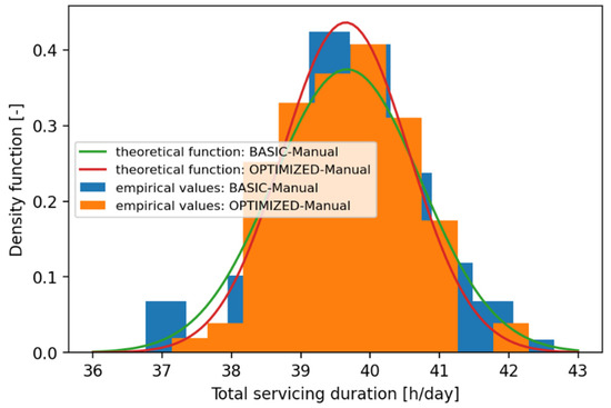
Figure 5. Distribution of total servicing time based on results of simulations (only manually operated vehicles are considered).

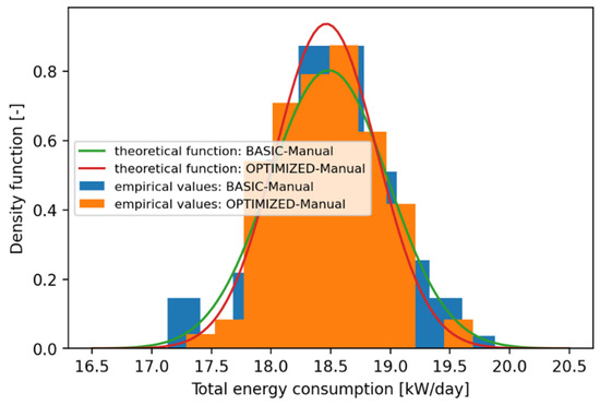
Figure 6. Distribution of energy consumption based on results of simulations (only manually operated vehicles are considered).

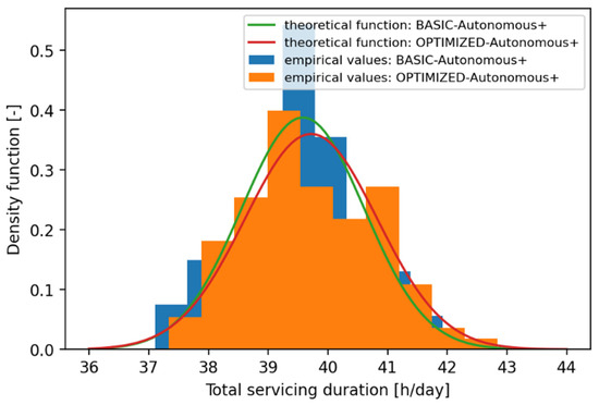
Figure 7. Distribution of total servicing time based on results of simulations (autonomous vehicles are considered).

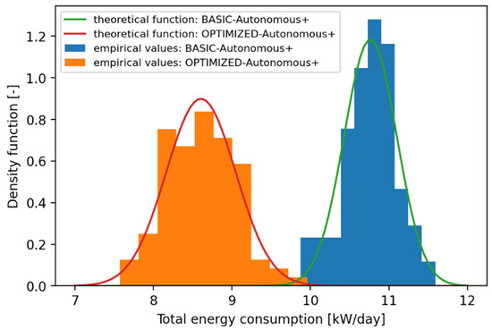
Figure 8. Distribution of energy consumption based on results of simulations (autonomous vehicles are considered).

The most important numeric parameters of the random variables describing the results of the simulation experiment for each of the considered scenarios are presented in Table 4.

Table 4. Numeric results of the simulation experiment.

Parameter	Servicing Strategy
	BASIC-Manual	OPTIMIZED-Manual	BASIC-Autonomous+	OPTIMIZED-Autonomous+
Mean of the total servicing time [h]	39.67	39.65	39.58	39.72
Standard deviation of the total servicing time [h]	1.07	0.92	1.03	1.11
Mean of the total energy consumption [kW/day]	18.48	18.46	10.76	8.60
Standard deviation of the total energy consumption [kW/day]	0.50	0.43	0.34	0.44
Sufficient number of runs	40	39	37	42

The obtained results show that the stochastic variables representing the total duration of servicing operations are very similar for all considered scenarios: these are random values normally distributed in the range between 36 and 44 h per day with an average of about 40 h a day. However, the random variables that describe the total energy consumption differ significantly:

• The average value for the OPTIMIZED-Autonomous+ servicing strategy is 25% lower than the corresponding mean value for the BASIC-Autonomous+ strategy, whereas the range of possible values of the total energy consumption is wider for the optimized variant of servicing the requests for internal transportation (standard deviation is 29% smaller for the conventional variant of the servicing technology);
• The mean value for the OPTIMIZED-Manual servicing strategy is just 0.12% lower than the corresponding average value for the BASIC-Manual strategy;
• Comparing the energy consumption for the OPTIMIZED-Manual and OPTIMIZED-Autonomous+ scenarios, a significant difference could be observed: the use of autonomous vehicles in combination with the proposed optimization procedure allows saving 53.40% of energy for the operation of the electric carts.

The number of observations (runs of the simulation model within the experiment) was estimated to prove that the used samples (100 model runs per scenario) are big enough to ensure statistically significant results. The number of the model runs was calculated for the probability of confidence equal to 0.99 based on the mean values and variations of both resulting indicators—the total servicing duration and the total energy consumption (the bigger value of the number of observations was accepted as the final result). As far as the number of observations is smaller than the number of simulations for all considered scenarios, we conclude that the obtained samples allow obtaining the statistically significant results (for the significance level equal to 0.01).

6. Conclusions

The proposed approach is the first solution presented in the literature to the problem of assignment and scheduling for a mixed fleet of autonomous and manually operated internal transportation vehicles with energy saving objective function. The presented models allow minimizing energy consumption while maintaining the shortest possible routes (and thus total transportation time) and to handle all required transport orders. Moreover, the presented models can reflect many specific constraints, which allows them to be used in various types of production companies, not only in the printing industry. The energy consumption was modeled by the VDI factor described in the VDI 2198 standard, which is based on the typical work cycle of the vehicle, including the operations of lifting and lowering the transported goods. Since such a standard has not been so far defined for the considered MiR1000 vehicles, we performed the measurements that enabled us to determine the VDI value for MiR100 vehicle and what follows to perform the reliable energy consumption tests.

The effectiveness of proposed approach was tested by a simulation model designed for a real-world case study of web printing company. The simulation model was designed with a hybrid approach: it combines the classical components of simulation and the optimization processes. The simulation result presents major conclusions:

• Implementing optimization model in management system of internal transportation produce negligible effects if the system is combined only with human-operated vehicles.
• The changing the human-operated vehicle on autonomous mobile robots could bring the high reduction of energy consumption even if the managing system is not modified.
• Combining two solutions, fleet changing to modern AMRs and implementing the optimization model, could increase the effectiveness of internal transportation system described by energy consumption.
• Using the energy consumption as managing criterion did not negatively influence the quality of services of internal transportation system; the mean service time of transportation vehicles is nearly identical.

In addition to the current fleet control of internal transportation vehicles, the models also allow for the simulation and calculation of the potential savings resulting from the change in the share of autonomous vehicles in relation to the human-operated, less energy-efficient, transportation vehicles. This potentially allow enterprises to better adapt to the rise of energy prices and to the ongoing energy transition. However, autonomous vehicles, especially the most advanced ones like ARM are still too expensive, especially for SMEs, to replace traditional internal transport without clear financial support, e.g., as a part of initiatives to green the financial system.

The solution is currently being implemented as a part of the cyber-physical logistics platform and will be integrated with other systems like dynamic production scheduling and inventory management. In the future, we plan to extend the presented models to optimize charging of AMR vehicles (currently, only the availability or unavailability of the vehicle at a given time is assumed) and include more precise information about the current position of the transportation vehicles (using a real-time localization system).

Appendix A.1. Library for Modeling Transportation System

The library for simulations of processes within the internal transportation system allows describing the system’s main components–the consignors and consignees of loads, the available vehicles fleet, and the processes of transport within the internal transportation network. The structures of the base classes are presented in Figure A1.

The class ITModel represents the model of the process of servicing the requests for deliveries within the production environment. The class contains the following fields mirroring the key subsystems:

• The Graph object represents the transport network (see Figure A1);
• The Demand field is a collection of elements of the Consignment type (see Figure A1); this field is a model of the existing demand for transportation;
• The collection Carts represents the available fleet of vehicles, the collection contains the set of objects of the ElectricCart type;
• The collections Machines and Warehouses of, respectively, the Machinery and the Warehouse elements define the consignees and consignors within the internal transportation system.

The method Run is the key method of the class ITModel that runs the simulation procedure (as the parameter of this method, two alternative variants of the servicing technology are coded by the Boolean variable: true value stands for the requests service based on the approach proposed in this paper, whereas false value represents the conventional, non-optimized, way of servicing). To simulate the demand for internal deliveries, the dedicated method GenerateDemand is used. The procedure DefineIntensities is developed to calculate the intensities for the internal transportation flows based on the movements of vehicles. The method Buffers returns a series representing dynamics of the machine buffers load (the buffers are used for intermediate storage of goods during the production process). The rest of the methods of the ITModel class serve for saving the results of simulations, such as resulting parameters of the vehicles’ operation, the set of simulated requests for transportation, intensities of the generated material flows, the resulting load of sections within the internal transportation network, and the data series for buffers.

Figure A1. UML-diagram of developed base classes for simulations of the internal transportation system.

Figure A1. UML-diagram of developed base classes for simulations of the internal transportation system.

To model the servicing elements of the internal transportation system, the Vehicle abstract class is developed. The procedure Go is the key method of the Vehicle class that checks the status of a servicing element and changes the vehicle parameters (location, status of the serviced request, duration of technological operations) if needed. The ElectricCart class inherits from the Vehicle class and is used for modeling electrically powered servicing machines.

The Machinery class is used to model the production machines, and the Warehouse class to model the warehouses. Both types represent the consignors and consignees within the system of the company’s internal transportation, thus, their key fields within the context of a transportation system are InputPlace and OutputPlace: these parameters are of the Node type (see Figure A2), they are defined as the nodes of the transport network.

Figure A2. UML-diagram of the developed library for modeling the transportation network.

Figure A2. UML-diagram of the developed library for modeling the transportation network.

Appendix A.2. Library for Modeling Transportation Network

To implement the model of the transportation network as a subsystem of the internal transportation system, the corresponding base classes were developed (see Figure A2).

The main class representing the transportation network model is the Graph class; it contains two collections of the graph nodes and vertices and the set of methods that implement basic operations on a graph:

• To define the graph, the AddEdge method is used as the basic procedure. The method allows adding an edge based on the codes of two nodes (optionally, the weight of the edge can be provided as the third element); the nodes with the given codes will be added to the collection Nodes if this collection does not contain such elements; the created edge will be added to the collection Links (if the collection already contains an edge with the given initial and end nodes; and the weight of such the element will be overwritten);
• The graph structure also can be loaded by using the methods LoadNodesFromFile and LoadLinksFromFile: the attributes of the corresponding graph elements should be stored in CSV-files provided as the arguments of the methods; additionally, the LoadFromDB procedure allows the graph structure to be loaded from the database;
• The method ShortestPath returns the shortest path (the object of the Path type) between the source and target nodes (unique codes of the nodes are set as the method’s arguments), the shortest path is calculated based on the Dijkstra’s algorithm; to calculate the shortest distances matrix for all the nodes in the graph, alternatively, the Floyd_Warshall method can be used.

To shape the delivery routes, the Clarke_Wright procedure can be used; for the given sender node, the method returns the collection of the Route objects that represents the set of delivery routes obtained by using the Clarke–Wright heuristic.

The Route class serves for representing the delivery routes as the sequence of the graph nodes (defined by the collection Nodes). The class contains the method Merge that merges the current route with another one (provided as the argument). This procedure is used by the Clarke–Wright heuristic. Additionally, the Route class has the methods for computing the resulting parameters characterizing the given delivery route. The Length function returns the total distance covered by the route, the Beta method estimates the coefficient of the distance utilization by the route, the Gamma method returns the dynamic coefficient of the vehicle’s capacity utilization, and the TransportWork method calculates the total ton-kilometers performed at the route.

The Location class allows representing the location of a point in the two-dimensional space based on the latitude and the longitude coordinates. The object of the Location type may define the location of a graph’s vertex (the Node class contains the corresponding Location field), but also it can be used for defining the track (the shape of the graph’s edge or the shape of the path defined within a graph): the corresponding Track class contains the collection Points of the objects of the Location type.

The dedicated Consignment class should be used to model the requests for deliveries within the transport network; a consignment’s key characteristics are its origin and destination (the Origin and the Destination properties that return the objects of the Node type), and the consignment weight. If the delivery path between the origin and the destination nodes are defined, the shape of the delivery track may be assigned to the corresponding DeliveryTrack field. The process of servicing the request for delivery can be described with the help of the class fields representing time moments for the technological procedures: the request’s appearance in the system (TAppearance), start of loading the consignment on a vehicle (TStartLoad), the start of the transporting the consignment by a vehicle (TStartMove), the start of unloading the consignment from a vehicle (TStartUnload), and finish of servicing (TFinishService). The corresponding statuses of the request servicing process are defined by the inner constants of the Consignment class, and the status may be checked by using the Status field.

To set a flow of requests for deliveries within a transportation network, the Flow class is developed. This class defines the flow between the source and the target vertices (the OutNode and the InNode fields of the Node type) with the given intensity (nonzero value of the field intensity).

References

- Falcone, P.M. Environmental regulation and green investments: The role of green finance. Int. J. Green Econ. 2020, 14, 159. [Google Scholar] [CrossRef]
- Scholz, M.; Kreitlein, S.; Lehmann, C.; Böhner, J.; Franke, J.; Steinhilper, R. Integrating Intralogistics into Resource Efficiency Oriented Learning Factories. Procedia CIRP 2016, 54, 239–244. [Google Scholar] [CrossRef]
- Meißner, M.; Massalski, L. Modeling the electrical power and energy consumption of automated guided vehicles to improve the energy efficiency of production systems. Int. J. Adv. Manuf. Technol. 2020, 110, 481–498. [Google Scholar] [CrossRef]
- Carli, R.; Digiesi, S.; Dotoli, M.; Facchini, F. A Control Strategy for Smart Energy Charging of Warehouse Material Handling Equipment. Procedia Manuf. 2020, 41, 503–510. [Google Scholar] [CrossRef]
- Fazlollahtabar, H.; Saidi-Mehrabad, M. Methodologies to Optimize Automated Guided Vehicle Scheduling and Routing Problems: A Review Study. J. Intell. Robot. Syst. 2015, 77, 525–545. [Google Scholar] [CrossRef]
- Vis, I.F. Survey of research in the design and control of automated guided vehicle systems. Eur. J. Oper. Res. 2006, 170, 677–709. [Google Scholar] [CrossRef]
- Braekers, K.; Ramaekers, K.; Van Nieuwenhuyse, I. The vehicle routing problem: State of the art classification and review. Comput. Ind. Eng. 2016, 99, 300–313. [Google Scholar] [CrossRef]
- Meersmans, P.J.M.; Wagelmans, A.P.M. Effective Algorithms for Integrated Scheduling of Handling Equipment at Automated Container Terminals. ERIM Report Series Reference No. ERS-2001-36-LIS. 2001. Available online: https://papers.ssrn.com/sol3/papers.cfm?abstract_id=370889 (accessed on 6 June 2021).
- Nishi, T.; Hiranaka, Y.; Grossmann, I.E. A bilevel decomposition algorithm for simultaneous production scheduling and conflict-free routing for automated guided vehicles. Comput. Oper. Res. 2011, 38, 876–888. [Google Scholar] [CrossRef]
- Desaulniers, G.; Langevin, A.; Riopel, D.; Villeneuve, B. Dispatching and Conflict-Free Routing of Automated Guided Vehicles: An Exact Approach. Int. J. Flex. Manuf. Syst. 2003, 15, 309–331. [Google Scholar] [CrossRef]
- Rashidi, H.; Tsang, E.P. A complete and an incomplete algorithm for automated guided vehicle scheduling in container terminals. Comput. Math. Appl. 2011, 61, 630–641. [Google Scholar] [CrossRef]
- Zhang, D.; Zhang, C.; Xu, F.; Zuo, D. A hybrid genetic algorithm used in vehicle dispatching for JIT distribution in NC workshop. IFAC-PapersOnLine 2015, 48, 898–903. [Google Scholar] [CrossRef]
- Li, G.; Zeng, B.; Liao, W.; Li, X.; Gao, L. A new AGV scheduling algorithm based on harmony search for material transfer in a real-world manufacturing system. Adv. Mech. Eng. 2018, 10, 1687814018765560. [Google Scholar] [CrossRef]
- Saidi-Mehrabad, M.; Dehnavi-Arani, S.; Evazabadian, F.; Mahmoodian, V. An Ant Colony Algorithm (ACA) for solving the new integrated model of job shop scheduling and conflict-free routing of AGVs. Comput. Ind. Eng. 2015, 86, 2–13. [Google Scholar] [CrossRef]
- Zheng, Y.; Xiao, Y.; Seo, Y. A tabu search algorithm for simultaneous machine/AGV scheduling problem. Int. J. Prod. Res. 2014, 52, 5748–5763. [Google Scholar] [CrossRef]
- Zhang, F.; Li, J. An Improved Particle Swarm Optimization Algorithm for Integrated Scheduling Model in AGV-Served Manufacturing Systems. J. Adv. Manuf. Syst. 2018, 17, 375–390. [Google Scholar] [CrossRef]
- Abdelmaguid, T.; Nassef, A.O.; Kamal, B.A.; Hassan, M.F. A hybrid GA/heuristic approach to the simultaneous scheduling of machines and automated guided vehicles. Int. J. Prod. Res. 2004, 42, 267–281. [Google Scholar] [CrossRef]
- Reddy, B.S.P.; Rao, C.S.P. A hybrid multi-objective GA for simultaneous scheduling of machines and AGVs in FMS. Int. J. Adv. Manuf. Technol. 2006, 31, 602–613. [Google Scholar] [CrossRef]
- Erol, R.; Sahin, C.; Baykasoglu, A.; Kaplanoglu, V. A multi-agent based approach to dynamic scheduling of machines and automated guided vehicles in manufacturing systems. Appl. Soft Comput. 2012, 12, 1720–1732. [Google Scholar] [CrossRef]
- Bilge, U.; Ulusoy, G. A Time Window Approach to Simultaneous Scheduling of Machines and Material Handling System in an FMS. Available online: https://pubsonline.informs.org/doi/abs/10.1287/opre.43.6.1058 (accessed on 6 June 2021).
- Zou, W.Q.; Pan, Q.K.; Meng, T.; Gao, L.; Wang, Y.L. An effective discrete artificial bee colony algorithm for multi-AGVs dis-patching problem in a matrix manufacturing workshop. In Proceedings of the Expert Systems with Applications; Elsevier Ltd.: Amsterdam, The Netherlands, 2020; Volume 161, p. 113675. [Google Scholar]
- Xiao, H.-N.; Lou, P.-H.; Man, Z.-G.; Qian, X.-M. Real-time multi-attribute dispatching method for automatic guided vehicle system. Comput. Integr. Manuf. Syst. 2012, 18, 2224–2230. [Google Scholar]
- Guang, X.P.; Dai, X.; Li, J. Variable neighborhood niche genetic algorithm based AGV flow path design method. China Mech. Eng. 2009, 20, 2581–2586. [Google Scholar]
- Xia, Q.; Ye, X. The application of genetic algorithm in global optimal path searching of AGV. J. Sichuan Univ. 2008, 45, 1129–1136. [Google Scholar]
- Song, L.; Jin, S.; Tang, P. Simulation and optimization of logistics distribution for an engine production line. J. Ind. Eng. Manag. 2016, 9. [Google Scholar] [CrossRef]
- Wang, C.; Guan, Z.; Shao, X.; Ullah, S. Simulation-based optimisation of logistics distribution system for an assembly line with path constraints. Int. J. Prod. Res. 2013, 52, 3538–3551. [Google Scholar] [CrossRef]
- Liang, X.; Sun, Y.; He, X. A hybrid algorithm for routing optimization of AGVs with multi-task assignment. IOP Conf. Series: Earth Environ. Sci. 2018, 189, 062050. [Google Scholar] [CrossRef]
- Corréa, A.I.; Langevin, A.; Rousseau, L.-M. Scheduling and routing of automated guided vehicles: A hybrid approach. Comput. Oper. Res. 2007, 34, 1688–1707. [Google Scholar] [CrossRef]
- Fazlollahtabar, H.; Hassanli, S. Hybrid cost and time path planning for multiple autonomous guided vehicles. Appl. Intell. 2017, 48, 482–498. [Google Scholar] [CrossRef]
- Zhou, B.-H.; Shen, C.-Y. Multi-objective optimization of material delivery for mixed model assembly lines with energy consideration. J. Clean. Prod. 2018, 192, 293–305. [Google Scholar] [CrossRef]
- Angeloudis, P.; Bell, M.G. An uncertainty-aware AGV assignment algorithm for automated container terminals. Transp. Res. Part. E Logist. Transp. Rev. 2010, 46, 354–366. [Google Scholar] [CrossRef]
- Bányai, Á.; Illés, B.; Glistau, E.; Machado, N.I.C.; Tamás, P.; Manzoor, F.; Bányai, T. Smart Cyber-Physical Manufacturing: Extended and Real-Time Optimization of Logistics Resources in Matrix Production. Appl. Sci. 2019, 9, 1287. [Google Scholar] [CrossRef]
- Singh, N.; Sarngadharan, P.V.; Pal, P.K. AGV scheduling for automated material distribution: A case study. J. Intell. Manuf. 2011, 22, 219–228. [Google Scholar] [CrossRef]
- Fazlollahtabar, H.; Es’haghzadeh, A.; Hajmohammadi, H.; Ahangar, A.T. A Monte Carlo simulation to estimate TAGV production time in a stochastic flexible automated manufacturing system: A case study. Int. J. Ind. Syst. Eng. 2012, 12, 243. [Google Scholar] [CrossRef]
Publisher’s Note: MDPI stays neutral with regard to jurisdictional claims in published maps and institutional affiliations. |
© 2021 by the authors. Licensee MDPI, Basel, Switzerland. This article is an open access article distributed under the terms and conditions of the Creative Commons Attribution (CC BY) license (https://creativecommons.org/licenses/by/4.0/).