Non-Fragile H_∞ Nonlinear Observer for State of Charge Estimation of Lithium-Ion Battery Based on a Fractional-Order Model

Abstract

This paper deals with the state of charge (SOC) estimation of lithium-ion battery (LIB) in electric vehicles (EVs). In order to accurately describe the dynamic behavior of the battery, a fractional 2nd-order RC model of the battery pack is established. The factional-order battery state equations are characterized by the continuous frequency distributed model. Then, in order to ensure the effective function of nonlinear function, Lipschitz condition and unilateral Lipschitz condition are proposed to solve the problem of nonlinear output equation in the process of observer design. Next, the linear matrix (LMIS) inequality based on Lyapunov’s stability theory and $H_{\infty }$ method is presented as a description of the design criteria for non-fragile observer. Compared with the existing literature that adopts observers, the proposed method takes the advantages of fractional-order systems in modeling accuracy, the robustness of $H_{\infty }$ method in restricting the unknown variables, and the non-fragile property for tolerating slow drifts on observer gain. Finally, The LiCoO${}_2$ LIB module is utilized to verify the effectiveness of the proposed observer method in different operation conditions. Experimental results show that the maximum estimation accuracy of the proposed non-fragile observer under three different dynamic conditions is less than 2%.

1. Introduction

Due to the huge fossil energy consumption since the industrial revolution, electric vehicles (EVs) have been greatly developed [1]. The key energy source of electric vehicles, lithium-ion batteries (LIBs), is considered to be an important way of energy storage because of its high energy storage per unit volume, stable performance, and the potential for lower production costs [2].The state of charge (SOC) of LIB, defined as the ratio of the remaining capacity to the nominal capacity of the battery is crucial to prevent battery from over-charging or over-discharging, fire, and even explosion. Meanwhile, SOC stands for the most basic parameter in a battery management system (BMS) in EVs. The electrochemistry complexity of the battery’s internal reaction usually causes the high nonlinearities of battery systems. Moreover, in practice, SOC cannot be measured directly by sensors.

In the existing studies, a series of equivalent circuit models (ECMs) is carried out to capture nonlinearities of LIB comprehensively, such as Rint Model [3], Thevenin model [4], 2nd-order RC (resistor-capacitor) model [5], etc. More recently, many researchers have found that nonlinear systems have fractional properties [6]. The fractional-order (FO) battery models, which consist of fractional elements, including Warburg element [7], constant phase element (CPE) [7,8], and fractional capacitor [9,10,11,12], have been introduced to model the nonlinear characteristics of battery. The three electrical components, indeed, can be unified by the same equation. Compared with integer-order (IO) models, fractional-order models can model nonlinearities of battery more accurately to achieve better approximation of the battery system [7,8,11,12]. Among them, the Kalman filter-based approaches [7,9] often suppose that the model and measurement noises are Gaussian, and assume that both the covariance matrix of measurement noise and model error are known. On the other hand, the observer-based approaches [8,11,12] do not demand knowledge on noise distributions which are considered to be more practical, of which the observer in [8] with constant gain was slightly weak in tracking the nonlinear dynamic process. In fact, only for integer-order battery models, the observers with dynamic gain were proposed to adapt the nonlinear dynamics [13,14]. Moreover, in order to improve the role of the observer to suppress the measurement noise and modeling error, the $H_{\infty }$ observers for integer-order battery model were introduced in [15,16]. Finally, note that the fractional-order calculus, an extension of the classical integer-order calculus, is developed in various fields such as control engineering [17,18], signal processing [19,20], and system modeling, including supercapacitors [21] and LIBs [7].

In practical applications, many SOC estimation methods are implemented digitally on microcontrollers [22], and the FOC is also actualized by numerical techniques [7,8,9,10,11,12]. Meanwhile, some perturbations such as external disturbances and slow drifts on the observer gain may cause serious deterioration of the observer performance [20,23,24]. This brings up a fragility problem that has been of great interest in the control theory area [20,24,25,26,27]. As the observer gains are usually obtained from LMIs, which are calculated off-line [8,13,14,15,16], a non-fragile observer that tolerates some perturbations or gain fluctuations [25] and allows for on-line tuning of model parameters to retrench the cost of implementation is essential. The authors of [26] focused on a class of nonlinear fractional-order uncertain systems with bounded perturbation on the observer gain. In [20], the authors dealt with the problem of non-fragile observer design for a class of Lipschitz nonlinear fractional-order systems. In [24,25,27], non-fragile observers based on $H_{\infty }$ performance have been investigated.

For the purpose of capturing nonlinearities of LIB in modeling and considering the advantages of the $H_{\infty }$ observer and its practical applications, a non-fragile $H_{\infty }$ observer method with dynamic gain based on fractional 2nd-order RC model is proposed in this paper. Compared with the existing literature, the main contributions of this paper are as follows:

• Kalman filter-based approaches [7,9] usually assume that the model and measurement noises are Gaussian, which is not the case in actual situations. In order to restrict the effects of the non-Gaussian model and measurement noises [28] for fractional-order battery models, a $H_{\infty }$-based nonlinear observer is proposed. Furthermore, the proposed observer with dynamic gain is also considered to outperform the constant gain observer [8]. The dynamic gain means that the proposed observer can estimate the SOC accurately in various dynamic operation conditions.
• The fragility problem involves a trade-off between implementation accuracy and performance deterioration of the observer implementation. It has caused extensive concern in [20,24,25,26,27,29], but it has not be taken seriously in research areas of SOC estimation. Therefore, to further improve the accuracy of SOC estimation of observer-based methods, we put forward the non-fragile observer. For SOC estimation of fractional-order battery model, the non-fragile observer design criterion for the gain of proposed observer is crucial to solve the fragility problem in practical and real-time applications. Considering the additive perturbation on observer gain with known bound make it implement more properly than the off-line calculation of the observer gain in [8]. Moreover, it is vital to improve the reliability and robustness of all observer-based methods for SOC estimation.

The content of this article is arranged as follows. In Section 2, the fractional-order 2 RC equivalent circuit model of the battery pack is explained. Section 3 consists of experiments and a least-square method mixed with physical behavior based identification method for model parameters. In Section 4, the nonlinear observer design criterion is presented to design the SOC estimator. Experimental validations of the SOC estimation are discussed in Section 5. Conclusions are given in Section 6.

2. Fractional-Order Modeling for LiCoO${}_{\mathbf{2}}$ Lithium-Ion Battery (LIB) Module

2.1. Constant Phase Element (CPE)

The electrochemical impedance spectroscopy (EIS) method is based on the measurement of the electrical voltage response of a LIB by applying a wide frequency range of a.c. signal. CPE is an equivalent electrical circuit component to describe the investigated LIB impedance, that is, an imperfect capacitor [30]. Meanwhile, it was introduced in [31] that the majority of capacitors show fractional properties in practical dynamic conditions. In consequence, the electrical impedance of the CPE could be represented as the following form [9]:

$$\begin{array}{ccc}\hfill Z_{CPE}\left(j\omega \right)& =& \frac{1}{C_{CPE}{\left(j\omega \right)}^{\alpha }},0<\alpha <1\hfill \end{array}$$

(1)

or

$$\begin{array}{ccc}\hfill Z_{CPE}\left(s\right)& =& \frac{1}{C_{CPE}{s}^{\alpha }},s=j\omega ,0<\alpha <1\hfill \end{array}$$

(2)

where $Z_{CPE}\left(j\omega \right)=u_{CPE}\left(j\omega \right)/i_{CPE}\left(j\omega \right)$ is the electrical impedance of the CPE when the a.c. signal $i_{CPE}\left(j\omega \right)$ is applied with frequency $\omega$; $i_{CPE}$ and $u_{CPE}$ denote the current and voltage of the CPE, respectively; $C_{CPE}$ is the capacitance of the CPE, j is the imaginary unit; $\alpha$ is the fractional-order; and s denotes the Laplace variable.

It follows that

$$\begin{array}{c}\hfill \begin{array}{ccc}\hfill i_{CPE}\left(t\right)& =\hfill & \hfill C_{CPE}\frac{d^{\alpha }{u}_{CPE}\left(t\right)}{d{t}^{\alpha }}\end{array}\end{array}$$

(3)

2.2. Fractional 2nd-Order RC Battery Model

The Grünwald–Letnikov (GL) definition for generalized fractional integro-differential system is commonly used.

Definition 1.

The α-th order GL fractional derivative of $x\left(t\right)$ is defined by [9,32]

$$\begin{array}{ccc}\hfill D_t^{\alpha }x\left(t\right)& =& \underset{h\to 0}{lim}{h}^{-\alpha }\sum _{j=0}^{[t/h]}{\omega }_j^{\alpha }x(t-jh),\hfill \end{array}$$

(4)

where$D_t^{\alpha }=\left\{\begin{array}{ccc}& \frac{d^{\alpha }}{d{t}^{\alpha }},\hfill & \hfill \alpha >0\\ & 1,\hfill & \hfill \alpha =0\\ & {\int }_0^{\mathrm{t}}{\left(d\tau \right)}^{\alpha }.\hfill & \hfill \alpha <0\end{array}\right.$is the continuous integro-differential operator, the factor${\omega }_j^{\alpha }={(-1)}^j\left(\genfrac{}{}{0pt}{}{\alpha }{j}\right)$, ${\omega }_0^{\alpha }=1$, $\left(\genfrac{}{}{0pt}{}{\alpha }{j}\right)$is the binomial coefficient, thus${\omega }_j^{\alpha }=(1-\frac{\alpha +1}{j}){\omega }_{j-1}^{\alpha }$, and [t/h] is the integer part of$t/h$.

According to Definition 1, the following GL fractional-order integral form when $\alpha <0$ can be obtained:

$$\begin{array}{c}\hfill D^{\alpha }x\left(t\right)=\begin{array}{c}\hfill {\int }_0^{\mathrm{t}}x\left(\tau \right){\left(d\tau \right)}^{\alpha }=\underset{h\to 0}{lim}{h}^{\alpha }\sum _{j=0}^{[t/h]}{\omega }_j^{-\alpha }x(t-jh).\end{array}\end{array}$$

(5)

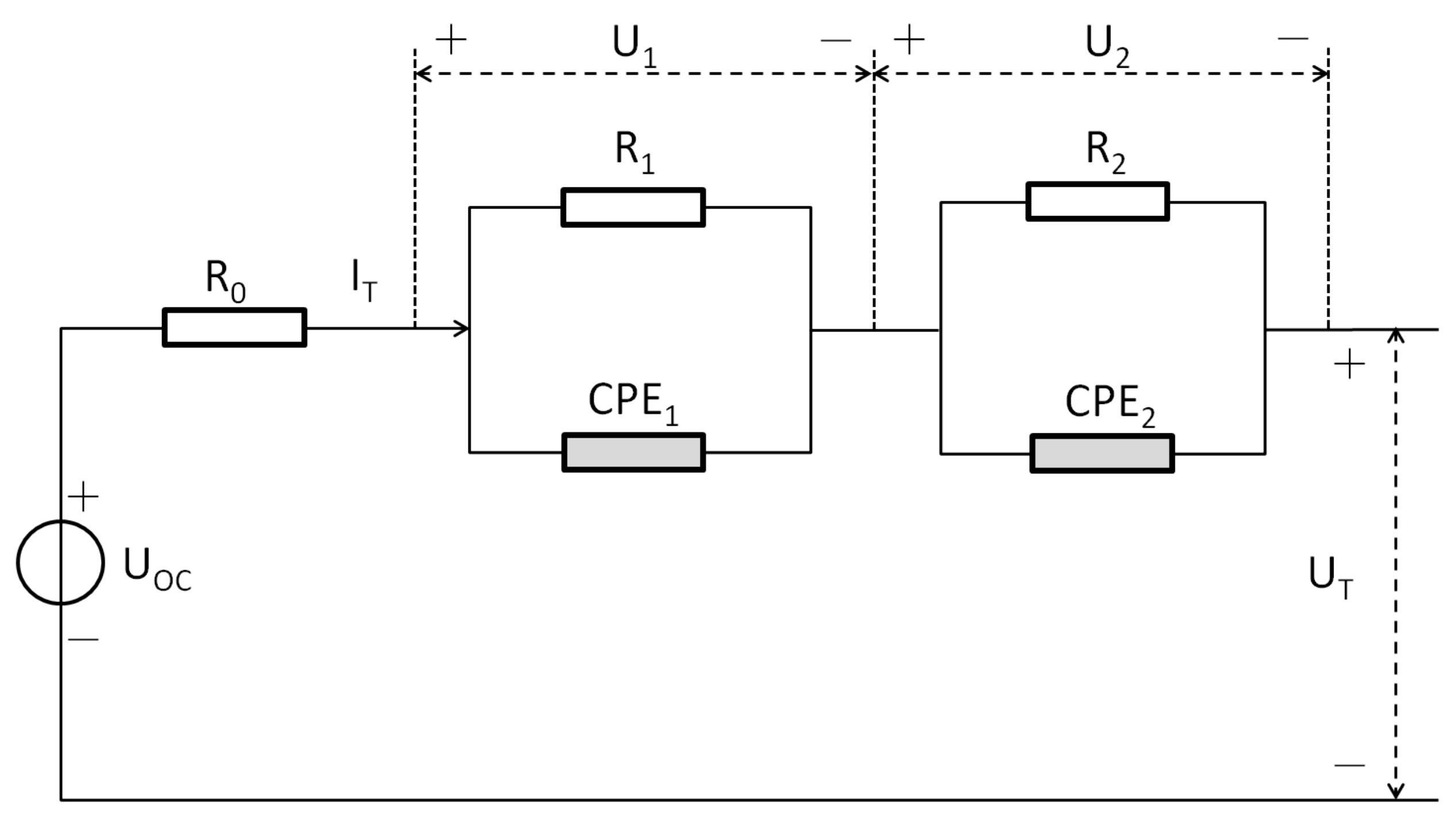
As is mentioned in the introduction, various kinds of ECMs have been widely used in battery modeling, most of which comprise one or more capacitors. Generally, the capacitors of the ECMs are assumed to be integer-order. As is mentioned in [31], the fractional capacitor model can reproduce and predict the capacitor’s behavior much better than any other theory. Considering the fractional properties of capacitor, in this paper, the fractional 2nd-order RC battery model is introduced by adopting two CPEs to replace the two integer-order capacitors in the commonly used integer 2nd-order RC ECM [5,33], which had been studied in [7,8]. Another reason to employ this model is that we find it can perform better in modeling the change of terminal voltage than the integer 2nd-order RC model. As such, the fractional 2nd-order RC ECM is employed here, and its schematic diagram is shown in Figure 1.

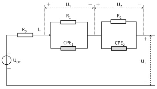
Figure 1. The schematic diagram of the fractional 2nd-order RC model.

In Figure 1, the notation $U_{\mathrm{OC}}$ denotes the OCV related to SOC; $I_T$ is the operating current, which is positive in the discharge process and negative in the charge process; $U_T$ indicates the terminal voltage; and $R_0$ is Ohmic resistance. The notations $R_1$ and $C_1$ are the electrochemical polarization resistance and constant phase element ${\mathrm{CPE}}_1$, respectively. $R_2$ and $C_2$ are the concentration polarization resistance and constant phase element ${\mathrm{CPE}}_2$, respectively. In addition, $U_1$ and $U_2$ denote the voltages of ${\mathrm{CPE}}_1$ and ${\mathrm{CPE}}_2$, respectively.

Next, we will build a battery model based on Kirchhoff Voltage laws with relationship Equation (3).

State Equation:

$$\begin{array}{c}\hfill \left\{\begin{array}{cc}\hfill \frac{d^{{\alpha }_1}{U}_1}{d{t}^{{\alpha }_1}}& =-\frac{1}{R_1{C}_1}{U}_1+\frac{1}{C_1}{I}_T,\hfill \\ \hfill \frac{d^{{\alpha }_2}{U}_2}{d{t}^{{\alpha }_2}}& =-\frac{1}{R_2{C}_2}{U}_2+\frac{1}{C_2}{I}_T,\hfill \\ \hfill \frac{dSOC}{dt}& =-\frac{1}{Q_n}{I}_T.\hfill \end{array}\right.\end{array}$$

(6)

Output equation:

$$\begin{array}{c}\hfill U_T=U_{OC}\left(SOC\right)-R_0{I}_T-U_1-U_2,\end{array}$$

(7)

where $Q_n$ is the nominal capacity of the battery, and $0<{\alpha }_1,{\alpha }_2<1$ are the fractional orders of the ${\mathrm{CPE}}_1$ and ${\mathrm{CPE}}_2$, respectively.

3. Experiments and Identification of Model Parameters

In this section, we want to identify the unknown parameters ${\alpha }_1,{\alpha }_2,R_0,R_1,R_2,C_1,C_2$ and nonlinear function $U_{OC}\left(SOC\right)$ in battery Equations (6) and (7) by experiments. First, let us introduce our test bench.

3.1. Test Bench

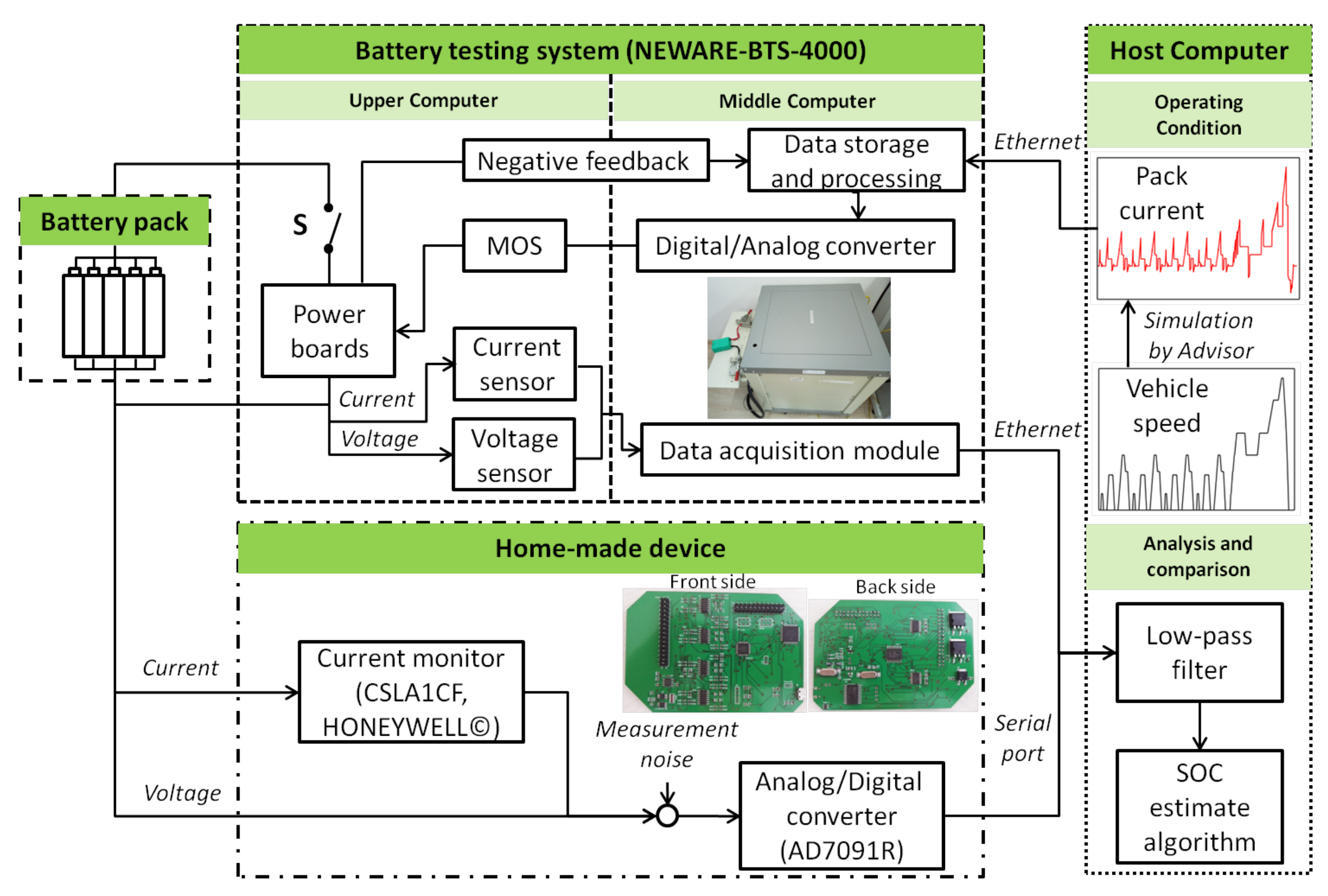
The test bench is illustrated in Figure 2; two sets of devices are used to measure the battery characteristics at the same time and record the battery voltage and current data. Device 1 is NEWARE BTS-4000. Because of its high measurement accuracy and low measurement noise, the measured value of this device is used as a reference value. Meanwhile, using a set of home-made equipment to measure battery voltage and current data, the devices have measurement noise and errors during the data collection process, which can be used to simulate the real measurement environment and verify the effectiveness of the proposed SOC estimation method. Finally, the cell type used in the experiments is NCR18650BE, a LIB with cathode material lithium cobalt oxide and anode material graphite made by Panasonic Corp., Kadoma, Japan. Its nominal voltage is 3.6 V, and the nominal capacity is 3.2 Ah. Moreover, the test object is a battery pack with ten batteries connected in parallel. So the nominal capacity of the battery pack $Q_n$ equals to 32 Ah.

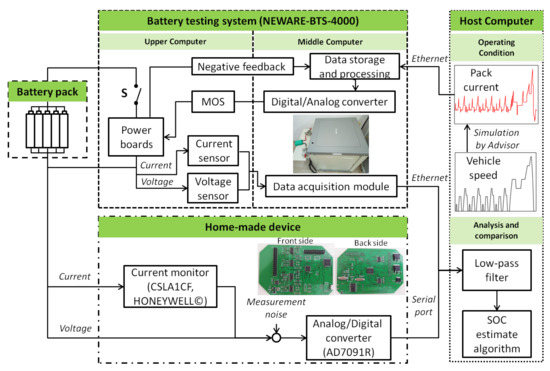
Figure 2. Block diagram of the test bench.

3.2. Parameters and Nonlinear Function Identification

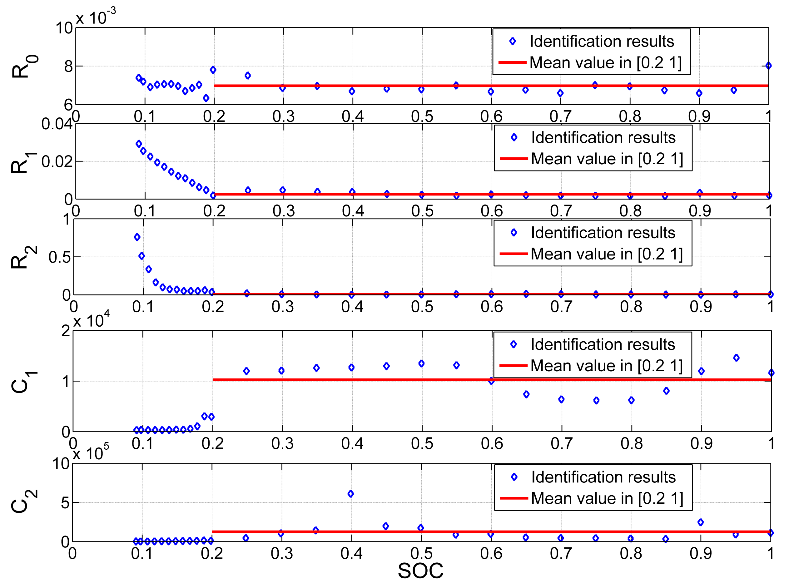
Step 1. Identify the parameters $R_0$, $R_1$, $R_2$, $C_1$, $C_2$, and $U_{OC}\left(SOC\right)$. Here, both the orders ${\alpha }_1$ and ${\alpha }_2$ are assumed to be unity. Using the method employed in [5] with current pulses, these parameters $R_0\left(m\mathsf{\Omega }\right)$, $R_1\left(m\mathsf{\Omega }\right)$, $R_2\left(m\mathsf{\Omega }\right)$, $C_1\left(kF\right)$, and $C_2\left(kF\right)$ are identified as the blue points in Figure 3.

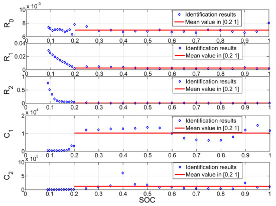
Figure 3. Identification results and mean value in [0.2, 1] of parameters $R_0,R_1,R_2,C_1,C_2$.

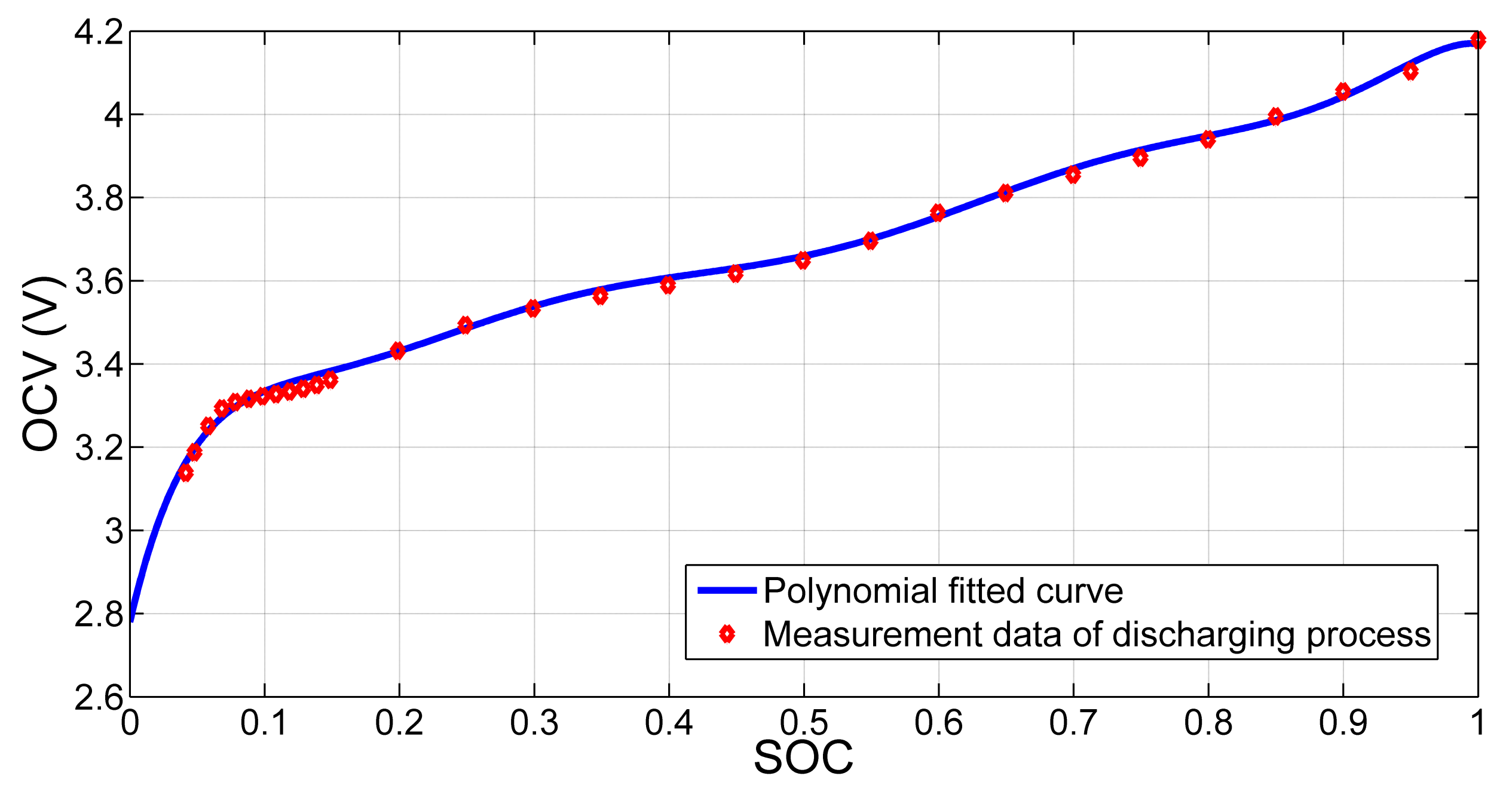
The mean values of the SOC interval $[0.2,1]$ in Figure 3 are set to the constant identified results. The eighth-order polynomial is employed to fit the nonlinear function of OCV and SOC and it is given by

$$\begin{array}{c}\hfill \begin{array}{c}\hfill U_{OC}\left(SOC\right)=p_{1}SO{C}^8+p_{2}SO{C}^7+\dots +p_9,\end{array}\end{array}$$

(8)

where $[p_1,p_2,\dots ,p_9]=[-775.25,3273.15,-5691.59,5264.44,-2795.32,860.49,-148.66,14.13,2.78].$ The measurement data and fitted curve of OCV vs. SOC are shown in Figure 4. As a result, the parameters are shown in Table 1.

Figure 4. Measurement data and fitted curve of OCV vs. SOC.

Table 1. Identification results of the parameters.

${\mathit{\alpha }}_1$	${\mathit{\alpha }}_2$	${\mathit{R}}_0$	${\mathit{R}}_1$	${\mathit{R}}_2$	${\mathit{C}}_1$	${\mathit{C}}_2$
0.91	0.83	6.974	2.604	8.201	10.259	125.688

Step 2. Identify the fractional orders ${\alpha }_1$ and ${\alpha }_2$. Based on the identified parameters in Step 1, the fractional orders ${\alpha }_1$ and ${\alpha }_2$ are further employed to improve modeling accuracy. To this end, the least-square (LS) method is used to minimize the modeling error, that is,

$$\begin{array}{c}\hfill \underset{{\alpha }_1,{\alpha }_2}{min}\sum _{j=1}^N{\parallel U_T^{*}\left(j\right)-U_T\left(j\right)\parallel }^2\end{array}$$

(9)

where N is the number of the samples, $U_T^{*}\left(j\right)$ is the measured terminal voltage, and $U_T\left(j\right)$ is the predictive voltage using the identified model. Notice that for given fractional orders ${\alpha }_1$ and ${\alpha }_2$, the predictive voltage $U_T\left(j\right)$ is given by

$$\begin{array}{c}\hfill \begin{array}{ccc}\hfill U_T& =& U_{OC}\left(SOC\right)-R_0{I}_T\hfill \\ & & -h^{{\alpha }_1}{\displaystyle \sum _{j=0}^k}{\omega }_j^{-{\alpha }_1}\frac{R_{1}I(t-jh)-U_1(t-jh)}{R_1{C}_1}\hfill \\ & & -h^{{\alpha }_2}{\displaystyle \sum _{j=0}^k}{\omega }_j^{-{\alpha }_2}\frac{R_{2}I(t-jh)-U_2(t-jh)}{R_2{C}_2},\hfill \end{array}\end{array}$$

(10)

where h is the sample time. The identification results of parameters ${\alpha }_1$ and ${\alpha }_2$ are also shown in Table 1.

4. Non-Fragile ${\mathit{H}}_{\infty }$ Nonlinear Observer for SOC Estimation Based on Fractional-Order Model

4.1. Battery State-Space Model

The battery Equations (6) and (7) can be rewritten as

$$\begin{array}{c}\hfill \left\{\begin{array}{ccc}\hfill D^{\alpha }\mathit{x}& =& A\mathit{x}+Bu,\mathit{x}\left(0\right)={\mathit{x}}_0,\hfill \\ \hfill y& =& h\left(\mathit{x}\right)+C\mathit{x}-R_{0}u,\hfill \end{array}\right.\end{array}$$

(11)

where $\alpha =[{\alpha }_1,{\alpha }_2,1]$, $\mathit{x}={[U_1,U_2,SOC]}^{\mathrm{T}},y=U_T,u=I_T$, $h\left(\mathit{x}\right)=U_{OC}\left(SOC\right)$, ${\mathit{x}}_0$ is the initial state and

$$\begin{array}{c}\hfill A=\left[\begin{array}{ccc}-\frac{1}{{\tau }_1}& 0& 0\\ 0& -\frac{1}{{\tau }_2}& 0\\ 0& 0& 0\end{array}\right],B=\left[\begin{array}{c}\frac{1}{C_1}\\ \frac{1}{C_2}\\ -\frac{1}{Q_n}\end{array}\right],C^{\mathrm{T}}=\left[\begin{array}{c}-1\\ -1\\ 0\end{array}\right].\end{array}$$

As the battery charging and discharging process involves complicated physical and chemical reactions, the battery Equation (18) are further rewritten as

$$\begin{array}{c}\hfill \left\{\begin{array}{ccc}\hfill D^{\alpha }\mathit{x}& =& A\mathit{x}+Bu+d_x,\mathit{x}\left(0\right)={\mathit{x}}_0,\hfill \\ \hfill y& =& h\left(\mathit{x}\right)+C\mathit{x}-R_{0}u+d_y,\hfill \end{array}\right.\end{array}$$

(12)

where $d_x$ represents the state disturbance caused by the modeling error of current and measurement noise, and $d_y$ represents the output disturbance caused by measurement noise of current and terminal voltage. In the observer-based SOC estimation method, assuming that only $d_x$ and $d_y$ bounded, the range is $\parallel d_x\parallel <\infty$ and $\parallel d_y\parallel <\infty$.

4.2. Discussions for SOC-OCV Function $U_{OC}\left(SOC\right)$

The estimated values of the state $\mathit{x}$ and $SOC$ are $\widehat{\mathit{x}}$ and $\widehat{SOC}$, respectively, and $\tilde{h}\triangleq h\left(\mathit{x}\right)-h\left(\widehat{\mathit{x}}\right)$. The $SOC$ values range from [0,1] and the function of $U_{OC}\left(SOC\right)$ is a monotonically increasing. Then, we have

$$\begin{array}{c}\hfill {\beta }_{min}\le {\dot{U}}_{OC}\left(SOC\right)\le {\beta }_{max},\end{array}$$

(13)

with ${\beta }_{min},{\beta }_{max}>0$. In addition, the battery used in the experiment during the test, according to the SOC-OCV curve Equation (8), is satisfied by the the above Equation (13) with

$$\begin{array}{c}\hfill {\beta }_{min}=0.4551,{\beta }_{max}=4.4708.\end{array}$$

(14)

In order to design a nonlinear observer for the above system Equation (12), we first need to discuss the properties of the nonlinear function $h\left(\mathit{x}\right)$.

There exists matrix Q, W, for any $\mathit{x},\widehat{\mathit{x}}$ with $SOC,\widehat{SOC}\in [0,1]$, such that the nonlinear functions $h\left(\mathit{x}\right)$ satisfies the following one-sided Lipschitz condition Equation (15) and Lipschitz condition Equation (16):

$$\begin{array}{c}\hfill -{\tilde{\mathit{x}}}^{\mathrm{T}}{\left[\frac{\partial h}{\partial \mathit{x}}\right]}_{\mathit{x}=\widehat{\mathit{x}}}^{\mathrm{T}}\tilde{h}\le -{\tilde{\mathit{x}}}^{\mathrm{T}}Q\tilde{\mathit{x}},\end{array}$$

(15)

$$\begin{array}{c}\hfill {\tilde{h}}^{\mathrm{T}}\tilde{h}\le {\tilde{\mathit{x}}}^{\mathrm{T}}{W}^2\tilde{\mathit{x}},\end{array}$$

(16)

where $Q=\left[\begin{array}{ccc}0& 0& 0\\ 0& 0& 0\\ 0& 0& {\beta }_{min}^2\end{array}\right],W=\left[\begin{array}{ccc}0& 0& 0\\ 0& 0& 0\\ 0& 0& {\beta }_{max}^2\end{array}\right].$

Proof. 

Please see the authors’ previous work [5]. □

4.3. Non-Fragile Observer Designed for SOC Estimation

The following two lemmas are crucial for designing the observer based on fractional-order model and establish non-fragile observer design criterion, respectively.

Lemma 1.

The factional-order system [17,18,19]

$$\begin{array}{c}\hfill D_t^{\alpha }x\left(t\right)=f\left(x\left(t\right)\right),\end{array}$$

(17)

can be characterized by the continuous frequency distributed model

$$\begin{array}{c}\hfill \left\{\begin{array}{ccc}\hfill \frac{\partial Z_x(\omega ,t)}{\partial t}& =& -\omega Z_x(\omega ,t)+f\left(x\left(t\right)\right),\hfill \\ \hfill x\left(t\right)& =& {\int }_0^{\infty }\mu \left(\omega \right)Z_x(\omega ,t)d\omega ,\hfill \end{array}\right.\end{array}$$

(18)

where ω is the elementary frequency,$z_x(\omega ,t)$is the infinite dimension distributed state variable, and$\mu \left(\omega \right)=\frac{sin\left(\alpha \pi \right)}{\pi }{\omega }^{-\alpha }$.

Lemma 2.

Ref. [20] Let$X\in {\mathit{R}}^n,Y\in {\mathit{R}}^n,$and$\epsilon >0$. Then we have$X^{\mathrm{T}}Y+Y^{\mathrm{T}}X\le \epsilon Y^{\mathrm{T}}Y+\frac{1}{\epsilon }{X}^{\mathrm{T}}X.$

Considering the application of the above mentioned observer-based methods [5,8,11,12,13,14], the non-fragile observer design criterion is introduced here. These observers would be implemented digitally on microcontrollers as many other SOC estimation methods [22]. Meanwhile, as is mentioned in [8], the real application of FOC should be actualized on microcontrollers by numerical techniques. However, the electrical signal loss or interference on the D/A converter (DAC) and Hall sensor is unavoidable in the signals’ conversion and transmission process. Besides, there exist rounding error when the microcontroller unit (MCU) processes floating point numbers, thermal noise of electric conductor, stray electromagnetic field interference, etc. All these bring perturbations to the observer gain lead to a fragility problem, and the fragility problem indeed requires a trade-off of observer implementation accuracy and performance deterioration [23]. Thus, if the fragility problem is not considered, the estimation accuracy of observer-based methods will not be ideal enough as it is designed by $H_{\infty }$ performance. The non-fragile observer provides a optimization algorithm to improve practicability of SOC estimation.

Therefore, we further develop the nonlinear observer based on integer-order model in [5,13,14] to a non-fragile observer based on fractional-order model that tolerates some perturbations as follows:

$$\begin{array}{c}\hfill \left\{\begin{array}{c}{D}^{\alpha }\widehat{\mathit{x}}=A\widehat{\mathit{x}}+Bu+(L+\Delta L)\mathrm{H}\left(\widehat{\mathit{x}}\right)(y-\widehat{y}),\widehat{\mathit{x}}\left(0\right)={\widehat{\mathit{x}}}_0,\hfill \\ \widehat{y}=h\left(\widehat{\mathit{x}}\right)+C\widehat{\mathit{x}}-R_{0}u,\hfill \end{array}\right.\end{array}$$

(19)

where $\widehat{y}$ is the estimate of the real terminal voltage y, L is a matrix that will be designed later, but the vector $(L+\Delta L){\left[\frac{\partial h}{\partial \mathit{x}}\right]}_{\mathit{x}=\widehat{\mathit{x}}}^{\mathrm{T}}$ is the actual observer gain that is dynamic. Let ${\left[\frac{\partial h}{\partial \mathit{x}}\right]}_{\mathit{x}=\widehat{\mathit{x}}}^{\mathrm{T}}\triangleq \mathrm{H}\left(\widehat{\mathit{x}}\right)$ for simplification. $\Delta L\mathrm{H}\left(\widehat{\mathit{x}}\right)$ is additive perturbation on the error gain with the bound satisfying $\parallel \Delta L\parallel \le \delta$ and $\delta$ is a positive constant. Note that the upper bound $\delta$ will be calculated later. It follows that the error dynamics is given by

$$\begin{array}{c}\hfill \begin{array}{cc}{D}^{\alpha }\tilde{\mathit{x}}=\hfill & (A-(L+\Delta L)\mathrm{H}\left(\widehat{\mathit{x}}\right)C)\tilde{\mathit{x}}-(L+\Delta L)\mathrm{H}\left(\widehat{\mathit{x}}\right)\tilde{h}\hfill \\ & +(E-(L+\Delta L)\mathrm{H}\left(\widehat{\mathit{x}}\right)F)\mathit{d}\hfill \end{array}\end{array}$$

(20)

where $\mathit{d}=\left[\begin{array}{c}{d}_x\\ d_y\end{array}\right]$ is the synthetic disturbance, $E=[I_0,0],F=[0,1]$, and $I_0$ denotes the appropriate dimensional identity matrix.

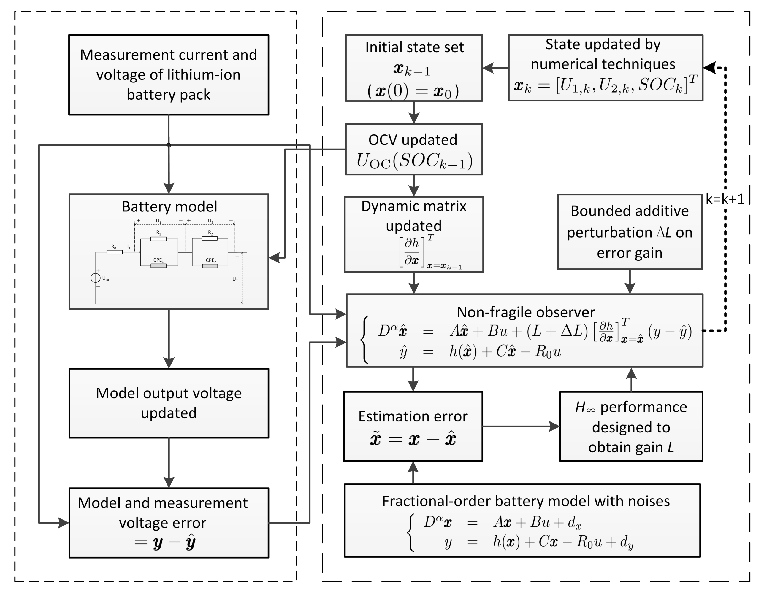
The main contribution of this paper, the non-fragile $H_{\infty }$ design criteria with $H_{\infty }$ performance, is then established as shown in the Figure 5.

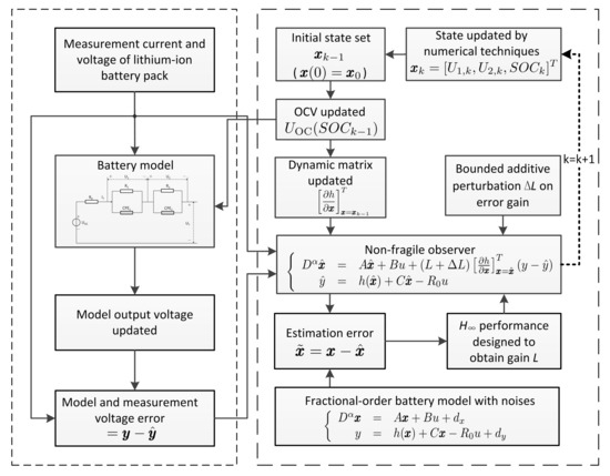
Figure 5. The implement flowchart of non-fragile $H_{\infty }$ observer.

Theorem 1.

Regarding to the non-fragile observer Equation (19), it has a stable observation under system disturbance Equation (12), for given positive scalars$ϵ<2{\beta }_{min}^2$, and γ, if there exist positive real number${\epsilon }_1$,${\epsilon }_2$,${\epsilon }_3$, matrix$P=P^{\mathrm{T}}>0$and vector S, while the observer gain L is the solution of the following LMIs:

$$\begin{array}{c}\hfill \left\{\begin{array}{c}\Xi <0\\ R_{2}S<{\beta }_{max}\\ R_{2}S>{\beta }_{min}\end{array}\right.\end{array}$$

(21)

where$\begin{array}{c}\begin{array}{c}\Xi =\left[\begin{array}{ccccc}{\Xi }_{11}& PE-R_{1}SF& P& P& P\\ & {\Xi }_{22}& 0& 0& 0\\ & & -\frac{1}{{\epsilon }_1}{I}_0& 0& 0\\ & *& & -\frac{1}{{\epsilon }_2}{I}_0& 0\\ & & & & -\frac{1}{{\epsilon }_3}{I}_0\end{array}\right]\hfill \end{array}\end{array}$and${\Xi }_{11}=PA+A^{\mathrm{T}}P-R_{1}SC$$-C^{\mathrm{T}}{S}^{\mathrm{T}}{R}_1^{\mathrm{T}}+ϵI_0-2Q+{\delta }_1{C}^{\mathrm{T}}C+{\delta }_{2}W$,${\Xi }_{22}={\delta }_3{F}^{\mathrm{T}}F-{\gamma }^2{I}_0$,${\delta }_1=\frac{{\delta }^2}{{\epsilon }_1}$,${\delta }_2=\frac{{\delta }^2}{{\epsilon }_2}$,${\delta }_3=\frac{{\delta }^2}{{\epsilon }_3}$, then the battery Equation (12) and the non-fragile nonlinear observer Equation (19)$L=P^{-1}$satisfy the$H_{\infty }$performance with the given attenuation$\gamma >0$, that is

$$\begin{array}{c}\hfill {\int }_{t=0}^{\Gamma }\parallel \tilde{\mathit{x}}{\parallel }^2\mathrm{d}t<{\lambda }_{max}\left(P\right)\parallel \tilde{\mathit{x}}{\left(0\right)\parallel }^2+\frac{{\gamma }^2}{ϵ}{\int }_0^{\Gamma }{\parallel \mathit{d}\left(t\right)\parallel }^2\mathrm{d}t\end{array}$$

(22)

for any$\Gamma >0$.

Proof. 

From Lemma 1, the observer error dynamic system Equation (20) can characterized by

$$\begin{array}{c}\hfill \left\{\begin{array}{ccc}\hfill \frac{\partial {\mathit{Z}}_{\tilde{\mathit{x}}}(\omega ,t)}{\partial t}& =& -\omega {\mathit{Z}}_{\tilde{\mathit{x}}}(\omega ,t)+D^{\alpha }\tilde{\mathit{x}},\hfill \\ \hfill \tilde{\mathit{x}}& =& {\int }_0^{\infty }\mu \left(\omega \right){\mathit{Z}}_{\tilde{\mathit{x}}}(\omega ,t)d\omega ,\hfill \end{array}\right.\end{array}$$

(23)

where $\mu \left(\omega \right)=\mathrm{diag}\{{\mu }_1\left(\omega \right),{\mu }_2\left(\omega \right),{\mu }_3\left(\omega \right)\}=\mathrm{diag}\{\frac{sin\left({\alpha }_1\pi \right)}{\pi }{\omega }^{-{\alpha }_1},\frac{sin\left({\alpha }_2\pi \right)}{\pi }{\omega }^{-{\alpha }_2},\frac{sin\pi }{\pi }{\omega }^{-1}\}$. Note that for $0<{\alpha }_i<1,i=1,2$, $\omega >0$, ${\mu }_i\left(\omega \right)=\frac{sin\left({\alpha }_i\pi \right)}{\pi }{\omega }^{-{\alpha }_i}$ and $\frac{sin\pi }{\pi }{\omega }^{-1}$ are always positive. Therefore, let the candidate of the Lyapunov function be

$$\begin{array}{c}\hfill V\left(\mathit{x}\right)={\int }_0^{\infty }\mu \left(\omega \right){\mathit{Z}}_{\tilde{\mathit{x}}}^{\mathrm{T}}(\omega ,t)P{\mathit{Z}}_{\tilde{\mathit{x}}}(\omega ,t)d\omega ,\end{array}$$

(24)

and the observer gain $L=P^{-1}$.

Taking the derivative of $V\left(\mathit{x}\right)$ along the error System (20) causes

$$\begin{array}{c}\hfill \begin{array}{c}\hfill \dot{V}\left(\mathit{x}\right)=2{\int }_0^{\infty }\mu \left(\omega \right){\mathit{Z}}_{\tilde{\mathit{x}}}^{\mathrm{T}}P\left[-\omega {\mathit{Z}}_{\tilde{\mathit{x}}}(\omega ,t)+D^{\alpha }\tilde{\mathit{x}}\right]d\omega .\end{array}\end{array}$$

(25)

$$\begin{array}{c}\hfill \begin{array}{cc}\hfill \dot{V}\left(\mathit{x}\right)=& 2{\int }_0^{\infty }\mu \left(\omega \right){\mathit{Z}}_{\tilde{\mathit{x}}}^{\mathrm{T}}P\left[-\omega {\mathit{Z}}_{\tilde{\mathit{x}}}(\omega ,t)+D^{\alpha }\tilde{\mathit{x}}\right]d\omega ,\hfill \\ \hfill \le & 2{\tilde{\mathit{x}}}^{\mathrm{T}}P{D}^{\alpha }\tilde{\mathit{x}}d\omega \hfill \\ \hfill \le & 2{\tilde{\mathit{x}}}^{\mathrm{T}}[(PA-R_{1}SC-Q)\tilde{\mathit{x}}+(PE-R_{1}SF)\mathit{d}]-2{\tilde{\mathit{x}}}^{\mathrm{T}}P\Delta L\mathrm{H}\left(\widehat{\mathit{x}}\right)C\tilde{\mathit{x}}\hfill \\ \hfill -& 2{\tilde{\mathit{x}}}^{\mathrm{T}}P\Delta L\mathrm{H}\left(\widehat{\mathit{x}}\right)\tilde{h}-2{\tilde{\mathit{x}}}^{\mathrm{T}}P\Delta L\mathrm{H}\left(\widehat{\mathit{x}}\right)F\mathit{d},\hfill \end{array}\end{array}$$

(26)

$$\begin{array}{c}\hfill \begin{array}{cc}\hfill \dot{V}\left(\mathit{x}\right)\le & 2{\tilde{\mathit{x}}}^{\mathrm{T}}[(PA-R_{1}SC-Q)\tilde{\mathit{x}}+(PE-R_{1}SF)\mathit{d}]+{\epsilon }_1{\tilde{\mathit{x}}}^{\mathrm{T}}P{P}^{\mathrm{T}}\tilde{\mathit{x}}\hfill \\ \hfill +& {\epsilon }_2{\tilde{\mathit{x}}}^{\mathrm{T}}P{P}^{\mathrm{T}}\tilde{\mathit{x}}+{\epsilon }_3{\tilde{\mathit{x}}}^{\mathrm{T}}P{P}^{\mathrm{T}}\tilde{\mathit{x}}\hfill \\ & +\frac{1}{{\epsilon }_1}{\tilde{\mathit{x}}}^{\mathrm{T}}{C}^{\mathrm{T}}{\mathrm{H}}^{\mathrm{T}}\left(\widehat{\mathit{x}}\right)\Delta L^{\mathrm{T}}\Delta L\mathrm{H}\left(\widehat{\mathit{x}}\right)C\tilde{\mathit{x}}+\frac{1}{{\epsilon }_2}{\tilde{h}}^{\mathrm{T}}{\mathrm{H}}^{\mathrm{T}}\left(\widehat{\mathit{x}}\right)\Delta L^{\mathrm{T}}\Delta L\mathrm{H}\left(\widehat{\mathit{x}}\right)\tilde{h}\hfill \\ \hfill +& \frac{1}{{\epsilon }_3}{\mathit{d}}^{\mathrm{T}}{F}^{\mathrm{T}}{\mathrm{H}}^{\mathrm{T}}\left(\widehat{\mathit{x}}\right)\Delta L^{\mathrm{T}}\Delta L\mathrm{H}\left(\widehat{\mathit{x}}\right)F\mathit{d},\hfill \\ \hfill \le & 2{\tilde{\mathit{x}}}^{\mathrm{T}}[(PA-R_{1}SC-Q+\frac{1}{2}({\epsilon }_1+{\epsilon }_2+{\epsilon }_3)P{P}^{\mathrm{T}}+\frac{{\delta }^2}{2{\epsilon }_1}{C}^{\mathrm{T}}C+\frac{{\delta }^2}{2{\epsilon }_2}W)\tilde{\mathit{x}}\hfill \\ \hfill +& (PE-R_{1}SF)\mathit{d}]+{\mathit{d}}^{\mathrm{T}}\frac{{\delta }^2}{{\epsilon }_3}{F}^{\mathrm{T}}F\mathit{d}.\hfill \end{array}\end{array}$$

(27)

By applying $L=P^{-1}$ and the oneside Lipschitz condition Equation (15), and substituting the term $\tilde{\mathit{x}}\left(t\right)$ in Equation (23), the above Equation (25) can be rewritten as Equation (26) at the top of the next page.

Whereas $\parallel \Delta L\mathrm{H}\left(\widehat{\mathit{x}}\right)\parallel \le \delta$, applying Lemma 2 and the Lipschitz condition Equation (16) to Equation (26) concludes Equation (27) at the top of the next page.

To establish then $H_{\infty }$ performance, we have

$$\begin{array}{c}\hfill \dot{V}\left(\mathit{x}\right)+ϵ{\tilde{\mathit{x}}}^{\mathrm{T}}\tilde{\mathit{x}}-{\gamma }^2{\mathit{d}}^{\mathrm{T}}\mathit{d}<0,\end{array}$$

(28)

where $ϵ<2{\beta }_{min}^2$ is used to guarantee that the matrix ${\Xi }_{11}$ could be negative definite. Applying the Schur complement lemma to Equation (28), it is clear to get:

$$\begin{array}{c}\hfill {\left[\begin{array}{c}\tilde{\mathit{x}}\\ \mathit{d}\end{array}\right]}^{\mathrm{T}}\Xi \left[\begin{array}{c}\tilde{\mathit{x}}\\ \mathit{d}\end{array}\right]<0,\end{array}$$

(29)

where $\Xi$ is defined by criterion Equation (21). Therefore, we see that

$$\begin{array}{c}\hfill \Xi <0,R_{2}S<{\beta }_{max},R_{2}S>{\beta }_{min}\end{array}$$

(30)

which yield to Equation (21). Note that ${\int }_0^{\Gamma }\dot{V}\left(\tilde{\mathit{x}}\right)\mathrm{d}t=V(\Gamma )-V\left(0\right)\ge -V\left(0\right)\ge -{\lambda }_{max}\left(P\right)$

$\parallel \tilde{\mathit{x}}{\left(0\right)\parallel }^2$. Therefore, we have ${\int }_0^{\Gamma }{\tilde{\mathit{x}}}^{\mathrm{T}}\tilde{\mathit{x}}\mathrm{d}t\le \frac{{\lambda }_{max}\left(P\right)}{ϵ}{\parallel \tilde{\mathit{x}}\left(0\right)\parallel }^2+\frac{{\gamma }^2}{ϵ}{\int }_0^{\Gamma }{\mathit{d}}^{\mathrm{T}}\mathit{d}\mathrm{d}t$ for any $\Gamma >0$. Therefore, the criterion Equations (21) and (22) could be directly proved. This ends the proof. □

5. Experimental Validations of the SOC Estimation

5.1. Calculate the Gain L and Bound $\delta$

In the subsection, the LMIs (21) are utilized to calculate the gain L. However, the upper bound $\delta$ of uncertainty $\Delta L$ is unknown in practice. As such, the gain L is obtained by solving the following optimization problem (21):

$$\begin{array}{c}\hfill \underset{L}{max}\delta \mathrm{s}.\mathrm{t}.\mathrm{LMIs}.\end{array}$$

(31)

Here, the purpose is to obtain the greatest robustness for the unknown uncertainty $\Delta L$.

Using the MATLAB LMI Toolbox [34] to solve the convex optimization problem (31), the feasible solutions of design critiron Equation (21) with $ϵ=0.1$ in Theorem 1 can be obtained and some of them are list by $\gamma =5.36$, $\delta =1.864\times {10}^{-2}$ and ${\epsilon }_1=1.35\times {10}^{-7},$${\epsilon }_2=7.46\times {10}^{-7},$${\epsilon }_3=1.03\times {10}^{-9},$

$$\begin{array}{c}\hfill L=\left[\begin{array}{ccc}1.21\times {10}^{-5}& 8.72\times {10}^{-8}& 4.36\times {10}^{-7}\\ 8.72\times {10}^{-8}& 2.32\times {10}^{-4}& 3.27\times {10}^{-4}\\ 4.36\times {10}^{-7}& 3.27\times {10}^{-4}& 0.0055\end{array}\right].\end{array}$$

(32)

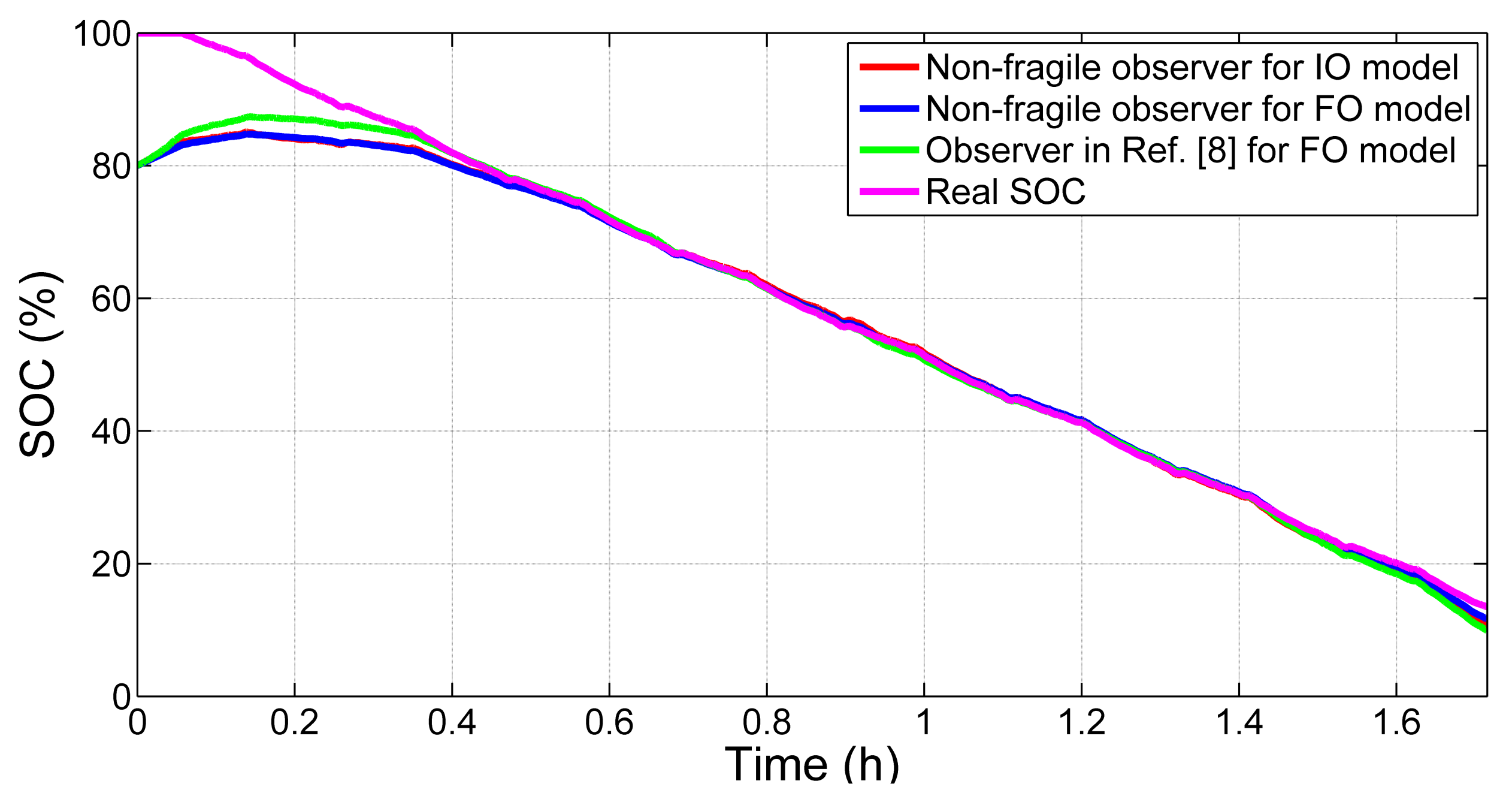
In addition, the observer in [8] is used to highlight the advantages of the nonlinear observer proposed in this paper. Note that in the following figures, the lines named as Real SOC are directly obtained by the standard measurement data based on the ampere-hour counting, but the other lines are calculated by the home-made measurement data.

5.2. Numerical Implementation and Issue for Fractional-Order Observer

There are several numerical methods for fractional-order systems implementations [6,8]. The most commonly used among them is the aforementioned approximate GL definition, where the step size of h is assumed to be very small. By GL definition, the numerical implementation for proposed fractional-order observer Equation (19) is obtained as

$$\begin{array}{c}\hfill \begin{array}{cc}\hfill \widehat{\mathit{x}}(k+1)=& (A{h}^{\alpha }+\mathrm{diag}\left(\alpha \right))\widehat{\mathit{x}}\left(k\right)\hfill \\ & -\sum _{i=2}^{k+1}{(-1)}^i\left(\genfrac{}{}{0pt}{}{\alpha }{j}\right)\widehat{\mathit{x}}(k+1-i)\hfill \\ & +B{h}^{\alpha }u\left(k\right)+h^{\alpha }L{\left[\frac{\partial h}{\partial \mathit{x}}\right]}_{\mathit{x}=\widehat{\mathit{x}}\left(k\right)}^{\mathrm{T}}(y\left(k\right)-\widehat{y}\left(k\right)),\hfill \end{array}\end{array}$$

(33)

for $k\ge 1$, and $\widehat{\mathit{x}}\left(1\right)=(A{h}^{\alpha }+\mathrm{diag}\left(\alpha \right))\widehat{\mathit{x}}\left(0\right)+B{h}^{\alpha }u\left(0\right)+h^{\alpha }L{\left[\frac{\partial h}{\partial \mathit{x}}\right]}_{\mathit{x}=\widehat{\mathit{x}}\left(0\right)}^{\mathrm{T}}(y\left(0\right)-\widehat{y}\left(0\right)),\widehat{\mathit{x}}\left(0\right)={\widehat{\mathit{x}}}_0$,

$$\begin{array}{ccc}\hfill y\left(k\right)& =& h\left(\widehat{\mathit{x}}\left(k\right)\right)+C\widehat{\mathit{x}}\left(k\right)-R_{0}u\left(k\right),\hfill \end{array}$$

(34)

where $h^{\alpha }=\mathrm{diag}\left\{h^{{\alpha }_1}{h}^{{\alpha }_2}h\right\}$, $\left(\genfrac{}{}{0pt}{}{\alpha }{j}\right)=\mathrm{diag}\left\{\left(\genfrac{}{}{0pt}{}{{\alpha }_1}{j}\right)\left(\genfrac{}{}{0pt}{}{{\alpha }_2}{j}\right)\left(\genfrac{}{}{0pt}{}{1}{j}\right)\right\}$. Note that L is substituted by $L+\Delta L$ for proposed non-fragile observer (19). Note that the short memory principle [6,35] is adopted to overcome the increasing amount of calculation from the second term on the right side of Equation (33).

5.3. Experimental Results

We adopt three operation condition: the urban dynamometer driving schedule (UDDS), the new European driving cycle (NEDC), and the highway fuel economy test (HWFET) cycle to evaluate the SOC estimation accuracy of the proposed observer methods. In order to show accurately the SOC estimation results of proposed non-fragile observer for IO model (IONFO) and FO model (FONFO) and the observer for FO model in [8], the mean SOC estimation errors of the above observers are demonstrated in Table 2.

Table 2. Mean/maximum SOC estimation errors of observers after convergence.

Operation Condition	UDDS	NEDC	HWFET
IONFO	0.85%/2.62%	0.71%/1.64%	0.51%/2.72%
FONFO	0.73%/1.64%	0.53%/1.24%%	0.41%/1.83%
Observer in Ref. [8]	0.83%/3.44%	0.94%/2.23%	0.55%/3.58%

5.3.1. UDDS

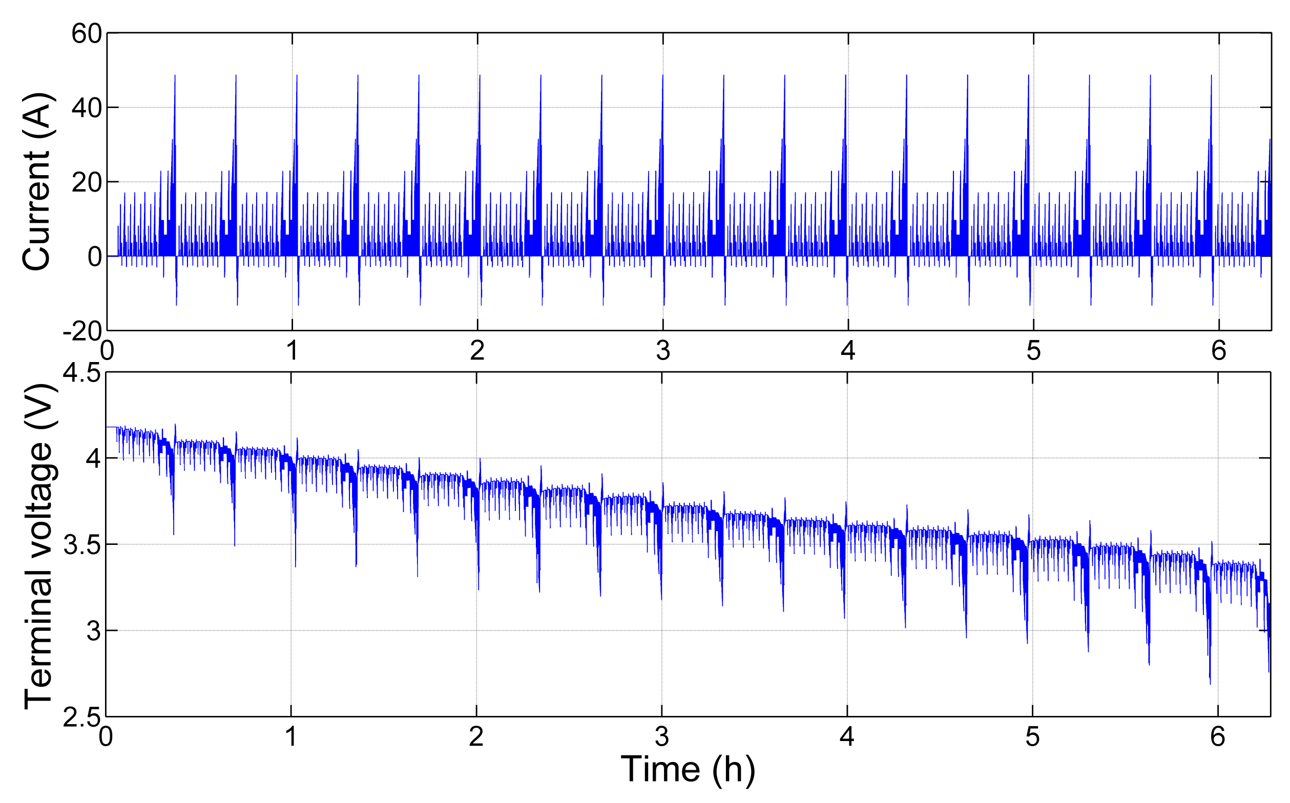
The current and terminal voltage profiles are shown in Figure 6. The SOC estimation profiles and the SOC estimation error profiles are shown in Figure 7 and Figure 8, respectively.

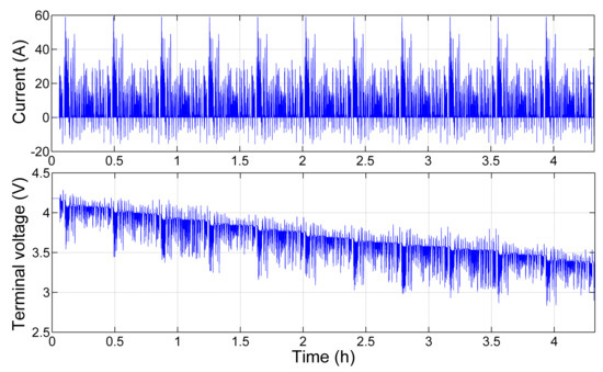
Figure 6. Current and terminal voltage profiles of UDDS.

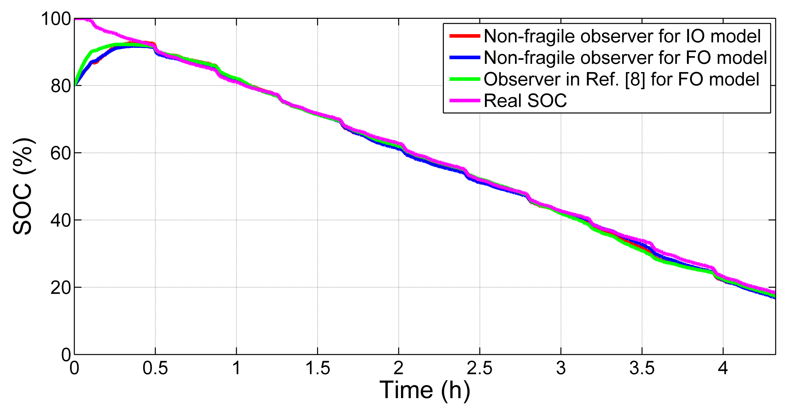
Figure 7. SOC estimation profiles for UDDS.

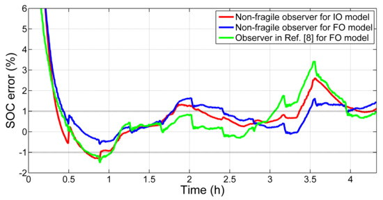
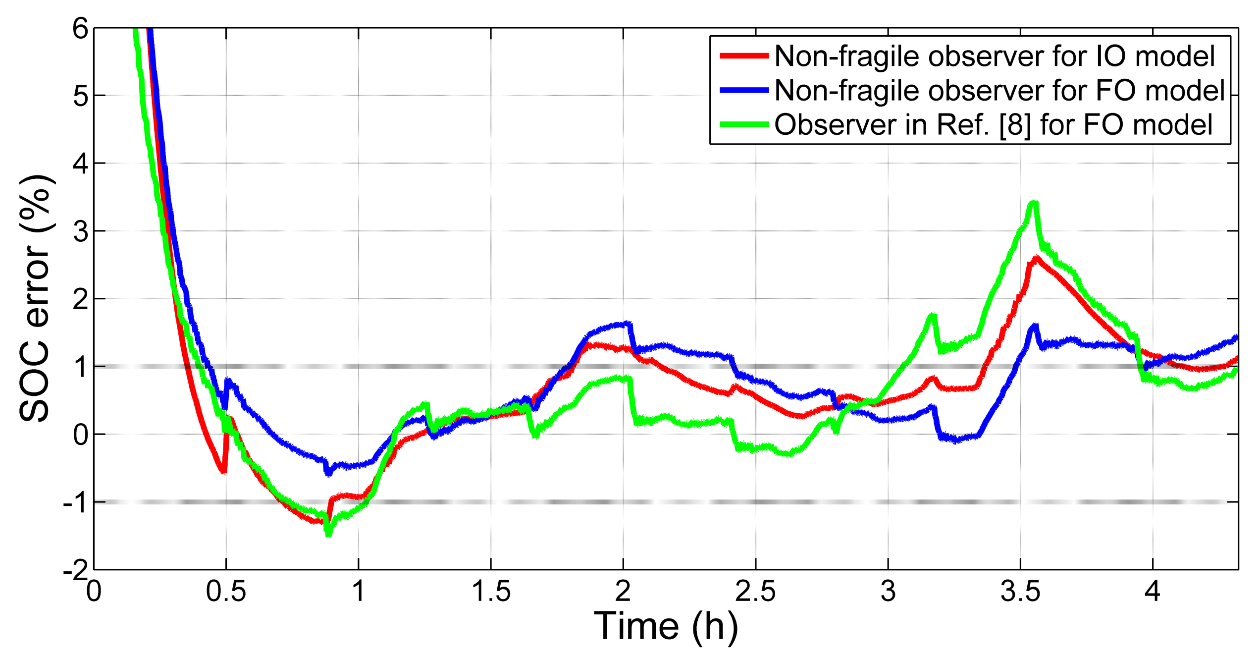
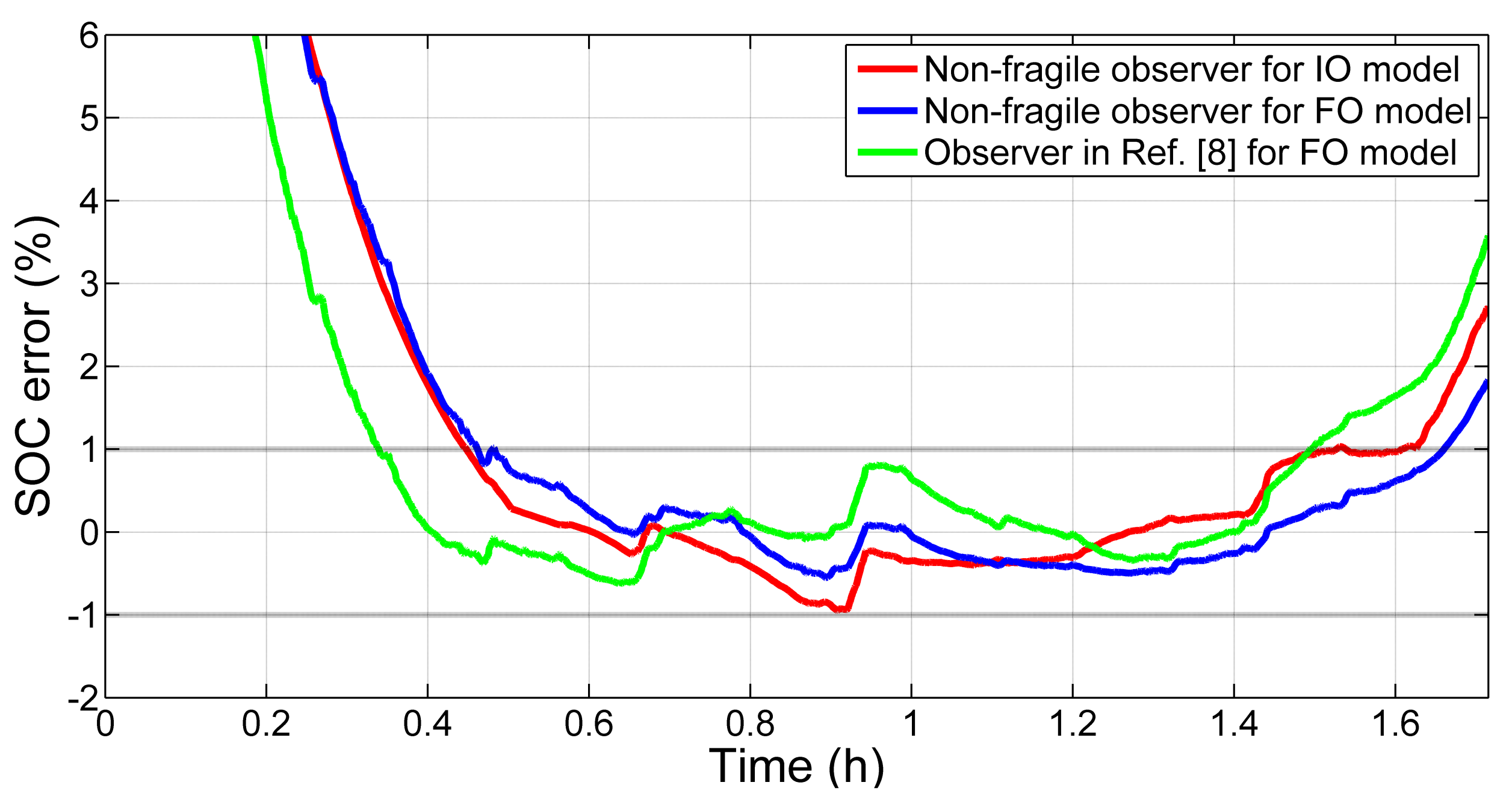
Figure 8. SOC estimation error profiles for UDDS.

5.3.2. NEDC

The current and terminal voltage profiles are shown in Figure 9. The SOC estimation profiles and the SOC estimation error profiles are shown in Figure 10 and Figure 11, respectively.

Figure 9. Current and terminal voltage profiles of NEDC.

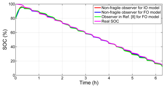
Figure 10. SOC estimation profiles for NEDC.

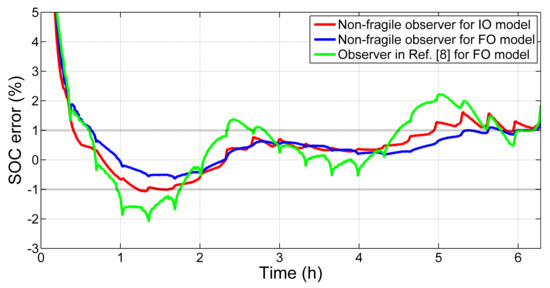
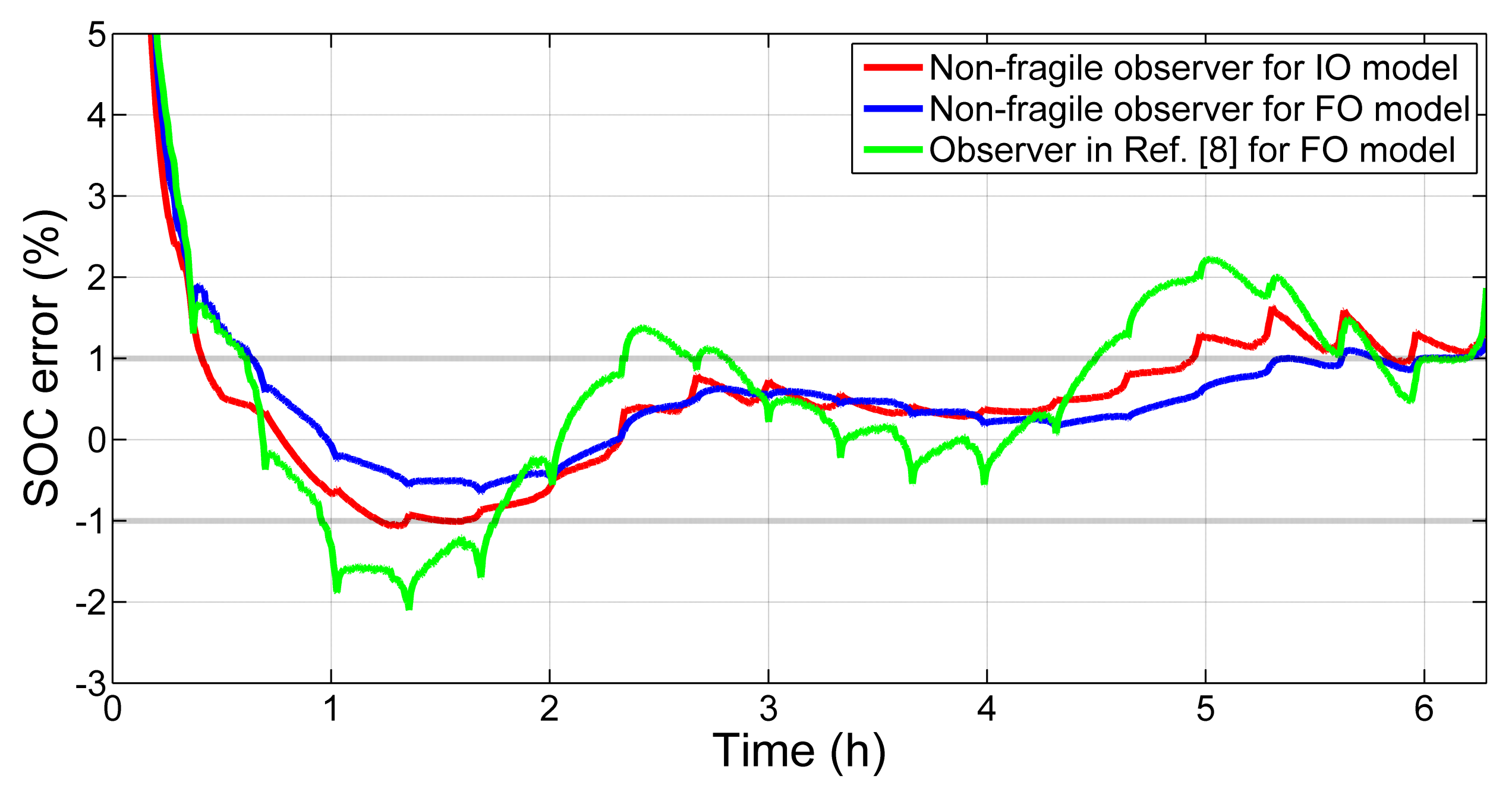
Figure 11. SOC estimation error profiles for NEDC.

5.3.3. HWFET

The current and terminal voltage profiles are shown in Figure 12. The SOC estimation profiles and the SOC estimation error profiles are shown in Figure 13 and Figure 14, respectively.

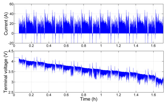
Figure 12. Current and terminal voltage profiles of HWFET.

Figure 13. SOC estimation profiles for HWFET.

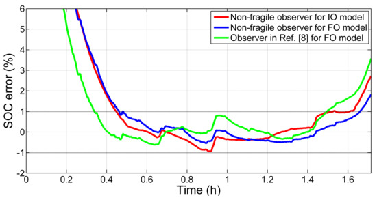
Figure 14. SOC estimation error profiles for HWFET.

5.4. SOC Estimation Results and Evaluation

In order to better discuss the effectiveness of the proposed method under various dynamic conditions, we will display the mean/maximum errors after overcoming the initial SOC error in the following table.

After that, by observing Figure 8, Figure 11 and Figure 14 and Table 2, the following conclusions can be obtained.

• As is shown in Figure 8, Figure 11 and Figure 14 and Table 2 with the initial condition is given as $\left[U_1{U}_{2}SOC\right]$$=[0080\%]$, we draw the conclusion that the SOC estimation accuracy of the proposed observer for the fractional-order battery model is higher than the integer-order battery model. This implies that smaller modeling error brings higher SOC estimation accuracy. This fact is in accordance with the former studies [7,9] in fractional modeling for this battery. Meanwhile, the convergence rate of proposed observer for the battery model is slightly lower than integer-order battery model, which is the main drawback for fractional-order battery with the identified parameters of orders $0<{\alpha }_1,{\alpha }_2<1$.
• In Figure 8, Figure 11 and Figure 14 and Table 2, we can see that the SOC estimation accuracy of proposed observer is superior to the observer in [8]. This is principally because of the Lipschitz constant $\gamma$ mentioned in [8]. The value $\gamma$ is close to 1 in [8] and the SOC estimation error bound is very sensitive to this value as is claimed. Moreover, according to eighth-order fitted curve Equation (8) of the SOC-OCV relationship, the coefficient of linear term of the polynomial is 14.13, which is larger than it in [8]. Moreover, the Lipschitz constant of $U_{\mathrm{OC}}\left(SOC\right)$ function without the linear term is calculated by $\gamma =9.66$, which is much more larger than $\gamma$ in [8] as well. In fact, the fifth-order polynomial used for curve fitting in [8] demonstrates poor accuracy for SOC-OCV relationship of the LiCoO${}_{\mathbf{2}}$ LIB module. Because of the high nonlinearity of SOC-OCV relationship, the observer method in [8] shows lower accuracy below expectation for the battery used in our study. On the contrary, the $H_{\infty }$ performance of the proposed nonlinear observer can deal with the different Lipschitz constant in modeling for various types of batteries, which presents advanced universal property than the observer in [8].
• It is shown in Figure 8, Figure 11 and Figure 14 and Table 2 that the SOC estimation of non-fragile observer Equation (19) shows more accuracy compared to $H_{\infty }$ observer for integer-order model in [5]. This means that, if the gain drifts are taken into account in observer design procedure, the proposed non-fragile observer Equation (19) outperforms the observer in [5]. Therefore, clearly, non-fragile observer functions in tolerating additive perturbation or gain fluctuations on the observer gain. Thus, the proposed non-fragile $H_{\infty }$ observer design criterion can not only restrict the effect of the modeling error and measurement noises on the state estimation, but also limit effect of the gain drifts on observer.

Based on the above analysis, we can see that proposed observer for the fractional-order battery model is more effective than the integer-order battery model. The proposed method can be generally used for SOC estimation of various types of batteries. The non-fragile observer design criterion is robust under the effects of gain drifts.

6. Conclusions

This paper presents a non-fragile nonlinear observer based on a time-varying gain algorithm which can estimate the SOC of the LIBs in electric vehicles accurately. The fractional 2nd-order RC model compared with integer 2nd-order RC model is introduced to model the charging/discharging behavior of the LIB. Moreover, a least-square method mixed with physical behavior based identification method is proposed for model parameters identification. The OCV–SOC relationship is fitted using the eighth-order polynomial for better consideration of the test battery’ property. The principle of $H_{\infty }$ performance design criterion is to reduce the effect of the non-Gaussian system and measurement noises. Furthermore, a non-fragile observer design criterion is proposed to tolerate observer gain drifts to achieve a robust SOC estimation algorithm. Three operation conditions are applied to evaluate the performance of the proposed method by comparing with one former study. Experimental SOC estimation results and evaluation reveal the superiority of the proposed method.

In our study, by comparing the SOC estimation accuracy of fractional-order and integer-order, we reinforce impression that the influence of modeling error is much larger than the measurement noise. As is shown in the parameters identification section, the parameters changes rapidly in low SOC range due to the serious polarization effects. Therefore, despite of the better considering of fractional-order modeling, our future research is towards modeling and online parameters identification in low SOC range.

References

- Ehsani, M.; Gao, Y.; Gay, S.E.; Emadi, A. Modern Electric, Hybrid Electric, and Fuel Cell Vehicles; CRC Press: Boca Raton, FL, USA, 2005. [Google Scholar]
- Li, X.; Yuan, C.; Li, X.; Wang, Z. State of health estimation for Li-Ion battery using incremental capacity analysis and Gaussian process regression. Energy 2020, 190, 116467. [Google Scholar] [CrossRef]
- Tian, Y.; Xia, B.; Sun, W.; Xu, Z.; Zheng, W. A modified model based state of charge estimation of power lithium-ion batteries using unscented Kalman filter. J. Power Sources 2014, 270, 619–626. [Google Scholar] [CrossRef]
- Li, Z.; Xiong, R.; Mu, H.; He, H.; Wang, C. A novel parameter and state-of-charge determining method of lithium- ion battery for electric vehicles. Appl. Energy 2017, 207, 361–371. [Google Scholar] [CrossRef]
- Zhu, Q.; Xiong, N.; Yang, M.; Huang, R.; Hu, G. State of Charge Estimation for Lithium-Ion Battery Based on Nonlinear Observer: An H∞ Method. Energies 2017, 10, 679. [Google Scholar] [CrossRef] [Green Version]
- Monje, C.A.; Gao, Y.; Gay, S.E.; Emadi, A. Fractional-Order Systems and Controls: Fundamentals and Applications; Springer: Berlin/Heidelberg, Germany, 2010. [Google Scholar]
- Xu, J.; Mi, C.C.; Cao, B.; Cao, J. A new method to estimate the state of charge of lithium-ion batteries based on the battery impedance model. J. Power Sources 2013, 233, 277–284. [Google Scholar] [CrossRef]
- Wang, B.; Liu, Z.; Li, S.E.; Moura, S.J.; Peng, H. State-of-Charge Estimation for Lithium-Ion Batteries Based on a Nonlinear Fractional Model. IEEE Trans. Control. Syst. Technol. 2016, 25, 3–11. [Google Scholar] [CrossRef]
- Liu, C.; Liu, W.; Wang, L.; Hu, G.; Ma, L.; Ren, B. A new method of modeling and state of charge estimation of the battery. J. Power Sources 2016, 320, 1–12. [Google Scholar] [CrossRef]
- Xiao, R.; Shen, J.; Li, X.; Yan, W.; Pan, E.; Chen, Z. Comparisons of modeling and state of charge estimation for lithium-ion battery based on fractional order and integral order methods. Energies 2016, 9, 184. [Google Scholar] [CrossRef]
- Zhong, F.; Li, H.; Zhong, S.; Zhong, Q.; Yin, C. An SOC estimation approach based on adaptive sliding mode observer and fractional order equivalent circuit model for lithium-ion batteries. Commun. Nonlinear Sci. Numer. Simul. 2014, 24, 127–144. [Google Scholar] [CrossRef]
- Zhong, Q.; Zhong, F.; Cheng, J.; Li, H.; Zhong, S. State of charge estimation of lithium-ion batteries using fractional order sliding mode observer. ISA Trans. 2016, 66, 448–459. [Google Scholar] [CrossRef]
- Xia, B.; Chen, C.; Tian, Y.; Sun, W.; Xu, Z.; Zheng, W. A novel method for state of charge estimation of lithium-ion batteries using a nonlinear observer. J. Power Sources 2014, 270, 359–366. [Google Scholar] [CrossRef]
- Liu, L.; Wang, L.Y.; Chen, Z.; Wang, C.; Lin, F.; Wang, H. Integrated system identification and state-of-charge estimation of battery systems. IEEE Trans. Energy Convers. 2013, 28, 12–23. [Google Scholar] [CrossRef]
- Lin, C.; Mu, H.; Xiong, R.; Shen, W. A novel multi-model probability battery state of charge estimation approach for electric vehicles using H-infinity algorithm. Appl. Energy 2016, 166, 76–83. [Google Scholar] [CrossRef]
- Zhang, F.; Liu, G.; Fang, L.; Wang, H. Estimation of battery state of charge with H∞ observer: Applied to a robot for inspecting power transmission lines. IEEE Trans. Ind. Electron. 2012, 59, 1086–1095. [Google Scholar] [CrossRef]
- Ibrahima, N.; Taous-Meriem, L.K.; Mohamed, D. H∞ Adaptive observer for nonlinear fractional-order systems. Int. J. Adapt. Control. Signal Process. 2017, 31, 314–331. [Google Scholar] [CrossRef]
- Heleschewitz, D.; Matignon, D. Diffusive Realisations of Fractional Integrodifferential Operators: Structural Analysis under Approximation. In IFAC Proceedings Volumes; Elsevier: Amsterdam, The Netherlands, 1998; Volume 31, pp. 227–232. [Google Scholar]
- Trigeassou, J.C.; Maamri, N.; Sabatier, J.; Oustaloup, A. A Lyapunov approach to the stability of fractional differential equations. Signal Process. 2010, 91, 437–445. [Google Scholar] [CrossRef]
- Boroujeni, E.A.; Momeni, H.R. Non-fragile nonlinear fractional order observer design for a class of nonlinear fractional order systems. Signal Process. 2012, 92, 2365–2370. [Google Scholar] [CrossRef]
- Zhang, L.; Hu, X.; Wang, Z.; Sun, F.; Dorrell, D.G. Fractional-order modeling and State-of-Charge estimation for ultracapacitors. J. Power Sources 2016, 314, 28–34. [Google Scholar] [CrossRef]
- Waag, W.; Fleischer, C.; Uwe, D. Critical review of the methods for monitoring of lithium-ion batteries in electric and hybrid vehicles. J. Power Sources 2014, 258, 321–339. [Google Scholar] [CrossRef]
- Dorato, P. Non-fragile controller design: An overview. In Proceedings of the American Control Conference, Philadelphia, PA, USA, 26 June 1998; pp. 2829–2831. [Google Scholar] [CrossRef]
- Boroujeni, E.A.; Momeni, H.R. An iterative method to design optimal non-fragile H∞ observer for Lipschitz nonlinear fractional-order systems. Nonlinear Dyn. 2015, 84, 1801–1810. [Google Scholar] [CrossRef]
- Sakthivel, R.; Anbuvithya, R.; Mathiyalagan, K.; Prakash, P. Combined H∞ and passivity state estimation of memristive neural networks with random gain fluctuations. Neurocomputing 2015, 168, 1111–1120. [Google Scholar] [CrossRef]
- Wang, J.; Lu, J.; Li, C. Observer-based robust stabilisation of a class of non-linear fractional-order uncertain systems: An linear matrix inequalitie approach. IET Control. Theory Appl. 2012, 2757–2764. [Google Scholar] [CrossRef]
- Mathiyalagan, K.; Park, J.H.; Jung, H.Y.; Sakthivel, R. Non-fragile Observer-Based H∞ Control for Discrete-Time Systems Using Passivity Theory. Circuits Syst. Signal Process. 2015, 34, 2499–2516. [Google Scholar] [CrossRef]
- Zhou, K.; Doyle, J.C.; Keith, G. Robust and Optimal Control; Prentice-Hall: Hoboken, NJ, USA, 1996. [Google Scholar]
- Gao, L.; Jiang, X.; Wang, D. Observer-based robust finite time H∞ sliding mode control for Markovian switching systems with mode-dependent time-varying delay and incomplete transition rate. ISA Trans. 2015, 61, 29–48. [Google Scholar] [CrossRef] [PubMed]
- Kochowski, S.; Nitsch, K. Description of the frequency behaviour of metal-SiO2-GaAs structure characteristics by electrical equivalent circuit with constant phase element. Thin Solid Films 2002, 415, 133–137. [Google Scholar] [CrossRef]
- Westerlund, S.; Ekstam, L. Capacitor theory. IEEE Trans. Dielectr. Electr. Insul. 1994, 1, 826–839. [Google Scholar] [CrossRef]
- Sabatier, J.; Agrawal, O.P.; Tenreiro Machado, J.A. Advances in Fractional Calculus; Springer: Berlin/Heidelberg, Germany, 2007. [Google Scholar]
- He, H.; Zhang, X.; Xiong, R.; Xu, Y.; Guo, H. Online model-based estimation of state-of-charge and open-circuit voltage of lithium-ion batteries in electric vehicles. Energy 2012, 39, 310–318. [Google Scholar] [CrossRef]
- Boyd, S.; Ghaoui, L.E.; Feron, E.; Balakrishnan, V. Linear Matrix Inequalities in System and Control Theory; SIAM: Philadelphia, PA, USA, 1994. [Google Scholar]
- Mu, H.; Xiong, R.; Zheng, H.; Chang, Y.; Chen, Z. A novel fractional order model based state-of-charge estimation method for lithium-ion battery. Appl. Energy 2017, 384–393. [Google Scholar] [CrossRef]
Publisher’s Note: MDPI stays neutral with regard to jurisdictional claims in published maps and institutional affiliations. |
© 2021 by the authors. Licensee MDPI, Basel, Switzerland. This article is an open access article distributed under the terms and conditions of the Creative Commons Attribution (CC BY) license (https://creativecommons.org/licenses/by/4.0/).