Article

A Critical Perspective on Positive Energy Districts in Climatically Favoured Regions: An Open-Source Modelling Approach Disclosing Implications and Possibilities

1
Instituto Tecnológico de Canarias, Departamento Energías Renovables, Playa de Pozo Izquierdo s/n, Santa Lucía de Tirajana, 35119 Gran Canaria, Spain
2
Energy Economics Group, Institute of Energy Systems and Electrical Drives, Technische Universität Wien, Gusshausstraße 25-29/370-3, A-1040 Vienna, Austria
*
Author to whom correspondence should be addressed.
Energies 2021, 14(16), 4864; https://doi.org/10.3390/en14164864
Submission received: 7 July 2021 / Revised: 30 July 2021 / Accepted: 3 August 2021 / Published: 9 August 2021

Abstract

:
Urban areas have been responsible for the majority of the European Union (EU)-wide primary energy demand and C O 2 emissions. To address this issue, the European Union introduced the concept of Positive Energy Districts (PEDs). PEDs are required to have an annual positive primary energy balance. However, if directly addressed in the literature, this energy balance only includes annually fixed primary energy factors and often neglects grid impacts. To bridge this gap, this work proposes a mathematical optimisation approach for PEDs, working towards an open-source model. The model’s main novelty is an hourly primary energy balance constraint. The performed case study on the island La Palma for both an urban and a rural neighbourhood show that the PED concept has a higher net present value (NPV) than solely buying electricity from the grid in all feasible cases. Depending on the space available for PV installations, the NPV increases between 29 and 31% and 25–27% for the rural and urban PED scenarios, respectively. However, in the scenarios with reduced grid impact, the NPV decreases due to the expensive battery installations. Comparing the significantly fossil-based electricity grid mix of La Palma with the renewable-based one of El Hierro shows that the primary energy-based optimisation has more room for flexibility in the high renewable mix. While the dynamic primary energy balance constraint appears promising for operational optimisation, the allocation of correct primary energy factors is crucial.

1. Introduction

In the European Union (EU), approximately 70% of the primary energy demand is in urban areas, and about 90% of the global energy demand increase will take place in cities [1]. Additionally, around 75% of global C O 2 emissions originate from the urban environment [2]. On the other hand, cities play a minimal role in energy generation, particularly from renewable sources [3]. Thus, the working group of the Strategic Energy Technology (SET) Plan regarding action 3.2 “Smart Cities and Communities” established the goal of having 100 Positive Energy Districts (PEDs) within the planning, development or operation stage by 2025 for a more sustainable urban evolution [4]. The European Commission (EC) launched the SET Plan in 2007 to gain a leading role in sustainable energies, focusing on renewable energy generation, storage, flexibility and energy efficiency, among other themes. Those were translated into specific working groups in 2017, with Positive Energy Districts among them [5]. A PED is defined as a community that locally generates more energy from renewable sources than it consumes from the grid on an annual basis while maintaining a net-zero C O 2 emission balance. While this is the main constraint, further focus is laid on system flexibility, and resilience, energy efficiency in buildings, life quality, inclusiveness and sustainability [4,6]. Furthermore, in [7], the authors distinguish spatially between autonomous, dynamic and virtual PEDs. Autonomous and dynamic PEDs have clear spatial boundaries. While the autonomous PED can only export energy, the dynamic PED can freely interchange energy with the distribution grid. A virtual PED extends the spatial boundaries and allows for renewable energy generation outside of the community borders. In this work, the focus is laid on dynamic PEDs.

1.1. Positive Energy District Analysis in Literature

To date, little work has been conducted on the techno-economic analysis of PEDs, considering the annual positive energy balance. In [8], the authors optimise Energy Positive Neighbourhoods (EPN) that are very close to PEDs. They include electricity and heating demand and distinguish between a centralised, single ownership neighbourhood approach and a hierarchical two-level optimisation. The annual energy balance is not described mathematically. In [9,10], specific districts in Vienna are analysed regarding their feasibility to become a PED. The authors use 3-D building models to be fed into the software PVsites for energy generation assessment to establish if they can cover the demand. As a result of this, the Floor Space Index (FSI) is determined to be a crucial factor in densely populated areas for PED feasibility. Only in the case of unrealistic PV roof coverage, an annual positive energy balance was possible but not economically feasible. Thus, a correction factor, considering the FSI, is proposed by the authors. In [11], a calculation approach for the PED energy balance using constant primary energy factors for technology or the grid over a year is proposed. The methodology has not been validated yet. In [12], the authors define assessment criteria for near-zero and positive energy communities. A case study for a newly constructed positive energy community and a renovation based near-zero energy community is conducted using pre-existing software (RETScreen, EnergyPLAN). An integrated energy balance as a constraint is not included, and predefined technology portfolios are compared. Similarly, [13] proposes key performance indicators (KPIs) for energy positive neighbourhoods leading to an energy positivity label. The Excel-based tool “AtLas” is presented to assess the energy positivity of a neighbourhood for long-term planning. [14] proposes a combination of the two software solutions TRANSYS and MOBO (Multi-Objective Building Performance Optimisation) to analyse positive energy communities. The imported electricity and lifecycle cost is optimised simultaneously.
In [15], the authors compare an Excel rule-based and a linear programming optimisation approach for the assessment of self-sufficient districts. Generation, conversion and storage technology is included to supply electricity and heating demand, while minimising the life cycle cost. The authors include a specific constraint for energy self-sufficiency in the model but none is described for energy positivity. The study concludes that major investments in storage can be saved if dynamic PEDs are targeted rather than 100% self-sufficient districts. Judging from available literature regarding techno-economic analyses of PEDs, there is a gap of a specific PED analysis framework focusing on the positive primary energy balance. Additionally, due to the public interest in PED research, there is need for turning this analysis framework into an openly accessible modelling tool. The public relevance of PED research is underlined by the Annex 83, which is a working group of the International Energy Agency Energy in Buildings and Communities (IEA EBC) Programme focusing on PEDs. One specific task of the Annex 83 is the development and identification of modelling tools for PED simulation and optimisation, supporting the design and operation of PEDs [16].

1.2. Annual Energy Balance in Energy System Modelling

As literature about PED energy system modelling is quite rare, the very similar concept of zero energy district, community, neighbourhood or building is investigated to understand the current approach towards the annual energy balance. In terms of energy balance modelling, PEDs and the related zero energy concepts are almost equal. While PEDs have to generate more energy annually than consume, zero-energy concepts have to generate as much as they consume on an annual basis. The delta of the excess consumption is not defined and therefore, could be insignificantly small. Thus, the approach towards annual energy balancing integrated in energy system modelling would be very similar. In the literature, (nearly) zero energy concept analysis and techno-economic modelling is approached in two ways: without and with a model-integrated balance as a constraint Model-integrated means that the energy balance is explicitly part of the optimisation model in form of a constraint. Regarding the first method, without explicit constraint, [17] presents an approach that integrates demand and supply side improvements for net-zero energy districts. The work considers grid impacts as specific as voltage violations and power backfeeding. Different PV and storage technology portfolios are tested to determine those solutions that fulfil the net-zero energy district goal annually and even work towards it on a 15-min resolution basis. In [18], the authors published a multi-objective goal programming approach to assess different strategies towards net-zero energy communities. The case study community does not achieve the net-zero energy community goal, which is not implemented as a constraint. Similarly, the case study in [19] compares the primary energy demand and generation after tailored retrofitting of a castle with various tools, to realize the achievement of a net-zero energy building. Other studies apply the same way of comparing local generation and demand after the optimisation. While this is one way to evaluate if an urban development project achieves net-zero or positive energy status, it does not allow the model to optimise the technology portfolio and the dispatch having the energy balance goal in mind.
In [20], the authors elaborate a mathematical optimisation model for nearly zero energy buildings that is subject to the constraint of achieving an annual energy match ratio of 95–100%. This forces the result to at least achieve a nearly zero-energy building status. The authors of [21] use a multi-objective, heuristic optimisation approach for the analysis of a net-zero energy building, specifically including the balance as a constraint. Primary energy is not considered to value electricity generation differently. Finally, in [22], the authors present a mixed-integer linear programming (MILP) approach for specifying the cost and optimal energy system design of zero energy buildings. A primary energy balance and a zero-emission constraint are included in the model. According to existing literature, there are only few studies with a primary energy balance integrated as a constraint in the modelling approach. No study considers hourly primary energy changes of the electricity mix. This would be important for operational optimisation, as in reality, the grid generation mix is not constant but can vary drastically between high renewable shares and high fossil shares, depending on the installation capacity and renewable resources such as sun and wind. A PED should provide the additional flexibility to respond to those different grid mix constellations. A dynamic assessment of the grid’s primary energy factor integrated in the optimisation model could be one approach to achieve this. While a PED shall increase the share of renewable energy generation locally, it should also provide resilience to the grid. Grid stability, however, is often neglected in the literature.

1.3. Open-Source Energy Modelling

As elaborated extensively in [23], energy system models often are hardly understandable to third parties due to their black-box approach. However, this conservative approach towards modelling due to a variety of potential concerns makes reproducibility and credibility of results barely possible [24]. Recently this has become subject to change, and globally, more and more open-source energy system modelling approaches are getting published under respective open-license agreements [25]. The open energy modelling initiative lists more than 50 open-source energy modelling approaches, classified according to indicators such as energy sectors, model type, or time-/geo-resolution [26]. In order to contribute to this movement, the modelling approach presented in this work will be released as an open-source model. For this paper, the model and case-study data is provided under [27]. Access will be further improved to match the FAIR criteria of Findability, Accessibility, Interoperability, and Reusability [28].

1.4. Progress beyond the State of the Art

This paper contributes to the state of the art in two significant ways: Firstly, this work discusses perspectives of Positive Energy Districts that go beyond the annual positive energy balance using the case study approach. This includes the problem of available space for local renewable energy generation, particularly in urban areas, which is the target zone of the concept. Therefore, a rural area is compared with an urban one in climatically very advantageous conditions (a high renewable energy potential and predominant electricity demand; no heating and cooling needed), which favour the creation of PEDs. Furthermore, the distribution grid impact is examined. While it might be possible to supply more than the annual energy demand from local and renewable resources, how this energy is supplied and exchanged with the grid is of major importance to actually add value to the entire energy system instead of straining it.
Secondly, and most importantly, the paper introduces an electricity import and export mechanism based on hourly changing primary energy factors of the grid according to its current technology mix. This novel approach in energy system planning and scheduling is tailored explicitly for district concepts that are constrained by a primary energy balance such as the PED and aims to provide flexibility in two ways. On the one hand, the dynamic mechanism provides flexibility to the district concept itself. The district scheduling can consider times with high grid mix primary energy intensity for export and low grid energy intensity for import. Thus, the district reduces its primary energy export requirements over the year and, therefore, also the need for expensive technology investment. On the other hand, this dispatch behaviour would also add flexibility to the surrounding grid. Considering that the grid primary energy factor is high during low renewable generation and vice versa, district electricity export during high primary energy grid mixes and import during low ones can stabilise the grid. This work demonstrates the potential of primary energy arbitrage in PEDs and discusses its possibilities beyond the PED scope for island systems that do not have their own electricity market. Finally, by adding this approach to energy system planning and scheduling, primary energy intensity gets reduced, which contributes to one of the primary goals of the European Union in the energy transition, namely increasing energy efficiency [29].
The specific research questions that this work aims to answer therefore are the following:
  • Is a PED technically and spatially feasible under perfect climatic conditions?
  • How is a PED affected by the type of settlement (urban or rural) under these conditions?
  • What are the PED’s implications in terms of cost and technology portfolio if the grid impact is kept low?
  • How does the renewable share of the grid mix affect the PED economically and technically, if assessed hourly?
To answer these research questions, the paper is structured as follows: Section 2 is the Methodology, including an overview of the proposed PED model, its mathematical description and the narration of the case study. Section 3 presents and discusses the case study results and Section 4 shows the work’s conclusions and proposals for future work.

2. Materials and Methods
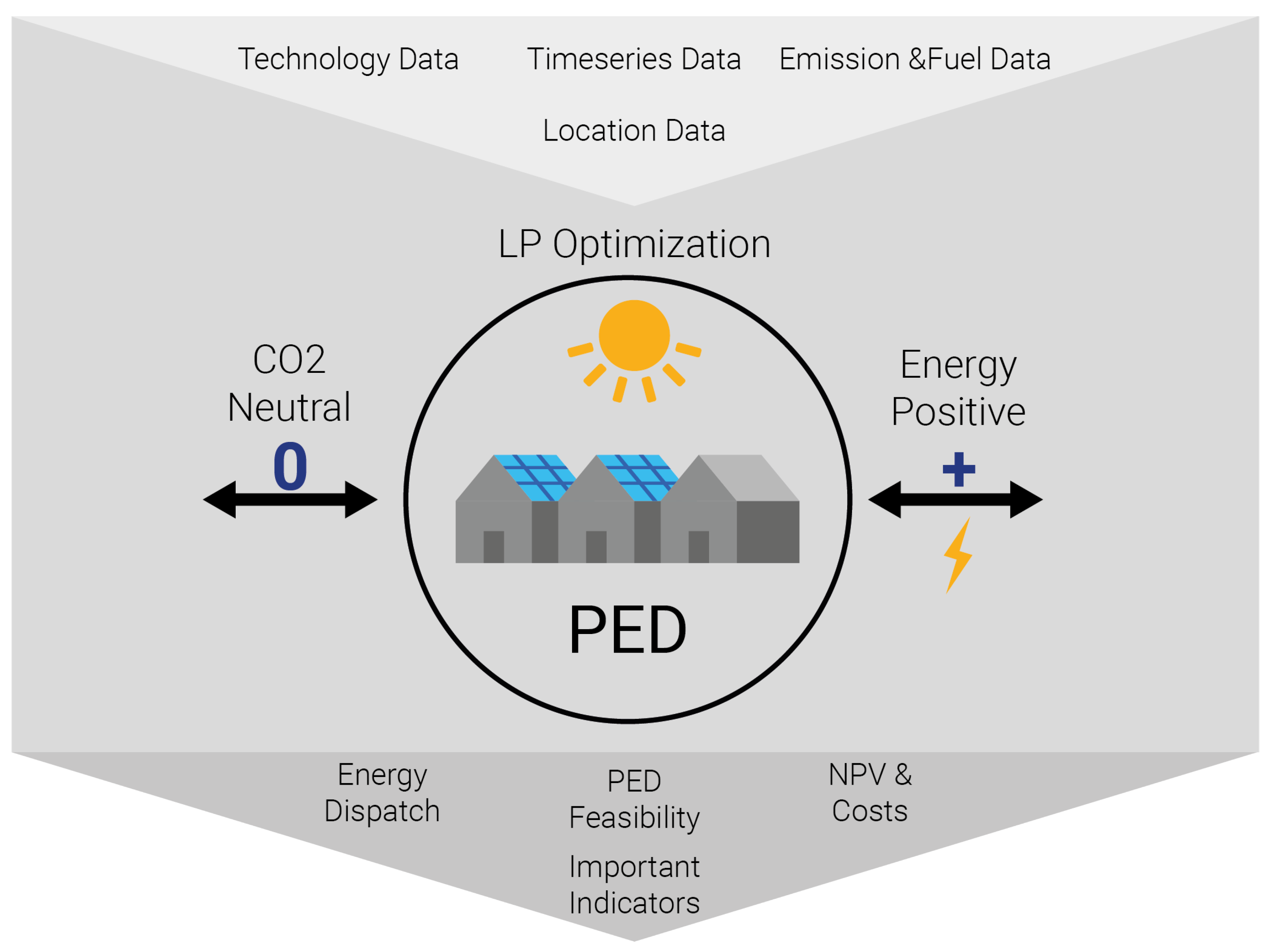
This section introduces the PED modelling framework developed from scratch. Due to its importance, first the novel energy balance is defined in Section 2.1, followed by the mathematical formulation in Section 2.2, and finally the applied case study in Section 2.3.

2.1. Model Overview

Figure 1 gives an overview of the tailor-made modelling framework for PED analysis. The linear programming model itself is written in Python, using the well-known Pyomo optimisation package [30,31]. Inputs in the model are of 4 major subtypes as illustrated in Figure 1. Technology data includes the selected technologies for optimisation alongside their costs and additional data such as efficiencies. Timeseries data encompasses all time-dependent empirical data such as the load(s), grid tariffs, meteorological data and grid generation data. Emission and Fuel data refers among others to C O 2 costs and factors of the grid and technologies. Location data refers to the geographical location of the planned PED. This includes available space for PV installations and pre-existing PV systems. Finally, it can be specified what kind of PED balance shall be considered as well as the time-resolution, time horizon and interest rate. Static and dynamic primary energy factors of electricity (see Figure 2), as well as the possibility to disable any PED restriction can be chosen for the PED balance.
Major constraints include the PED-relevant requirement of having a positive energy balance as well as local C O 2 neutral energy generation. Furthermore, technological and cost-relevant constraints are included to describe the energy system. This work focuses on electricity as the only energy type, justified by the demand of the case study location. Outputs of the model include the technical feasibility of a PED development given the spatial constraints, the NPV and its cost components of the optimal solution, as well as the optimal energy dispatch and other relevant indicators such as the grid export and import power.
The core and novelty of the PED model framework is its energy balance restrictions that define the PED concept as elaborated in Figure 2. To compare different forms of energy such as electricity and fuels, primary energy is taken as an indicator. The model framework allows using a static or dynamic approach to derive the PEF for the positive energy balance. The static energy balance applies a constant primary energy factor (PEF) depending on the local electricity grid mix. When electricity is imported, it is multiplied with the grid mix specific PEF to account for its generation. Electricity in the PED is only allowed to be of renewable sources. According to the non-renewable only calculation method, renewably generated electricity will not be accounted for [32]. Thus, to acknowledge this in the export-electricity, a balance mechanism is applied, and renewable export electricity is treated as avoided electricity generated by the grid mix. Therefore, exported power is also valued with the PEF of the grid mix. The static approach does not require high-resolution generation mix time-series data. However, if these data are available, the dynamic approach can be taken. Here, each time step is considered individually by looking at the marginal cost curve of the generation mix at this exact time step. Exported energy reduces the demand as depicted with Δ Demand in Figure 2. Therefore, at each time step, the PEF of the most expensive generation technology replaced by the PED export can be taken. For the import to cover the electric load, the average PEF of the current generation mix is taken. It is crucial that for other electricity import, which does not cover the electric load (e.g., powerflow grid to battery) the PEF of the most expensive technology of the marginal cost curve is taken. This is further elaborated in Appendix A. This dynamic behaviour gives the model the freedom to increase value of electricity export and import above the plainly monetary indicator of tariffs.

2.2. Mathematical Model

The following section describes the mathematical formulation of the developed linear programming model. Model optimisation variables and parameters are depicted in Table 1. The model decision variables are determined by the optimisation, while the remaining model parameters have to be given as an input to the model.

2.2.1. Objective Function

The general objective of the model is the maximisation of the net present value (NPV) over a given time horizon Y, usually 20 years. This gives an indication of the financial feasibility of a PED project if planned holistically by, e.g., a city council or municipality. Thus, practical relevance in early stage city-planning is given. The respective mathematical formulation is given in Equation (1). The NPV is determined by:
  • I 0 , the initial investment cost in year zero of the optimised technology portfolio;
  • R y , the annual revenues from selling excess generated electricity to the grid; specified in Equation (2);
  • C y , the overall annual OPEX, which is composed out of fixed and variable annual cost, shown in Equations (3) and (4), respectively.
max v V N P V = max v V ( I 0 + y = 1 Y ( R y C y ) ( 1 ( 1 + i ) y ) )
R y = t s T S x X p y , t s x , g r i d d t 60 f e e d i n y , t s
O & M _ f i x y = t e c T E C c a p t e c O & M _ f i x t e c
O & M _ v a r y = t e c T E C t s T S z Z ( p y , t s t e c , z O & M _ v a r t e c ) + t s T S z Z ( p y , t s g r i d , z d t 60 t a r i f f y , t s )
With v—optimisation variable, V—vector of optimisation variables, y—year, Y—time horizon, i—interest rate, t s —time step, T S —number of time steps in one year, x—“technology” with electricity output, X—Vector over “technologies” with electricity output, d t —the time resolution in minutes, d t 60 —share of hour [h], f e e d i n y , t s —the feed-in tariff at each ts each year, t e c —specific technology, T E C —vector of technologies selected, c a p t e c —the capacity of each technology [kW or kWh], z—electricity input “technology” (including load), Z—vector over electricity input “technologies”, and p y , t s x , z —the power flow matrix at each time step from technology x to z [kW].

2.2.2. PED Energy Balance

Positive Energy Districts are determined by their energy balance which thus is of particular importance in this model framework. There are 2 types of PED balance available to choose, depending on the availability of data. If there is high resolution data of the electricity mix of the main grid at each time step the dynamic PED model can be chosen as shown in Equation (6). This means that the primary energy factor is re-evaluated at each time step according to the current electricity grid mix, which adds flexibility to the model as it can take dispatch decisions according to the current primary energy factor. Otherwise the static approach has to be taken as described in Equation (5), where the primary energy factor is equal at each time step. For further explanation of the two balance types refer to Figure 2 and its elaboration. Of course, the electric load needs to be covered at any time as well, as described in Equation (7).
t s T S x X p y , t s x , g r i d d t 60 P E F _ e x > t s T S z Z p y , t s g r i d , z d t 60 P E F _ i m + f u e l _ c o n s y , t s
t s T S x X p y , t s x , g r i d d t 60 P E F _ e x y , t s > t s T S z Z p y , t s g r i d , z d t 60 P E F _ i m z , y , t s + f u e l _ c o n s y , t s
With p y , t s x , g r i d —the power flow matrix at each time step from technology x to the grid [kW], t s —time step, T S —number of time steps in one year, x—“technology” with electricity output, X—Vector over “technologies” with electricity output, d t —the time resolution in minutes, d t 60 —share of hour [h], P E F _ e x —constant primary energy factor of exported electric energy, p y , t s g r i d , z —the power flow matrix at each time step from the grid to technology z [kW], z—electricity input “technology” (excluding load), Z—vector over electricity input “technologies”, P E F _ i m —constant primary energy factor of imported electric energy, P E F _ e x y , t s —dynamic PEF of exported electric energy for each time step, and P E F _ i m y , t s —dynamic PEF of imported electric energy for each time step.
The constant PEFs can for example be both equal to the grid mixes average PEF. The dynamic export P E F _ e x y , t s is calculated as the energy exported times the PEF of the most expensive technology of the grid generation mix at that time step. The dynamic import P E F _ i m y , t s is calculated as the average PEF of all technologies of the grid mix at each given time step if the load is covered. For any other power flow, also the PEF of the most expensive technology of the current marginal cost curve is taken.
l o a d _ e y , t s = x X p y , t s x , l o a d
With l o a d _ e y , t s —electricity load of the district at each times step each year and p y , t s x , l o a d —the power flow matrix at each time step from technology x to the load [kW].

2.2.3. PV Constraints

PV is one of the most important renewable energy generation technologies for PEDs as it can be applied to existing rooftops, carports or bus stations and therefore is in low competition to other ground usage such as living or recreational space which is important in urban areas. To estimate the potential, tilt and azimuth angle of the roofs and therefore the panels are of high importance. PV is separated in PV for flat surface applications and PV for tilted rooftops. Equation (8) describes the PV power generated at each time step each year. For flat surface installations, an azimuth angle of 180° and a tilt angle equal to the location’s latitude is assumed for northern hemisphere installations. For tilted rooftops the angles of the roofs have to be approximated to a predefined set of azimuth and tilt angles to reduce model complexity. Here, eight azimuth and three tilt angles are considered. The area used for PV installation has to be smaller or equal to the free area available as displayed in Equation (9). The total installed peak PV capacity in [ k W p ] under STC conditions is determined as show in Equation (10).
z Z p y , t s p v , z = A a z , β I r r a z , β , y , t s η p v P R
A a z , β A _ a v a i l a z , β G C R
c a p p v = a z A Z β T I L T A a z , β η p v
With p y , t s p v , z —the power flow matrix at each time step from PV to technology z [kW], A a z , β —area (includes existing installations) used for PV with respective azimuth and tilt angle, I r r a z , β , y , t s —tilted irradiance in [kW/m2] for each respective angle constellation and each time step, η p v —efficiency of the PV module and P R —performance ratio of the system installation, that includes unavoidable losses of a PV plant, A _ a v a i l a z , β —area available according to angle constellation and G C R —ground coverage ration, which accounts for spacing of tilted PV installations on flat roofs to avoid shading, c a p p v —installed peak capacity of PV [kW], A Z —vector of used azimuth angles, and T I L T —vector of used tilt angles.
The tilted irradiance has been calculated for each angle pair according to [33] and the model used for solar zenith and azimuth angle at a certain location and time has been derived from [34].

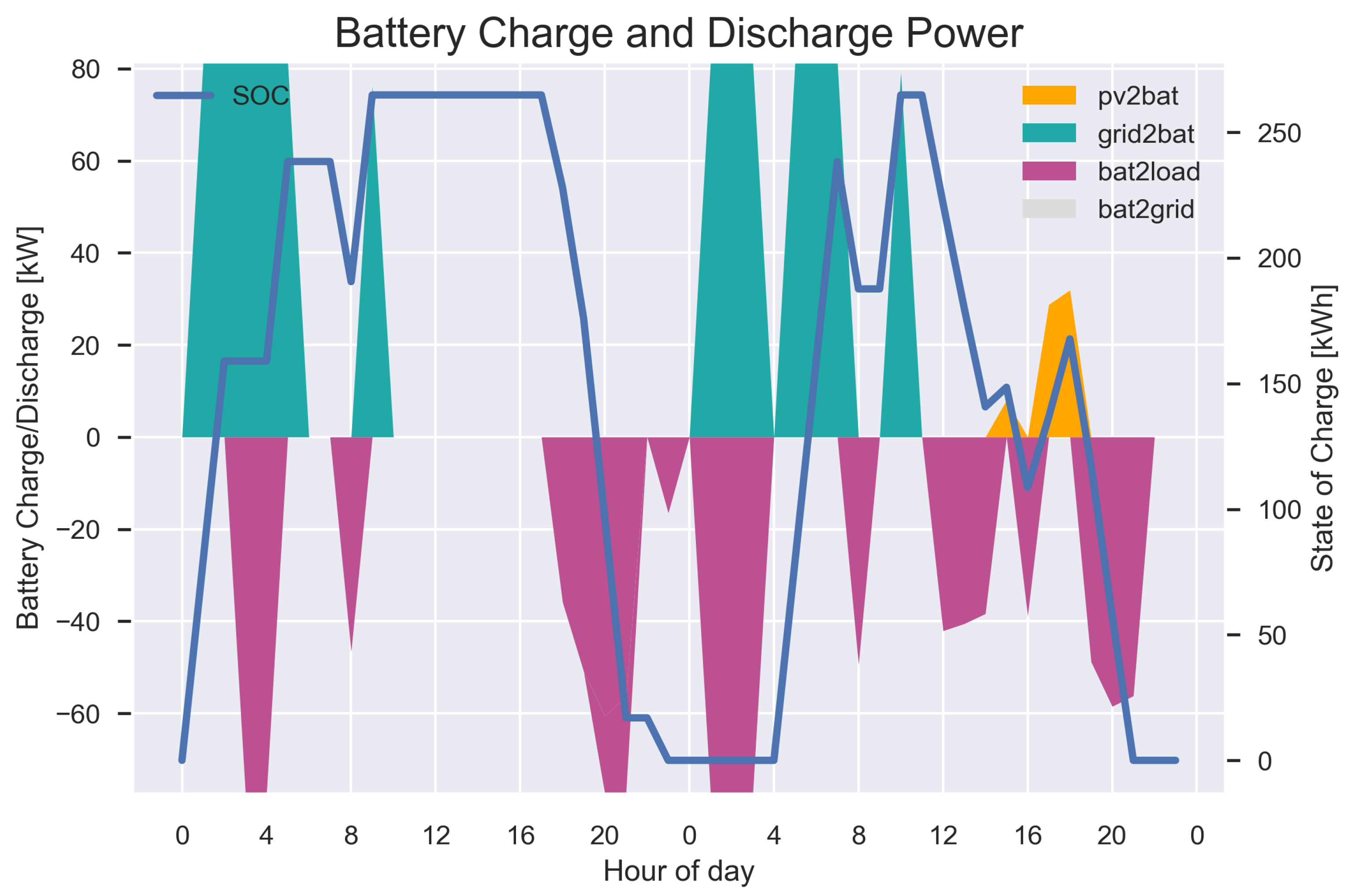
2.2.4. Battery Constraints

Equation (11) shows the battery’s state of charge (SOC) update at each time step. For a smooth connection of horizon years and an initial battery behaviour, if t s = 0 and y = 1 , S O C y , t s is taken and if t s = 0 and y 1 the S O C of the last time step of the previous year. Additionally the S O C is limited to the battery’s capacity at any time as shown in Equation (12) and cannot be lower than 0. The charge and discharge power is limited to a fraction of c a p b a t t e r y that can be defined as an input, as well as the initial S O C 1 , 0 .
S O C y , t s = S O C y , t s 1 + x X p y , t s x , b a t t e r y d t 60 η b a t t z Z ( p y , t s b a t t e r y , z d t 60 ) η b a t t
0 S O C y , t s c a p b a t t e r y
With S O C y , t s —State of Charge of the battery at each time step each year, p y , t s x , b a t t e r y —the power flow matrix at each time step from technology x to the battery [kW] (charging), η b a t t —round-trip efficiency of the battery, p y , t s b a t t e r y , z —the power flow matrix at each time step from the battery to technology z [kW] (discharging), and c a p b a t t e r y —the capacity of the battery [kWh].

2.3. Case Study Definition
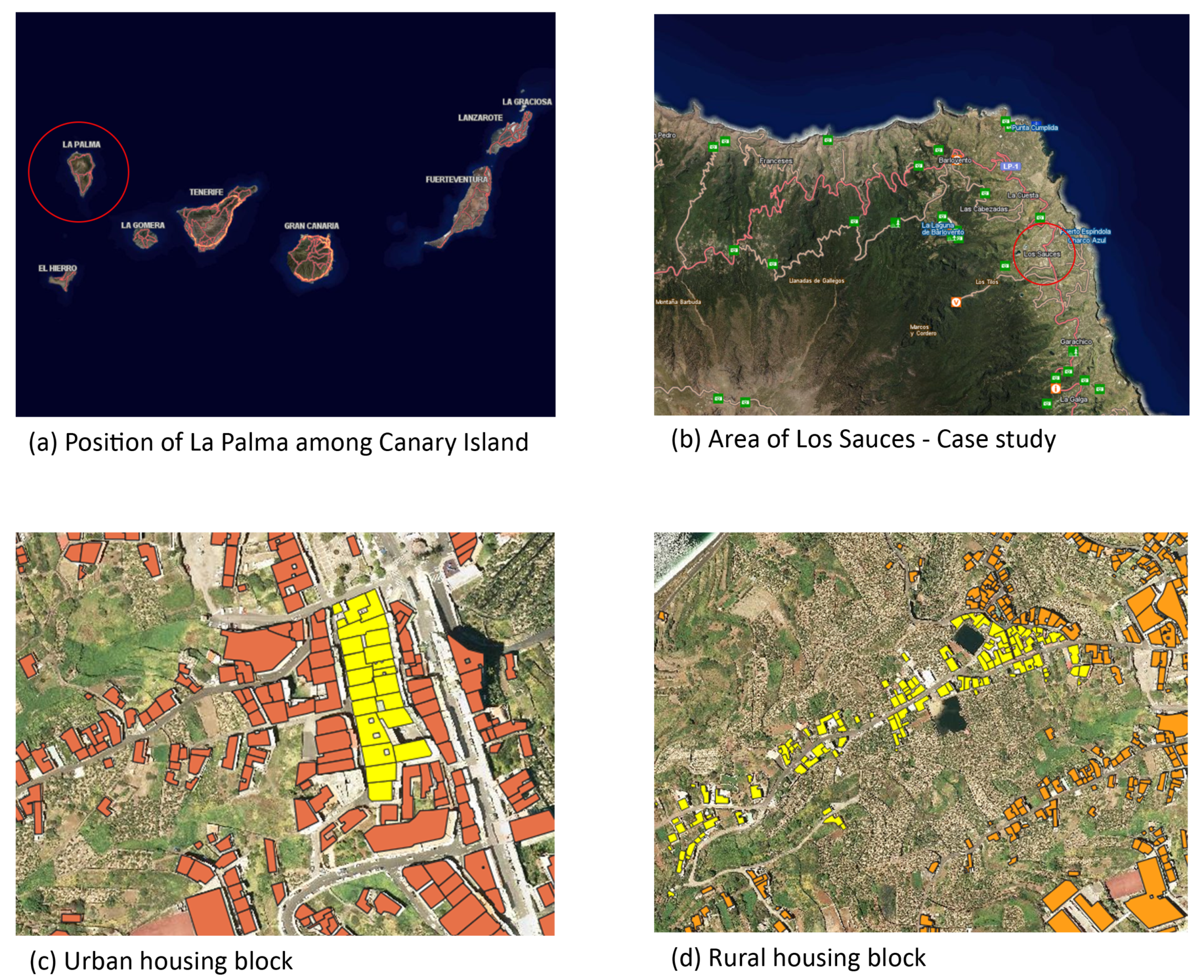
In the following section, the case study on which the model is applied is described. It consists of both an urban and a rural site on the island of La Palma, in the town Los Sauces that are considered for potential PED development. The various location specific input parameters are described and scenarios are defined.

2.3.1. Location

Figure 3 describes the location of the rural and urban test site, which are very close to each other in Los Sauces. La Palma has been selected as an initial case study due to its favourable climate conditions. Those allow to only focus on electricity demand and neglect heating and cooling for now. Furthermore, the islands that are not connected through underwater cables (Gran Canaria, La Palma, El Hierro) can be considered a closed system, making them very interesting from the standpoint of the grid generation mix. The grid generation mix of all islands, except El Hierro, is dominated by fossil fuels, mainly in the form of diesel. Thus, renewable focused projects gain interest in the sun-, and wind-rich archipelago to cut on diesel derived electricity to reduce C O 2 emissions, cost and dependency. Among the Canarian Islands, La Palma is one of those with the least stable grids [35]. Therefore, a PED project that values flexibility would be a worthy addition. Regarding selecting the town of Los Sauces, a local initiative called La Palma Renovable is currently planning the first steps of the island’s energy transition in exactly this location. A floating PV power-based energy community with a 100 kW p installation on a water storage is proposed in the area shown in Figure 3d [36]. This would generate renewable electricity locally and reduce the evaporation of water from the storage. Thus, as the town of Los Sauces is already in the centre of interest for energy communities, this case study is applied there as well.
Both sites have an aggregated gross floor area of approximately 15,800 m2, despite the large difference in surface area. Thus, the floor space index mentioned before as a great indicator of PED feasibility lies around 3 and 0.68 for the urban and rural district, respectively. The gross floor area is derived from the Spanish open kataster data in QGIS. Table 2 and Table 3 show the available space for PV power installations for the urban and the rural district, which has been derived manually in QGIS.

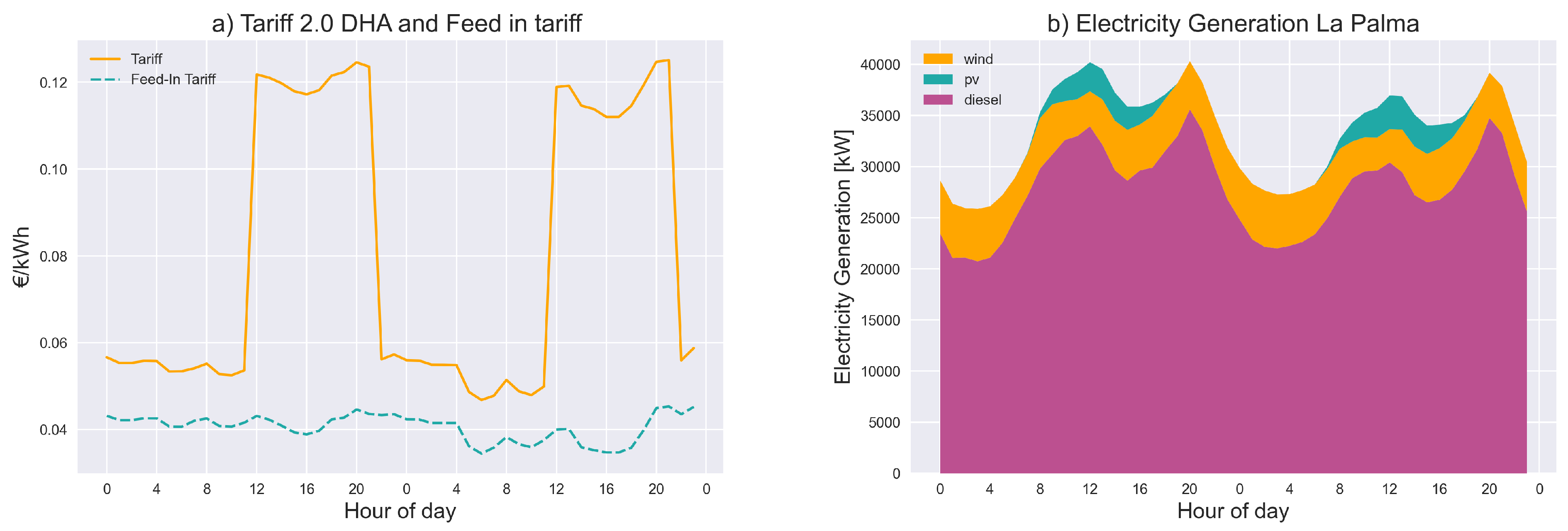
2.3.2. Time Series Data

Time series, location-specific input data include the electricity demand, the tariffs, the grid generation mix and meteorological data. Demand, generation and tariff data are taken for the year 2019 not to be affected by COVID-19. The electricity demand is approximated as a share of La Palma’s electricity demand, considering the gross floor area (GFA) of the district. Since the urban and rural GFA is equal, both districts’ electricity demand is assumed to be similar. The GFA share of all buildings in La Palma is 0.0159%. This value is applied to calculate the hourly demand of both districts. The hourly island-wide load is derived from [37], which is an open data website of the Spanish system operator Red Eléctrica de España (REE). There are two types of dynamic grid tariffs for consumers below 10 kW capacity in Spain (default and two periods; TARIFF 2.0 A and TARIFF 2.0 DHA, respectively), beyond the somewhat static tariffs. The dynamic tariffs, called “voluntary price for the small consumer” (PVPC), represent the cost of electricity generated and are thus very well suited for PED projects supposed to supply flexibility. The PVPC tariff is composed of the day ahead and intraday market price, cost of ancillary services, distribution and transmission tariffs, capacity payments and other fees. Additionally, the PVPC mechanism offers a surplus compensation for PV production according to the electricity generation cost. As this dynamic feed in tariff was introduced the 6 April 2019 by the royal decree 244/2019 [38], the tariff for the beginning of the year is calculated according to the average difference to the default tariff during the rest of the year. The grid tariffs are also derived from [37]. Generation mix data for each island is obtained from [39]. Figure 4 shows a graph of the 2.0 DHA tariff (chosen for this study) as well as the feed-in tariff and of the generation mix during a specific day. Here, the strong dependency on expensive diesel fuel of the island of La Palma becomes very apparent. Meteorological data, such as global horizontal, direct normal and diffuse irradiance, and temperature and wind speed, is taken from [40]. All further necessary data is shown in Appendix B.

2.3.3. Initial Scenarios

This section describes the initial scenarios for the urban and rural PED analysis, which are summed up in Table 4. At first, for comparison, the status quo is calculated. Since there are no pre-existing PV installations and the demand is the same for the urban and rural district, only one status quo scenario is needed for both districts. The status quo scenario will show the cost of doing nothing and therefore the cost of electricity purchase only. Next, for the urban and the rural district, an optimisation is done without the requirement of being a PED allowing for all the area, including terrace and water pond surface for PV power generation. This is then compared to the same optimisation with the requirement of having a positive energy balance, to see if the PED scenario would be the generally preferred solution. As it is pretty unlikely that all of the available space would be used for PV generation because the owners would want to use it otherwise or because they do not want to participate in, e.g., an energy community, an urban and rural scenario where only roof area and potential carport area is used, that has no other possible occupation. The PED status is required in these variations. If any of those two scenarios cannot fulfil the PED requirement sensibly due to space restrictions, 25% of terrace space is allowed for PV panel installations as a third variation scenario.

2.3.4. Sensitivity Scenarios

Beyond the aforementioned variation in space available for PV generation, variation in grid power exchange (PES), grid generation mix (GGS) and grid tariff (GTS) is applied to specific scenarios. The grid power exchange restriction is used for the urban and rural district that uses the least amount of space and fulfils the PED requirement sensibly. Here, the grid connection power is restricted to 2, 1.5 and 1 times the maximal load at a time step, to decrease negative grid impact by the PED. Subsequently, the two aforementioned urban and rural scenarios are tested in a grid mix with very high renewable penetration to evaluate if this has an impact on the PED’s NPV due to the lower primary energy intensity of the grid. Here, the grid mix of El Hierro is used, which had a renewable share of electricity generation of 67% compared to 10% on La Palma in 2019 [35]. Figure 5 shows the generation mix of El Hierro on the 24th and 25th of August in 2019. These two days are chosen because the generation mix of El Hierro is completely renewable at some times, while supported by diesel at other times. This allows for an in-depth assessment of the influence of extreme changes of the grid mixes PEF, as shown in Section 3.3. Overall it can be seen that the electricity generated during this day is mainly renewable wind power that is partly stored by pumped hydro storage to bridge low wind generation. Electricity used for the pumped hydro storage is represented as negative values, while discharging the hydro-basins is shown positively in Figure 5. Finally, it is investigated how a grid tariff increase of 2% (average yearly tariff increase in Europe 2008–2020 [41]) and 4% annually affects scenario S1, urban PED scenario with least space used and with a grid power exchange limit of factor 2. The recently introduced version of the PVPC tariff supports the assumption of an increasing and more fluctuant electricity cost. The PVPC 2.0 TD was introduced on the 31st of May 2021 [42].

3. Results

This section presents the results of the described case study and its sensitivity analysis.

3.1. Rural vs. Urban and Variation of Roof Space Available

Figure 6 illustrates the net present value of each considered scenario as well as its composition by CAPEX, fixed cost, variable cost and revenue from grid sales. Table 5 shows the NPV, optimised technology portfolio for each scenario, as well as the respective electricity export/import ratio and the C O 2 emissions associated with the grid import. In the status quo scenario, no electricity generation is available, and the NPV is solely composed of variable cost, which in this case is the grid tariff only. Since the C O 2 emissions are only associated with the grid mix (time-dependent), S1 has the highest C O 2 emissions. As solar PV is very profitable under the given climate conditions, the rural and urban “no PED” and “PED” scenarios are identical and utilise all of the available area for PV installations. The NPV increases by EUR 150,851 for the rural PED and by EUR 136,696 for the urban equivalent over status quo. For the rural scenario, where no pond or terrace surfaces are considered for PV installations the NPV decreases around EUR 10,000 from the rural scenario where all area is selected, due to decrease solar PV electricity generation. However, the PED solution is still economically superior over the status quo.
On the other hand, in the urban scenario, where rooftop terraces are not considered, a PED is deemed to be infeasible by the optimisation, as not enough area is available for PV power generation. Thus, 25% of terrace usage has been allowed for PV generation in the urban scenario, which has an increased NPV of EUR 125,643 over the status quo scenario. SVS3 has the lowest electricity export/import ratio with 1.04, as it provides the least space for local generation. Among the scenarios with PV systems, it can be seen that the NPV only changes very little. This is due to the relatively low feed-in tariff that does not allow for high revenues compared to the capital expenditure. Thus, the significant increase in the NPV results from self-consumption and not from excess sales to the grid. This also explains the low difference in associated C O 2 emissions for the scenarios with a PV system, as emissions are only omitted by reducing grid import. For further considerations, the scenarios SVS1 and SVS3 are used, representing the rural PED only using roofs and possible carports and for the urban case only roofs plus 25% of terrace space for PV power generation, respectively. As it is unlikely that 100% of the available space for PV generation will be used, this is also a more realistic assumption.
While both SVS1 and SVS3 satisfy the PED restriction in terms of having a positive energy balance, they do not contribute to grid stability. This becomes specifically apparent when looking at the distribution of PED import and export power as done for SVS3 in Figure 7. It can be seen that grid power export observations are spread over a much larger spectrum of power and reach maximum values of up to 221 kW. On the other hand, the grid import spectrum is much tighter, and most observations are located in the area around 40 kW, while the maximum value is 65 kW. Considering that the scenario depicted in Figure 7 is the PED scenario with the lowest installed capacity of PV power, all the other scenarios will have even higher export power values. As for comparison, SVS1 and S2/4 have a maximum export power of 676 kW and 1.6 MW, respectively, compared to the same import power maximum of 65 kW. This ratio does not contribute to grid stability but would instead destabilize the grid.

3.2. Variation of Grid Exchange Power

Therefore, a sensitivity analysis, where the grid exchange power has been limited to 2, 1.5 and 1 times the maximum demanded power over the year (66 kW, up-rounded). Without a requirement to achieve PED status, this restriction would simply reduce the PV installed capacity to match the power exchange requirement. However, in combination with the PED constraint, high PV installed capacity is required to generate sufficient electricity, and almost always, storage has to be engaged to adjust and distribute the export power. The negative development of the NPV with reduced power exchange to the grid can be seen in Figure 8a,b for the rural and urban scenario, respectively. This reduction in the net present value over the project time of 20 years is mainly due to increasing storage requirements to spread the PV power export over a more extensive period. This can also be observed in the required technology portfolio in Table 6, where battery capacity grows with lower power exchange allowance. Additionally, for the rural case, installed PV capacity is strongly restricted by the grid exchange limit. Furthermore, it can be seen that the rural PES lim2 and 1.5 as well as the urban PES lim2 are still economical superior or at least similar to the status quo scenario. It becomes apparent that the rural scenarios have a better NPV than the urban ones. Looking at Table 6, this is due to the higher requirement of battery storage in the urban scenarios. The rural PES lim2 does not even require battery storage at all. This is due to the higher abundance of tilted roof surfaces in rural areas that induce a higher peak PV power generation diversity throughout the day. However, as urban rooftops are mainly flat, this diversity could be manually induced by varying tilt and azimuth angle of the panels to achieve an optimal self-consumption instead of the highest aggregated power generation throughout the year. This reveals that the optimal tilt and azimuth angle is not in any case the preferred option. In this case study and in most of today’s tariff systems, the feed-in compensation for excess PV generation is very low compared to the grid import tariff. Thus, in most cases, it appears to be more economical to reduce consumption with a slightly less optimal PV plant set-up in terms of aggregated energy generation than setting up panels in an optimal way to then sell the excess electricity cheaply.
Furthermore, Figure 8c,d show a more cohesive export power of PES lim2 rural compared to Figure 7. In (c), this is achieved by reducing PV power generation and a more diverse portfolio of azimuth angles of PV panels. On the other hand, in (d) battery is installed, which also explains the grid import at approximately 120 kW. Generally, the import is less when batteries are installed and at economically more preferable times due to the very dynamic grid tariff. Thus, the grid limit exchange scenarios fulfil the PED requirement while not straining the grid as the initial scenarios and, in the case of battery installations, even supply further stability by reacting to price signals and shed expensive peak loads. Additionally, it can be seen in Table 6 that the export/import ratio of electricity is below one. Due to the high cost of batteries, the model sizes the district now just to reach the PED requirement and thus, the primary energy import/export balance is slightly bigger than one. It can also be seen that with increasing battery capacity and the same primary energy balance, the electricity balance decreases. This is due to the primary energy arbitrage that is performed by the battery to reduce the required storage size and, therefore, the CAPEX to achieve PED status. Finally, also C O 2 emissions associated with the grid import decrease with increasing battery size as less electricity is imported.

3.3. Variation of Local Generation Mix

The PEF of the electricity generation mix is strongly dependent on its share of renewable energy. Therefore, PED scenarios have been investigated under the very renewable grid mix of the island of El Hierro, compared to the very diesel-based mix of La Palma as of today. As it can be seen in Table 7, a renewable generation mix favours the PED concept when assessed dynamically. This is due to the low PEF of the import-electricity and the still high PEF of the export power when fossil generation is running and therefore replaced. Thus, less battery capacity is needed, and significant savings can be made in most scenarios when compared to Table 6. Furthermore, it can be seen that the export/import ratio of the grid exchange restrained scenarios is significantly lower than in the same scenarios considering a more fossil-based grid mix. This can be explained by higher fluctuations between the PEFs of time steps. Thus, in the very renewable heavy grid mix of El Hierro, there is more opportunity to take advantage of the primary energy difference and therefore reduce the amount of actually required export electricity. Finally, the grid associated C O 2 emissions increase with grid exchange power restrictions under the assumption of El Hierro’s grid mix. This is due to the decreased time when PV power can cover the entire electricity load, and thus more grid import is necessary.
Additionally, Figure 9 illustrates the differences in the energy dispatch considering a low renewable energy local grid mix and a high renewable energy local grid mix. In both scenarios, night-time is covered by electricity from the grid due to the price advantage. For expensive and fossil-heavy evening peaks, the battery is used. In the low RES case, due to the higher battery capacity, the evening peaks in the two chosen days can be completely be covered by the battery. In the high RES scenario, the battery size is considerably smaller, and therefore the evening peaks are only partly supplied by the battery to support the grid. Furthermore, it can be seen that even if PV power is available, sometimes the grid is used to cover the load before noon. This is due to the very cheap tariff during this time and the favourable PEF of the grid mix. In the low RES scenario on the second day, the morning PV power charges the battery to be used later during the day. In the high RES scenario, the grid covers the demand and the PV power generated is sold to the grid because this results in a positive balance of primary energy exchange according to the dynamic definition in Figure 2. The low RES scenario does not show this behaviour to this extend because the primary energy balance gains are only marginal and mainly get outweighed by the negative cost balance of feed-in tariff to grid tariff. While the PV power distribution behaviour under the low RES scenario is more logical due to the low cost of electricity until that time, the distribution under the high RES scenario is unwanted. This undesirable phenomenon also contributes to the explanation of increasing C O 2 emissions in the high RES scenario under grid exchange restrictions. Furthermore, it can be seen that the grid is used much more frequently to charge the battery in the high RES scenario than in the low RES scenario, which is also explained with the more favourable grid mix of El Hierro, which on the other hand is reasonable behaviour.

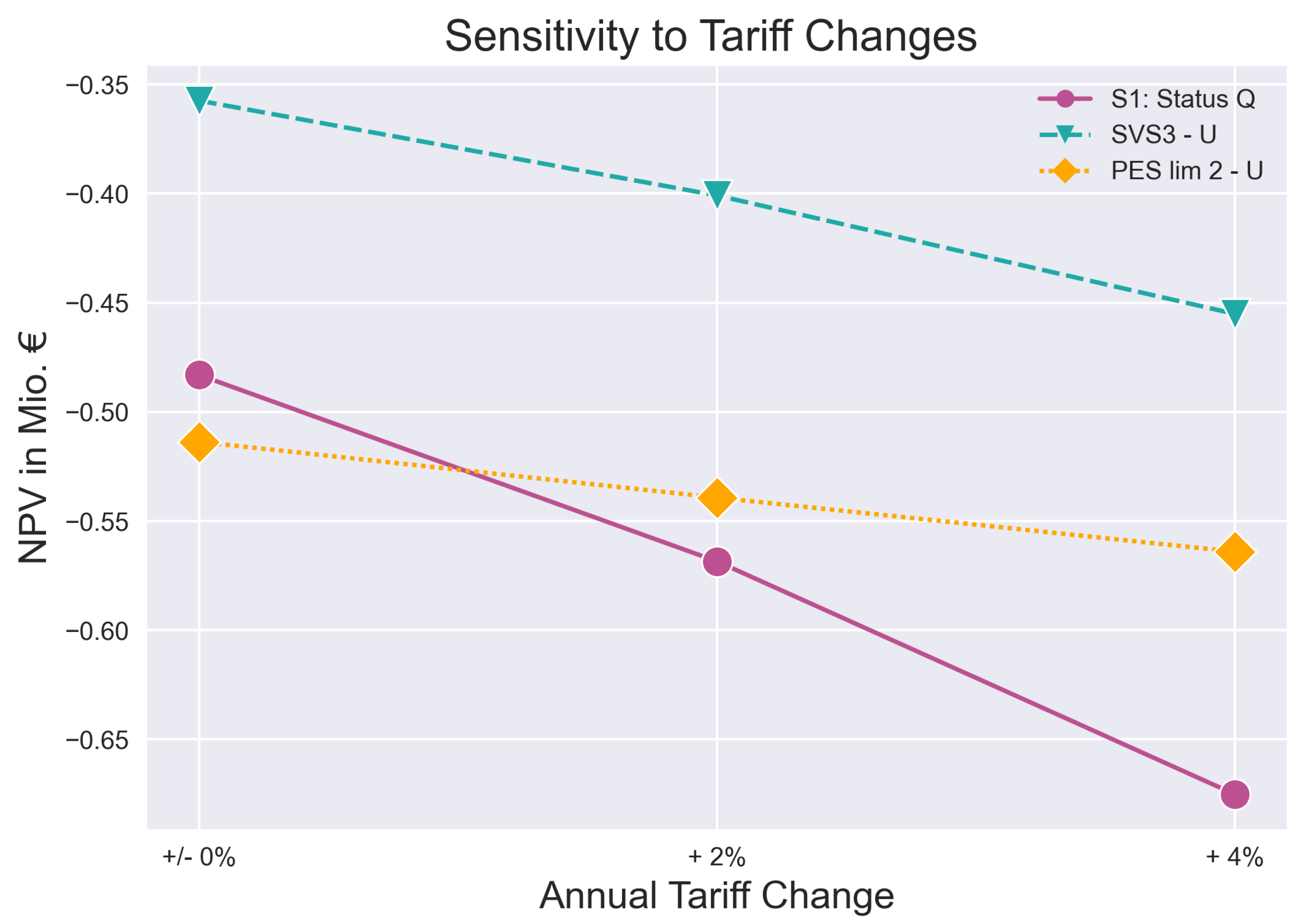
3.4. Variation of the Electricity Price

Figure 10 shows the sensitivity of the status quo scenario, the SVS3 scenario and the PES lim2–2 scenario towards an increase in the electricity tariff. Since the status quo scenario is only considering electricity import to cover the load, it is the most sensitive of the three towards an annual increase in electricity tariffs. Even with only the yearly 2% growth that resembles the average annual tariff increase in Europe, the status quo scenario has the lowest net present value over a lifetime. On the other hand, the grid power exchange limited scenario is the least affected by an increasing electricity price, given the used, dynamic tariff scheme. Being the only scenario among the three having a > 300 kWh battery installed, it can effectively reduce price peaks compared to the SVS3 scenario, which is dependent on the fluctuant behaviour of the sun.

4. Conclusions and Future Work

This work shows that Positive Energy Districts can be spatially feasible and economically superior over solely grid import in climatically favourable conditions, considering electricity demand only. This has been elaborated by applying a tailor-made linear programming model to an urban and rural case study with the same gross floor area on the island of La Palma. The rural area is more straightforward to convert to a PED due to its low floor space index. The much denser urban area with its higher FSI had to use some of the terrace space for PV power generation to achieve an annual positive energy balance. Thus, the FSI as an indicator for PED feasibility was confirmed, as already mentioned in [10]. However, due to the excellent climatic conditions, PV panels are sized until the limit of available space. While this favours the energy transition, it can be problematic for the grid, as amplitudes of power export fluctuations increase with higher PV installed capacity. This strains the grid, requires frequency regulations and potential expensive grid updates. A PED should contribute to neither of those, and thus, the grid export was restricted in this work to a multiple of the maximum demand. In most scenarios, this requires battery installations and PV power installed capacity is reduced. Furthermore, the model tries to distribute the azimuth angle of PV installations more evenly to spread the PV power generation over the day and therefore reduce expensive battery installations. Specifically, the battery addition reduces the net present value of a PED significantly. Only in some rural cases (more flexible PV installation distribution), the NPV stays above the one of status quo, as no/less battery is required compared to the urban scenarios.
The novel dynamic primary energy balancing mechanism appears promising for optimising PEDs or other collective energy systems, with some sort of energy storage for flexibility. The positive annual energy balance based on hourly changing PEFs of the grid mix provides an economic incentive to reduce primary energy consumption, which should be one of the central energy supply related goals of current times. This holds specifically for closed island (-like) systems such as the Canary Islands without their own electricity market. There, the price signals of the electricity tariff do not correspond to the local generation situation. Thus, it adds additional value over the static PEF approach proposed for PED evaluation by [11]. When applying such dynamic primary energy balancing, one critical point is allocating primary energy factors to specific export and import power streams, as this significantly affects the power exchange with the grid. This is further explained in Appendix A, where the grid to battery power flow PEF has been misallocated and resulted in undesirably battery charge and discharge behaviour.
Due to the dynamic PEF balance, the grid power exchange limited PED can be implemented less expensively in areas with high renewable grid mixes. Here, the battery capacity can be reduced as the significant differences in PEFs result in an excellent opportunity for PEF arbitrage. However, slight “cheating” could be identified particularly in the high RES scenario, where PV power is exported to the grid instead of covering the load as the model found it more valuable in terms of PEF at some time steps. This underlines the importance of correct adjustment of the PEF for each power flow. The low RES scenarios did not show this phenomenon to the same extent, as the PEF gap was too small to make up for the economic loss of this behaviour. Finally, a feasibility analysis towards increasing electricity tariffs revealed that the PED is more future proof towards raising electricity cost than the status quo scenario. Here, the grid exchange limited scenario, including a battery, is the most unaffected by the change, due to the added flexibility to react to price peaks. Thanks to the novel dynamic PEF approach, this work contributes to both, PED planning and operation approaches and is therefore a perfect addition to the aforementioned Annex 83 [16].
For future work, the primary energy led operation optimisation will be adjusted to not allow for “cheating” in any scenarios, such as covering the load demand by the grid while PV power is exported. A primary focus on self-consumption will be included. This would propose a valuable addition to microgrid/energy community operation in closed systems that do not have economic incentives for primary energy-saving operation due to a missing own electricity market. Additionally, the model will be extended to a mixed-integer linear programming model to account for heating and cooling in addition to electricity. To do so, a heating and cooling power matrix, similar to the electricity power matrix presented in this paper, will be introduced along with the mathematical description of each generation, conversion and storage technology. This will allow investigating less climatically favourable areas across Europe for their PED potential, including multi-energy demands. However, the introduction of binary variables and a much larger space of possible solutions will significantly increase the model-complexity. Finally, for reducing strain on the grid but still keeping up high renewable installation capacity, electric mobility addition to the modelling framework will be discussed in future research.

Author Contributions

Conceptualization, A.B., S.D.R. and H.A.; methodology, A.B.; software, A.B.; validation, A.B; formal analysis, A.B.; investigation, A.B.; resources, A.B. and S.D.R.; data curation, A.B.; writing—original draft preparation, A.B.; writing—review and editing, S.D.R., H.A. and A.B.; visualization, A.B.; supervision, S.D.R. and H.A.; project administration, S.D.R. and H.A. All authors have read and agreed to the published version of the manuscript.

Funding

This research has received funding from the European Union’s Horizon 2020 research and innovation programme under the Marie Skłodowska-Curie Actions, Innovative Training Networks, Grant Agreement No. 812730.

Institutional Review Board Statement

Not applicable.

Informed Consent Statement

Not applicable.

Data Availability Statement

Data used in this work is publicly available under: https://github.com/urbLexa/PEDSO_MDPI (accessed on 30 June 2021).

Acknowledgments

In addition to my supervisors Santiago Díaz Ruano and Hans Auer, I want to acknowledge Sebastian Zwickl-Bernhard, Lucía Dobarro Delgado and Salvador Suárez García for the support.

Conflicts of Interest

The authors declare no conflict of interest.

Abbreviations

The following abbreviations are used in this manuscript:
Δ Delta
CAPEXCapital Expenditure
C O 2 Carbon Dioxide
ECEuropean Commission
EPNEnergy Positive Neighbourhood
EUEuropean Union
exExport
FSIFloor Space Index
GFAGross Floor Area
GGSGrid Generation Mix Scenario
GTSGrid Tariff Scenario
imImport
KPIKey Performance Indicator
LPLinear Programming
MILPMixed Integer Linear Programming
NPVNet Present Value
PEDPositive Energy District
PEFPrimary Energy Factor
PESPower Exchange Scenario
PVPhotovoltaic
PVPCVoluntary Price for Small Consumer
REERed Eléctrica de España
tsTime step
RRural
SScenario
SETStrategic Energy Technology
SVSSpace Variation Scenario
UUrban
Units
°Degree
Euro
kWKilowatt
k W p Kilowatt peak
kWhKilowatt hour
m 2 Square meter
tTonnes

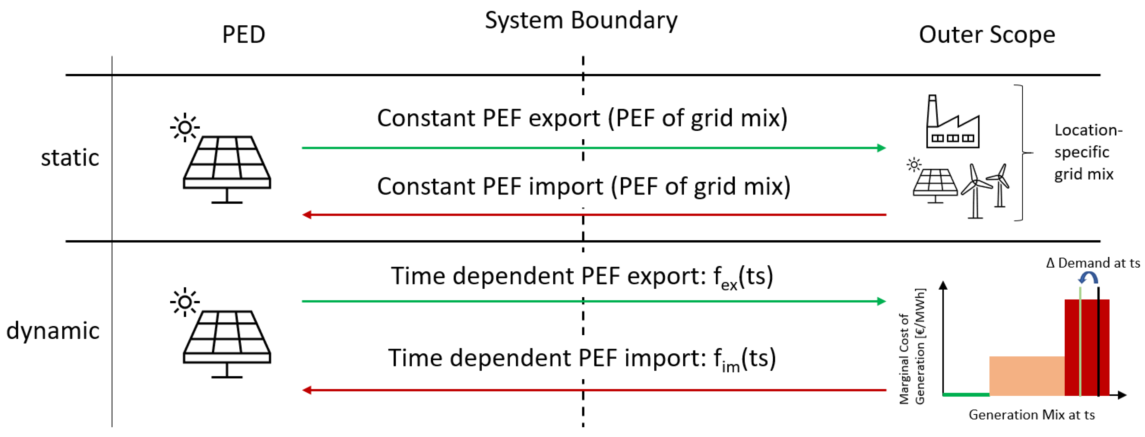
Appendix A. Primary Energy Factor of Import Electricity

Figure A1 shows the high importance of correct allocation of primary energy factors to power flows. In Figure A1, all import power was treated the same way in terms of PEF, no matter if it was used to cover the load that existed before PED creation or added new parts to the load by charging the battery. The PEF was the average over the grid mix PEFs at the current time step according to their share in the mix. For grid export, it was the PEF of the most expensive technology on the marginal cost curve at a current time step, as this one would be “substituted” by the PED’s electricity export. This would create the undesired behaviour of grid to battery power import contributing the negative average of the current grid mix PEF to the balance, while at the same time battery to grid export contributing with positively with the PEF of the marginally most expensive technology to the balance. This would leave a positive balance and therefore, reduce the need for battery installation in total, as the PED balance would be created partially by back and forth trading between battery and grid. Attributing also the PEF of the most expensive grid technology at a given time step to any electricity import that does not cover the load fixed ttheirror. However, it shows the importance of correct attribution of the PEF to corresponding power flows to not create undesired dispatch behaviour.
Figure A1. Battery charge and discharge power of PES lim2 scenario with wrong PEF for grid tp Battery power.
Energies 14 04864 g0a1

Appendix B. Input data

This section will supply the work with necessary information regarding input data. Table A1 shows data about the PV technology. PR stands for Performance Ration and takes into account typical additional losses of a PV system that are independent of the panel itself. GCR is the ground coverage ratio and takes into account spacing of PV panels to avoid shading. Data are obtained from [43].
Table A1. PV input data.
Input VariableValueUnit
CAPEX1070.0EUR/ k W p
OPEX fix12.8EUR/a
OPEX var0.0EUR/kWh
η p v 19%
PR0.84-
GCR flat0.8-
GCR tilt roof1-
Table A2 delivers the assumptions for lithium-ion battery technology. Assumptions are justified using [44,45,46]. Cap/Power ration defines the maximal charge and discharge power of the battery as a share of the available capacity. S O C 1 , 0 represents the initial state of charge at year 1 and hour 0.
Table A2. Battery input data.
Input VariableValueUnit
CAPEX750.0EUR/kWh
OPEX fix0.0EUR/a
OPEX var0.0EUR/kWh
η b a t t 95%
Cap/Power ratio0.3-
S O C 1 , 0 0kWh
Table A3 provides an overview about location specific data important for PV generation of the case study in Los Sauces, La Palma.
Table A3. Location input data.
Input VariableValueUnit
Latitude28.803-
Longitude−17.774-
Altitude288m
Albedo0.15-
Average Temperature17.8°C
Other important import data is shown in Table A4.
Table A4. Other input data.
Input VariableValueUnit
i0.05-
P E F d i e s e l 2.75-
C O 2 Emission factor diesel74.1t/TJ

References

  1. Rosales Carreón, J.; Worrell, E. Urban energy systems within the transition to sustainable development. A research agenda for urban metabolism. Resour. Conserv. Recycl. 2018, 132, 258–266. [Google Scholar] [CrossRef]
  2. IRENA. Rise of Renewables in Cities: Energy Solutions for the Urban Future; International Renewable Energy Agency: Abu Dhabi, United Arab Emirates, 2020; ISBN 978-92-9260-271-0. [Google Scholar]
  3. Groth, N.B.; Fertner, C.; Grosse, J. Urban energy generation and the role of cities. J. Settl. Spat. Plan. 2016, 5–17. [Google Scholar] [CrossRef]
  4. European Commission. SET-Plan ACTION n°3.2 Implementation Plan: Europe to Become a Global Role Model in Integrated, Innovative Solutions for the Planning, Deployment, and Replication of Positive Energy Districts. Available online: https://jpi-urbaneurope.eu/wp-content/uploads/2018/09/setplan_smartcities_implementationplan.pdf (accessed on 28 February 2020).
  5. European Commission. SETIS—SET Plan Information System. Available online: https://setis.ec.europa.eu/index_en (accessed on 3 June 2021).
  6. JPI Urban Europe / SET Plan Action 3.2. White Paper on PED Reference Framework for Positive Energy Districts and Neighbourhoods. Vienna. 2020. Available online: https://jpi-urbaneurope.eu/ped/ (accessed on 5 October 2020).
  7. Lindholm, O.; Rehman, H.U.; Reda, F. Positioning positive energy districts in European cities. Buildings 2021, 11, 19. [Google Scholar] [CrossRef]
  8. Cupelli, L.; Schumacher, M.; Monti, A.; Mueller, D.; De Tommasi, L.; Kouramas, K. Simulation Tools and Optimization Algorithms for Efficient Energy Management in Neighborhoods. In Energy Positive Neighborhoods and Smart Energy Districts; Academic Press: London, UK, 2017; pp. 57–100. [Google Scholar] [CrossRef]
  9. Schöfmann, P.; Zelger, T.; Bartlmä, N.; Schneider, S.; Leibold, J.; Bell, D. Zukunftsquartier—Weg zum Plus-Energie-Quartier in Wien; Federal Ministry for Climate Action, Environment, Energy, Mobility, Innovation and Technology: Vienna, Austria, 2020. [Google Scholar]
  10. Leibold, J.; Schneider, S.; Tabakovic, M.; Zelger, T.; Bell, D.; Schöfmann, P.; Bartlmä, N. ‘Zukunftsquartier’—On the Path to Plus Energy Neighbourhoods in Vienna. In Sustainability in Energy and Buildings: Proceedings of SEB 2019; Springer: Singapore, 2020; pp. 199–209. [Google Scholar] [CrossRef]
  11. Moreno, A.G.; Vélez, F.; Alpagut, B.; Hernández, P.; Montalvillo, C.S. How to achieve positive energy districts for sustainable cities: A proposed calculation methodology. Sustainability 2021, 13, 710. [Google Scholar] [CrossRef]
  12. Sougkakis, V.; Lymperopoulos, K.; Nikolopoulos, N.; Margaritis, N.; Giourka, P.; Angelakoglou, K. An Investigation on the Feasibility of Near-Zero and Positive Energy Communities in the Greek Context. Smart Cities 2020, 3, 19. [Google Scholar] [CrossRef]
  13. Ala-Juusela, M.; Crosbie, T.; Hukkalainen, M. Defining and operationalising the concept of an energy positive neighbourhood. Energy Convers. Manag. 2016, 125, 133–140. [Google Scholar] [CrossRef] [Green Version]
  14. ur Rehman, H.; Reda, F.; Paiho, S.; Hasan, A. Towards positive energy communities at high latitudes. Energy Convers. Manag. 2019, 196, 175–195. [Google Scholar] [CrossRef]
  15. Laitinen, A.; Lindholm, O.; Hasan, A.; Reda, F.; Hedman, Å. A techno-economic analysis of an optimal self-sufficient district. Energy Convers. Manag. 2021, 236. [Google Scholar] [CrossRef]
  16. IEA EBC. IEA EBC—Annex 83. Available online: https://annex83.iea-ebc.org/subtasks (accessed on 27 July 2021).
  17. Doubleday, K.; Parker, A.; Hafiz, F.; Irwin, B.; Hancock, S.; Pless, S.; Hodge, B.M. Toward a subhourly net zero energy district design through integrated building and distribution system modeling. J. Renew. Sustain. Energy 2019, 11. [Google Scholar] [CrossRef]
  18. Bakhtavar, E.; Prabatha, T.; Karunathilake, H.; Sadiq, R.; Hewage, K. Assessment of renewable energy-based strategies for net-zero energy communities: A planning model using multi-objective goal programming. J. Clean. Prod. 2020, 272. [Google Scholar] [CrossRef]
  19. Gremmelspacher, J.M.; Campamà Pizarro, R.; van Jaarsveld, M.; Davidsson, H.; Johansson, D. Historical building renovation and PV optimisation towards NetZEB in Sweden. Sol. Energy 2021, 223, 248–260. [Google Scholar] [CrossRef]
  20. Miftahurrahman, F.; Farizal; Dachyar, M. Optimization Model of Power Generation and Load Equipment Selection for near Zero Energy Building with Rooftop PV Integrated. In Proceedings of the 2019 6th IEEE International Conference on Engineering, Technologies and Applied Sciences (ICETAS 2019), Kuala Lumpur, Malaysia, 20–21 December 2019; Institute of Electrical and Electronics Engineers Inc.: New York, NY, USA, 2019. [Google Scholar] [CrossRef]
  21. Madathil, D.; Nair, M.G.; Jamasb, T.; Thakur, T. Consumer-focused solar-grid net zero energy buildings: A multi-objective weighted sum optimization and application for India. Sustain. Prod. Consum. 2021, 27, 2101–2111. [Google Scholar] [CrossRef]
  22. Lindberg, K.B.; Doorman, G.; Fischer, D.; Korpås, M.; Ånestad, A.; Sartori, I. Methodology for optimal energy system design of Zero Energy Buildings using mixed-integer linear programming. Energy and Buildings. Energy Build. 2016, 127, 194–205. [Google Scholar] [CrossRef] [Green Version]
  23. Zwickl-Bernhard, S.; Auer, H. Open-source modeling of a low-carbon urban neighborhood with high shares of local renewable generation. Appl. Energy 2021, 282. [Google Scholar] [CrossRef]
  24. Kriechbaum, L.; Scheiber, G.; Kienberger, T. Grid-based multi-energy systems-modelling, assessment, open source modelling frameworks and challenges. Energy Sustain. Soc. 2018, 8. [Google Scholar] [CrossRef] [Green Version]
  25. Groissböck, M. Are open source energy system optimization tools mature enough for serious use? Renew. Sustain. Energy Rev. 2019, 102, 234–248. [Google Scholar] [CrossRef]
  26. Openmod. Open Models. Available online: https://wiki.openmod-initiative.org/wiki/Open_Models (accessed on 30 June 2021).
  27. Bruck, A. PEDSO for MDPI Publication—Model and Data. 2021. Available online: https://github.com/urbLexa/PEDSO_MDPI (accessed on 30 June 2021).
  28. Wilkinson, M.D.; Dumontier, M.; Aalbersberg, I.J.; Appleton, G.; Axton, M.; Baak, A.; Blomberg, N.; Boiten, J.W.; da Silva Santos, L.B.; Bourne, P.E.; et al. Comment: The FAIR Guiding Principles for scientific data management and stewardship. Sci. Data 2016, 3. [Google Scholar] [CrossRef] [Green Version]
  29. European Commission. Energy Efficiency Targets. Available online: https://ec.europa.eu/energy/topics/energy-efficiency/targets-directive-and-rules/eu-targets-energy-efficiency_en (accessed on 30 July 2021).
  30. Hart, W.E.; Laird, C.; Watson, J.P.; Woodruff, D.L. Pyomo—Optimization Modeling in Python, 2nd ed.; Springer Nature: Cham, Switzerland, 2017; ISBN 978-1-4614-3225-8. [Google Scholar] [CrossRef]
  31. Hart, W.E.; Watson, J.P.; Woodruff, D.L. Pyomo: Modeling and solving mathematical programs in Python. Math. Program. Comput. 2011, 3, 219–260. [Google Scholar] [CrossRef]
  32. Esser, A.; Sensfuss, F. Evaluation of Primary Energy Factor Calculation Options for Electricity. 2016. Available online: https://ec.europa.eu/energy/sites/ener/files/documents/final_report_pef_eed.pdf (accessed on 11 May 2021).
  33. Eicker, U. Solare Technologien für Gebäude; Vieweg+Teubner Verlag: Wiesbaden, Germany, 2012; ISBN 978-3-8348-1281-0. [Google Scholar] [CrossRef]
  34. Holmgren, W.F.; Hansen, C.W.; Mikofski, M.A. pvlib python: A python package for modeling solar energy systems. J. Open Source Softw. 2018, 3, 884. [Google Scholar] [CrossRef] [Green Version]
  35. Gobierno de Canarias. Anuario EnergÉtico de Canarias 2019. 2020. Available online: https://www.gobiernodecanarias.org/cmsweb/export/sites/energia/doc/Publicaciones/AnuarioEnergeticoCanarias/20210219_AnuarioEnergeticoCanarias2019.pdf (accessed on 19 April 2021).
  36. La Palma Renovable. La Palma Renovable Promueve la primera Comunidad Energética Local de Canarias. Available online: https://lapalmarenovable.es/la-palma-renovable-promueve-la-primera-comunidad-energetica-local-de-canarias/ (accessed on 19 April 2021).
  37. Red Eléctrica de España. ESIOS Electricity · Data · Transparency. Available online: https://www.esios.ree.es/en (accessed on 20 April 2021).
  38. Minesterio para la Transición Ecológica. Real Decreto 244/2019, de 5 de abril, por el que se Regulan las Condiciones Administrativas, Técnicas y Económicas del Autoconsumo de Energía Eléctrica. 2019. Available online: https://www.boe.es/diario_boe/txt.php?id=BOE-A-2019-5089 (accessed on 20 April 2021).
  39. Red Eléctrica de España. Demanda Canaria en Tiempo Real. Available online: https://www.ree.es/es/actividades/sistema-electrico-canario/demanda-de-energia-en-tiempo-real (accessed on 20 April 2021).
  40. European Commission. TMY Generator|EU Science Hub. Available online: https://ec.europa.eu/jrc/en/PVGIS/tools/tmy (accessed on 20 April 2021).
  41. Eurostat. Electricity Price Statistics. Available online: https://ec.europa.eu/eurostat/statistics-explained/index.php?title=Electricity\_price\_statistics\#Electricity\_prices\_for\_household\_consumers (accessed on 20 May 2021).
  42. Red Eléctrica de España. Voluntary Price for the Small Consumer (PVPC). Available online: https://www.ree.es/en/activities/operation-of-the-electricity-systemvoluntary-price-small-consumer-pvpc (accessed on 1 July 2021).
  43. Danish Energy Agency. Technology Data—Generation of Electricity and District Heating. Available online: https://ens.dk/en/our-services/projections-and-models/technology-data/technology-data-generation-electricity-and (accessed on 12 April 2021).
  44. Danish Energy Agency. Technology Data–Energy Storage. Available online: https://ens.dk/en/our-services/projections-and-models/technology-data/technology-data-energy-storage (accessed on 12 April 2021).
  45. Fina, B.; Auer, H.; Friedl, W. Profitability of active retrofitting of multi-apartment buildings: Building-attached/integrated photovoltaics with special consideration of different heating systems. Energy Build. 2019, 190, 86–102. [Google Scholar] [CrossRef]
  46. Fina, B.; Auer, H.; Friedl, W. Profitability of PV sharing in energy communities: Use cases for different settlement patterns. Energy 2019, 189. [Google Scholar] [CrossRef]
Figure 1. PED Model Overview.
Energies 14 04864 g001
Figure 2. Static and dynamic electricity balance of a PED according to primary energy factors (PEF).
Energies 14 04864 g002
Figure 3. Location of case study: (a) Location of La Palma in the North-West of the Canarian Archipelago (red circle). (b) Location of Los Sauces in the North-East of La Palma (red circle). (c) Urban buildings considered for urban PED example (labelled in yellow). (d) Rural buildings considered for rural PED example (labelled in yellow).
Energies 14 04864 g003
Figure 4. (a) Tariff 2.0 DHA and feed-in tariff during 24th and 25th of August 2019. (b) Generation mix during 24th and 25th of August 2019.
Energies 14 04864 g004
Figure 5. Generation mix on the 24th and 25th August on the island of El Hierro.
Energies 14 04864 g005
Figure 6. Composition of the net present value by scenario in CAPEX, fixed costs, variable costs and revenue.
Energies 14 04864 g006
Figure 7. Density of grid import and export power without zeros over year one of SVS3—urban.
Energies 14 04864 g007
Figure 8. (a) NPV composition with power exchange limitations of the rural PED. (b) NPV composition with power exchange limitations of the urban PED. (c) Distribution of grid exchange power observations of PES lim2 rural. (d) Distribution of grid exchange power observations of PES lim2 urban.
Energies 14 04864 g008
Figure 9. Electricity dispatch on the 24th and 25th of August 2019 considering (a) load coverage under the low RES La Palma grid mix, (b) load coverage under the high RES El Hierro grid mix, (c) PV power distribution under the low RES La Palma grid mix, (d) PV power distribution under the high RES El Hierro grid mix, (e) Battery Charge and Discharge Power under the low RES La Palma grid mix and (f) Battery Charge and Discharge Power under the high RES El Hierro grid mix. Considered herein is the urban scenario with a grid exchange limit of 132 kW (PES lim2—U).
Energies 14 04864 g009
Figure 10. Sensitivity of the status quo (S1), the SVS3–U and the PES lim 2–U towards tariff increase.
Energies 14 04864 g010
Table 1. Model optimisation variables and parameters.
Model Decision Variables
c a p t e c Capacities of selected technologies
f u e l _ c o n s y , t s Fuel consumption at each time step each year (not used in this work)
p y , t s o u t , i n Power flow at each time step in each year depending on source (out) and target (in)
A a z , β Area used for PV installation for each angle pair
C y Annual costs
I 0 Investment cost at year 0
N P V Net Present Value - model objective
O _ M _ f i x y Annual fix costs
O _ M _ v a r y Annual variable costs
R y Annual Revenues
S O C y , t s State of charge of the battery at each time step each year
Other model parameters
η Efficiency
β Tilt angle
AArea
a z Azimuth angle
A Z Vector of considered azimuth angles
f e e d i n y , t s Feed-in Tariff at each ts
I r r Irradiance
P R Performance Ratio
G C R Ground Coverage Ratio
t a r i f f y , t s Tariff at each ts
t e c Specific technology
T E C Vector over all selected technologies
T I L T Vector of tilt angles
T S Number of time steps in one year
vOptimisation variable
VVector of optimisation variables
xTechnology with electricity output
XVector over technologies with electricity output
yYear
YTime horizon in years
zTechnology with electricity input
ZVector over technologies with electricity input
Table 2. Space available for PV generation on flat surfaces.
OccupationArea Urban [m2]Area Rural [m2]
Flat roof6783138
Terrace21502295
Water Storage02190
Total28288323
Table 3. Space available for PV generation on tilted roofs with tilt angle of 30°.
Azimuth Angle [°]Area Urban [m2]Area Rural [m2]
040235
450195
9029270
1350170
18040240
2250215
27090250
3150155
Table 4. Description of initial scenarios with the respective scenario number (S) and variation in available space for PV power generation with its respective space variation scenario number (SVS) for the rural (R) and urban (U) cases.
S #Description
1R & U: status quo
2R: no PED
3U: no PED
4R: PED
5U: PED
SVS #Description
1R: PED; no terrace or water storage for PV generation
2U: PED; no terrace for PV generation
3U/R: PED; 25% of terrace allowed if no PED possible in SVS 1/2
Table 5. NPV, optimised technology portfolio, electricity export/import ratio and C O 2 emissions of respective scenarios.
ScenarioNPV [€Mio]PV_flat
[kW p ]
PV_tilt roof
[kW p ]
Battery
[kWh]
Export/
Import
C O 2
Emissions [t]
S 1−0.483000-1971
S 2 & S 4−0.332126586012.60978
S 3 & S 5−0.3464301703.291047
SVS 1−0.3424778604.471025
SVS 2------
SVS 3—urban−0.3571852501.041134
Table 6. NPV, optimised technology portfolio, electricity export/import ratio and C O 2 emissions of respective PES.
ScenarioNPV [€Mio]PV_flat
[kW p ]
PV_tilt roof
[kW p ]
Battery
[kWh]
Export/
Import
C O 2
Emissions [t]
PES lim 2—R−0.3853818500.9421110
PES lim 1.5—R−0.445341921480.937944
PES lim 1—R−0.631292004240.928867
PES lim 2—U−0.514175293010.9321014
PES lim 1.5—U−0.698175295510.930976
PES lim 1—U−0.907176298420.926894
Table 7. NPV and optimised technology portfolio of S1&3 as well as all PE scenarios within a high RES penetrated grid mix.
ScenarioNPV [€Mio]PV_flat
[kW p ]
PV_tilt roof
[kW p ]
Battery
[kWh]
Export/
Import
C O 2
Emissions [t]
SVS1—R−0.3424778604.467476
PES lim 2—R−0.3707410800.727536
PES lim 1.5—R−0.39319172150.714567
PES lim 1—R−0.49381801780.671529
SVS3—U−0.3571852501.036530
PES lim 2—U−0.39215911610.696563
PES lim 1.5—U−0.495132291830.646586
PES lim 1—U−0.667130294070.626592
Publisher’s Note: MDPI stays neutral with regard to jurisdictional claims in published maps and institutional affiliations.

