Abstract
In modern systems, there is a tendency to model issues more accurately with low computational cost and considering multiscale decision-making which increases the complexity of the optimization. Therefore, it is necessary to develop tools to cope with these new challenges. Supply chain management of enterprise-wide operations usually involves three decision levels: strategic, tactical, and operational. These decision levels depend on each other involving different time scales. Accordingly, their integration usually leads to multiscale models that are computationally intractable. In this work, the aim is to develop novel clustering methods with multiple attributes to tackle the integrated problem. As a result, a clustering structure is proposed in the form of a mixed integer non-linear program (MINLP) later converted into a mixed integer linear program (MILP) for clustering shape-based time series data with multiple attributes through a multi-objective optimization approach (since different attributes have different scales or units) and minimize the computational complexity of multiscale decision problems. The results show that normal clustering is closer to the optimal case (full-scale model) compared with sequence clustering. Additionally, it provides improved solution quality due to flexibility in terms of sequence restrictions. The developed clustering algorithms can work with any two-dimensional datasets and simultaneous demand patterns. The most suitable applications of the clustering algorithms are long-term planning and integrated scheduling and planning problems. To show the performance of the proposed method, it is investigated on an energy hub as a case study, the results show a significant reduction in computational cost with accuracies ranging from 95.8% to 98.3%.
1. Introduction
1.1. Background and Motivation
Due to the multiscale dynamics in the solar system [1] multiscale phenomena are a significant part of human life. They have organized the time in terms of hours, days, months, and years. Although the main focus of interest is a system’s macroscale performance, the microscale is considered based on constitutive relations. On the other hand, while the focus is on the microscale, the compelling happens at a macroscale are not considered and the homogenous process at larger scale is assumed. However, this simple empirical approach cannot be extended to apply to more complex systems. Generally, the empirical approaches have a limited accomplishment for representing complicated or small scale systems in which the discrete or finite size effects are meaningful. In this regard, the multiscale modeling arises from the necessity to overcome the constraints of the aforementioned approaches (macro and microscale). Accordingly, multiscale simultaneously aims for the macroscale’s efficiency while maintaining the microscale’s models accuracy. The assessment of a problem from different levels and scales is a more comprehensive approach that represents a main change in modeling [1]. Integration across a supply chain’s decision level is crucial to improve returns on investment. Although planning and scheduling are interdependent both of them are usually carried out separately. The integration of planning and scheduling turns into improved decision level coordination and consequent operating costs reduction. However, the computational cost of the large scale problem is intractable because different time scales are integrated. Some methods have been proposed in the literature to overcome this issue. However, most of them have studied a specific problem or the proposed method is applicable to short time horizons. Clustering has a good potential to handle such problems by grouping similar input parameters together. This considerably shrinks the model size and improves computational tractability without compromising solution accuracy.
1.2. Literature Survey
Clustering has been widely utilized across different disciplines for more than 50 years. All clustering algorithms can be categorized into two groups: hierarchical and partitional. Likewise, big data analytics uses advanced analytic techniques to process very large and diverse datasets including: structured, semi-structured, and unstructured data; from different sources and sizes. Big data describes datasets sizing beyond the ability of conventional relational databases to capture, manage and process the data with low latency. Big data analysis allows taking better and quicker decisions using data that was previously considered computationally impossible due to sizing and structure state. Accordingly, businesses can use big data analytics to gain new insights from previously untapped databases. Mathematical programming plays a key role in clustering algorithm developments. For instance, Rao in [2] presented two integer programming formulations with different distance functions. The first formulation aims to minimize the sum of squares within groups, and leads to a mixed integer linear program (MILP) under certain conditions. The second formulation aims to minimize the maximum distance within groups, but leads to a mixed integer non-linear program (MINLP). Likewise, the authors in [3] formulated a MILP model for a company’s digital platform customer segmentation, as well as an improved algorithm to overcome computational complexity without compromising optimality. Furthermore, clustering also has applications to the power sector. Balachandra and Chandru in [4] grouped an entire year electricity demand into 9 clusters in sequence order using discriminant analysis. Then, the clusters were used as input for a resource constraint linear programming model of an electricity system based on supply demand matching in [5]. A fuzzy based clustering model in presented to model the uncertainty of electric vehicles load demand in [6,7], where, distributed generation is planned for a long-period horizon. In addition, several researchers have already investigated the two-scale scheduling-planning problem of energy systems. In [8], the authors have utilized a two stage metaheuristic algorithm for energy storage planning so that PSO algorithm is used for long-term planning and Tabu Search algorithm is used for short-term scheduling. A three loops optimization algorithm is proposed in [9] for optimal energy storage planning and scheduling, where new load demand of electric vehicles is also taken into account. However, in the mentioned works the metaheuristic algorithms have utilized for optimization that there is a significant concern about their results. A two-stage stochastic energy management approach is presented in [10] for a smart home scheduling, however, only short term operation is studied in this work and the long term planning is not considered. In a more recent study [11], the authors present two clustering algorithms formulated using integer programming with integral absolute error as similarity measure. The algorithms were effectively applied on electricity demand data clustering, as well as the unit commitment problem. However, the algorithm is limited to single-attribute data applications. Similarly, the authors in [12] developed a model to cluster electricity demand using k-means. The model was extended to include attributes such as heat demand, electricity price, and solar radiation. The clusters were used as input to optimize the energy systems’ operation to meet the urban district’s demand. The solution was compared to a reference value, but the study did not mention solution quality nor how it was solved.
1.3. Paper Contribution
The present work aims to tackle the integrated supply chain problem using a clustering approach. The aim is reducing model size by denoting the yearly days by typical days’ representative of the operating year. Although clustering has been widely employed in several applications, clustering of demand patterns has been poorly analyzed. Demand patterns in advanced energy systems are very complex given their multi-dimensional nature including shape (trajectory of the hourly demand curves), whereas time often displays diverse attributes (e.g., simultaneous demand for electricity and heat in advanced energy systems planning and scheduling in energy markets). Therefore, the flexibility of demand and supply should be modeled properly for energy transition. This study considers an extension of the previous work presented in [11], by incorporating the clustering of high-dimensional attributes instead of the traditional single attribute approach in order to plan and schedule the advanced energy systems. Accordingly, this study follows a mathematical programming-based approach and formulates the multi-dimensional attribute clustering algorithm using mixed integer programming techniques. Additionally, there is no indication on which algorithm type yields better results or the potential influence of sequence over solution quality. As a result, this work aims to investigate the aforementioned issues while providing a detailed analysis on the appropriate use of the novel clustering method for multiscale mathematical modeling. Proposed a MILP problem help us to achieve the global optimal solution for advanced energy systems planning and scheduling in energy markets. Additionally, to show the performance of the proposed method the clustering results are presented in two ways (normal and sequence clustering) and implemented on the electricity and heat demands. In order to demonstrate the application of the proposed method in the real world, this method is implemented for planning an energy hub as a case study.
2. The Proposed Clustering Algorithm
The present clustering algorithm is part of the time-series data; which has been gaining a lot of attention due to its potential applications to big data processing. The proposed algorithm can cluster demand data by simultaneously considering shape-similarity and trajectories-time. As a result, the clustered time-series data can assist easing the computational difficulty of multi-scale modeling. The L1-norm [13,14,15] (least absolute value method) was used to measure similarity and retain the model’s linearity and showcase the proposed algorithm generality.
The input parameters in process systems engineering usually consist of multiple attributes, such as the simultaneous demand of heat and electricity. Therefore, a clustering algorithm that simultaneously considers multiple attributes is proposed. The weighting method is chosen as multi-objective optimization approach [16] to deal with the multiple attributes nature of the problem. The typical model formulation for multi-objective optimization using the weighting method is given as follows:
where is the objective function for attribute a, is the weight factor for attribute a, , , and is the feasible region. and are the values for objective functions 1 and 2, respectively. The Pareto frontier is constructed by applying different combinations of weight factors. The utopia point () corresponds to the optimal values of objective functions 1 and 2 ( and ). However, the utopia point is usually infeasible. Therefore, the best solution is the closest to the utopia point.
2.1. General Algorithm Formulation
Given a set of load curves D (days) and H (hours) to be collected in C clusters, the aim is to assign days to clusters with the least dissimilarity. The following set of equations denotes a clustering model for minimizing the integral absolute error (IAE) or L1 norm for multiple attributes. The L1 norm has been widely used as a performance criterion in process control applications [17]. The formulation includes multiple attributes denoted by index while the application of the weighting method allows handling the multi-objective nature of the problem.
where IAEa is the integral absolute error used as a similarity measure for the a attribute. Equation (2) symbolizes the problem’s objective function as a weighted function between the performance criteria of the different attributes a under consideration, represents the weight factor for attribute a with the additional restriction that: , and . On the other hand, Equation (3) is the day assignment constraint requiring each day of the year to be assigned to a cluster of curves C. The binary variable denotes the assignment of load for the d-th day joining cluster c. The binary variable is equal to one if such an assignment takes place, and 0 otherwise. The IAE mathematical representation can be given as follows [18]:
where denotes the load curve(s) and the clustered curve(s). Equation (5) is a numerical evaluation of the norm L1 using the trapezoidal rule [19] for IAE between loads L and cluster curves C. Likewise, Equation (6) assesses the absolute difference between the load and cluster curves to be employed in the performance criterion.
where is the absolute difference between load curve L and clustered curve C for the hth hour in day d for attribute a, is the demand load of attribute a for the hth hour in day d, is the demand for the hth hour in cluster c and attribute a. The model construction is flexible in terms of performance criteria. As such, utilizing the L2 norm instead of the L1 norm is straightforward and requires the use of the Euclidean distance in Equation (4).
Moreover, the demand data can be sequentially clustered by including a set of constraints based on the string property concept [20]. Sequence clustering can be meaningful to maintain flexible operations. For example, in many occasions continuous similar operations are preferred to minimize the inconvenience and cost of change-overs and set ups. Accordingly, the following set of constraints (see Equations (7)–(9)) can be used to incorporate the time dimension into the clusters and require sequencing to be formed.
Equations (7)–(9) handle the first, intermediate, and last clusters sequence, respectively. Moreover, the next equation is equivalent to the previous set of constraints provided that the non-existing terms are dropped out the mathematical expression. This feature is built-in in many algebraic modeling systems such as GAMS.
The above formulation provides a unique platform for performing normal and sequence clustering since it is based on an equivalent algorithmic structure. Nonetheless, the formulation renders a MINLP model due to the absolute value and multiplication between the variables and shown in Equation (6). Accordingly, the absolute function can be linearized employing the following mathematical expressions [21]:
Once the load curve is chosen (), one of the constraints takes on a negative value while the remaining is positive. As a result, the constraint with a negative right-hand side becomes redundant; whereas equals the positive difference [22]. Even though the aforementioned approach eliminates the absolute value in the model, the bilinear term () persists. This term can be further linearized introducing a new continuous variable through the following set of constraints [23]:
where is the employed relaxation variable for the linearization method, and are the lower and upper bound of attribute a load for the hth hour, respectively. Applying the aforementioned linearization approach renders the model to be an MILP; and, therefore, more computationally tractable.
Equation (19) is only required for the sequence clustering case. The above model is a mathematical representation of clustering trajectories of time series data of different attributes and aims to achieve clusters through the L1 norm minimization.
2.2. Size-Reduction Heuristic Algorithm for Multiple Attributes
Since the computational complexity of the aforementioned clustering model is evident, a heuristic algorithm is proposed to handle the issue, including its multiple attributes nature. The algorithm is based on an iterative structure which compares lower and upper bound solutions. This type of structure has been employed in the past and represents an appropriate solution procedure to tackle large-scale mathematical models [3,24]. This subsection aims to extend the applicability of the previously proposed MILP model to long planning horizons. Nonetheless, the proposed modeling framework keeps its linearity and programming basis. The heuristic follows the k-means algorithm; but this time the clusters are built using the mathematical models previously proposed. The k-means is typically applied to one-dimensional time-series data, but there are versions able to deal with trajectories. The k-means algorithm is given as follows: (1) randomly initialize k partitions, (2) calculate a cluster prototype matrix M, (3) allocate each item in the dataset to the nearest cluster, (4) recalculate cluster prototype matrix M based on present partition, and (5) repeat procedure until no change is noticed in the estimated clusters.
Figure 1 shows the flowchart of the proposed heuristic algorithm for multiple attributes. The heuristic is executed for each weight factor combination. The procedure is given as follows: (1) n random clusters or scenarios are generated. The scenarios can be generated in Microsoft Excel® by randomizing between maximum and minimum of each hour for each attribute in the entire demand curves. (2) Each weight factor is considered starting with the first scenario. At the first try, the clusters are fixed in the MILP model, and the resulting integer program is solved for day assignment providing an upper bound on the solution. (3) The day assignment is fixed and the linear programming model is solved to reach a lower bound on the solution. The solution is considered as the current best if the variance between the upper and lower bounds is within the acceptable pre-specified period. In this situation, the next scenario is considered. Otherwise, for a given scenario, the process is reaped between fixing clusters and day assignment until the upper and lower bounds difference fall within the acceptable tolerance. (4) Once all scenarios are considered for a given weight factor, the process goes to the next weight factor and the steps repeated until all weight factors have been considered. The proposed model can be applied for both normal and sequence clustering. The common formulation can be employed in the both types of clustering for problems with multiple attributes. The mathematical models were built in the General Algebraic Modeling System (GAMS).
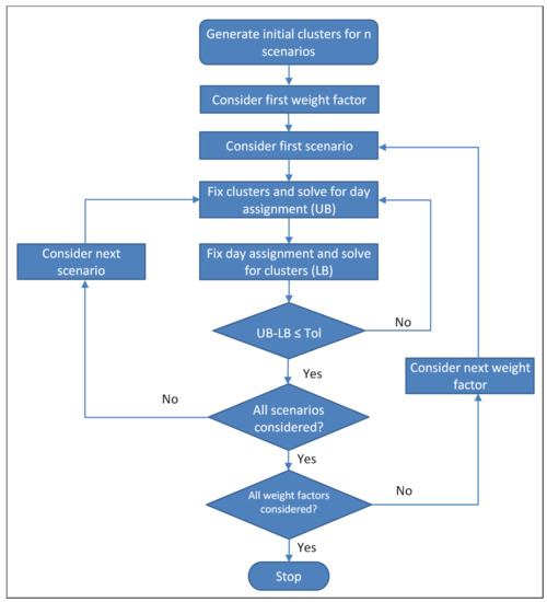
Figure 1.
Flowchart of proposed heuristics algorithm for multiple attributes.
3. Model Verification and Numerical Results
3.1. Proposed Model Verification and Assessment
In this section, the computational performance and outputs of the multiple attribute clustering algorithm are presented. Random values between the maximum and minimum of each hour are generated in Excel. Nonetheless, there is a slight difference for generating the sequence clustering’s initial guess. For instance, the days are initially partitioned based on days to clusters ratio (the ratio must be rounded down). Accordingly, if we have 30 days and 3 clusters the ratio is 10; thus, resulting in 3 partitioned days’ groups. Afterward, cluster 1’s initial guess is generated by randomizing between each hour’s maximum and minimum in the first partitioned days. Similarly, this approach is applied to clusters 2 and 3. The aforementioned procedure yields improved objective function values; while the ratio itself could be optimized by carefully analyzing the demand. The runs for this case study include 4, 5, and 6 clusters for an entire year (365 days) for normal and sequence clustering, respectively (i.e., 6 runs in total). Moreover, 25 scenarios were generated per run. The GAMS/CPLEX solver was used to perform the runs on an Intel (R) Xeon (R) 2.4 GHz (2 processors), 16 GB RAM workstation. It is worth mentioning that parameter tuning was used for sequence clustering to reduce solution time. The algorithm tolerance was set to 10–4. In this case, study, an energy hub system’s hourly heat and electricity demands during a year is used for illustration purposes that is presented in [25], where, the heat and electricity demands are extracted. Table 1 shows the 8 weight factor combinations used to determine the Pareto frontier. The priority between heat and electricity varies among the weight factor combinations. For example, weight factor 1 leans towards heat while weight factor 8 leans toward electricity (see Table 1 for details).

Table 1.
Multi-objective function weight factors.
Table 2 lists the solution time for the case study runs. The solution time for sequence clustering is shorter than normal clustering even for equivalent order of magnitude. The extra constraint sets in sequence clustering reduce the feasible region size; thus, resulting in shorter solution times. As can be noticed, increasing the model size by rising the number of clusters has a negative impact on solution time. The model is hard to solve even with a small number of binary variables.
Table 2.
Case study runs’ solution times.
The Pareto frontiers for normal and sequence clustering are shown in Figure 2 and Figure 3, respectively. As presented in Table 1, the Pareto frontiers are captured for all runs with the weight factor combinations. As shown in the figures an improved objective function value is achieved when the number of clusters increases for both: normal and sequence clustering.
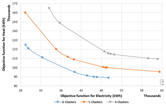
Figure 2.
Pareto frontiers for normal clustering.
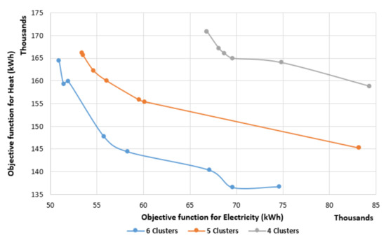
Figure 3.
Pareto frontiers for sequence clustering.
Table 3 and Table 4 show the results of 5 clusters for normal and sequence clustering, respectively. With the intention to gain results’ insight, a relative error function is employed as validation measure between the cluster and curve loads as follows:
where is the relative error between the cluster and curve loads. Fundamentally, this metric is the L1 criterion scaled by the load curve to enable comparisons when the demand curves greatly differ in magnitude. As a result, the error measurement can be effectively employed to assess performance given its independence from the system capacity and measurement unit. This error measurement criteria is the most widely used method in utility forecasting; although high error values can be anomalies instead of simple incorrect predictions [26]. Accordingly, the error standard deviation of curves in the same cluster is adopted to check that curves within the same clusters have high similarity; while curves in different clusters have low similarity. Additionally, graphical and visual comparisons are used to assess similarity.
Table 3.
Computational statistical errors for normal clustering 365 days-5 clusters (365-5).
Table 4.
Computational statistical errors for sequence clustering 365 days-5 clusters (365-5).
With comparison of the objective function value, error average, and standard deviation, it can be found the normal clustering had better results than sequence clustering. This is due to extra sequence requirement in sequence clustering executes that might be needed in certain process operations to minimize set-ups. As it can be noticed from Table 3 and Table 4, there is a results changeover as weight factors vary. Moreover, it was found that heat demand contains zero value elements in certain periods. For these particular instances, the relative error calculation is not performed to avoid division by zero. Accordingly, relative error calculations were troublesome for demands close to zero. However, the heat demand’s error average and standard deviation are amplified. This latter results from the significant fluctuation in heat demand. Although the demand ranges from 0 to 250 kW, the relative error calculation is still difficult. For example, if the demand is 0.1 kW and cluster value 1 kW; the relative error turns into 900%. Furthermore, the electricity demand’s error average and standard deviation are relatively small compared to the heat. The weight factor has an important impact on clusters. For example, with increasing the clusters number, its quality will be enhanced. In comparison with the sequence cluster, the normal cluster has more flexibility. In the procedure of electricity demand clustering, especially in sequence, many clusters overlap each other. However, these clusters cannot be merged as they correspond for different days and the heat demand for these days are different. Therefore, for any application that do not require sequencing it is suggested to use normal clustering to minimize the computational cost especially in large scale case studies.
3.2. Case Study: Application of Multiple Attribute Clustering to Energy Hubs
This case study shows an application of the proposed clustering algorithms to utility demand data involving multiple attributes; as well as investigating its impact on solution accuracy. It has already been established in the previous section that clustering significantly reduces the computational burden. More specifically, this case study assesses the outputs of the proposed normal and sequence clustering algorithms against a full energy hub model with multiple demand attributes that does not employ clustering. In the energy hub problem, the operation cost should be minimized as a medium term decision level problem. Planning of an energy hub is considered as a case study, because energy hubs are known as a promising tool to increase the efficiency of the system. Additionally, the accuracy of the clustering results for heat and electricity demands are so important in energy hubs, since the day-ahead operation and generation expansion planning of them is done based on the load demands curves, and results with low accuracy led to a big penalty cost for energy hub operators. The energy hubs can be modeled based on heuristic algorithms or mathematical programming. In this study, it is modeled as a linear programming (LP) mode [25] as presented below.
3.2.1. Energy Hub Model Formulation
The objective of the work is to minimize the operation cost of the studied energy hub system, while the operating areas constraint of the units are taken into account. Figure 4 shows the energy hub schematic. It consists of one boiler, one combined heat and power (CHP) unit, and the option to purchase electricity from the grid. The boiler and CHP are supplied by natural gas. As mentioned before, the electricity demand is supplied by upstream grid and the CHP unit and the heat demand is supplied by the boiler and CHP unit [27].
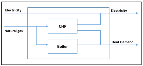
Figure 4.
Schematic for the energy hub system.
Equation (21) denotes the energy hub’s objective (cost) function. It is essentially the energy hub’s operating cost, which includes: fuel (gas) consumption, operation and maintenance, and grid expenses. This is given as follows:
where CF ($/h) is the cost objective function, (kW) is the CHP’s electricity generation at the hth hour of the dth day, (kW) is the CHP’s heat generation at the hth hour of the dth day, ($/kWh) is the CHP’s operation and maintenance cost, (kW) is the boiler’s heat generation at the hth hour of the dth day, ($/kWh) is the boiler’s operation and maintenance cost, (m3/h) is the CHP’s natural gas consumption at the hth hour of the dth day, (m3/h) is the boiler’s natural gas consumption at the hth hour of the dth day, ($/m3) is the natural gas price, (kW) is the electricity consumed from the grid at the hth hour of the dth day, and ($/kWh) is the grid’s hourly electricity price.
The electricity and heat demands are satisfied at any hth hour of day d as shown in Equations (22) and (23), respectively.
where (kW) and (kW) are the hourly electricity and heat demands, respectively.
Furthermore, Equations (24) and (25) ensure that the power produced by the CHP and heat by the boiler at any time are within their corresponding generation capacities as follows [27]:
where (kW) and (kW) are the maximum installed power and heat generation capacities for the CHP unit and boiler, respectively.
The following set of Equations (26)–(28) allows calculating the amount of utilities produced by the energy hub:
where is the CHP’s electrical efficiency, the CHP’s thermal efficiency, the boiler’s thermal efficiency, and b is a unit conversion factor for the natural gas flowrate. All model’s parameter values are given in Table 5.
Table 5.
Energy hub model parameters.
3.2.2. Simulation Results and Discussions
The electricity and heat demands, as well as a number of clusters from Section 3, are used as inputs for the present energy hub model. For comparison purposes, the objective cost function is multiplied by a parameter named (as illustrated in Equation (29)) that let us to compare the full scale model and clustered cases. The repetitions number is represented by parameter for corresponding d day. This parameter is equal to 1 for full scale case and is equal to days’ number for the clustered cases. For instance, of cluster 1 will be equal to 40 if cluster 1 represents 40 days.
The full scale model considers hourly heat and electricity demands loads for 365 days; whereas the clustered cases hourly loads take into account 4, 5, and 6 clusters (clusters are considered as days). Since the energy hub model is a LP, it just takes a few seconds to solve the full scale case, which made it difficult to illustrate the advantages of clustering applications in terms of solution time reduction at least for this particular example. However, the reduction in computational time through the use of clustering has been established in the previous section. In this section, the focus instead is solution quality.
The values of the objective function for the full scale case is presented in Table 6. For a better assessment, the objective function values are plotted along with the relative error and are compared with the optimal case as shown in Figure 5. As can be seen, considering the objective function value all clustered cases are underestimated. In comparison with the sequence clustering, the normal clustering is closer to the optimal case. The average error of the objective function is −1.7% and −4.2% for normal and sequence clustering, respectively. In addition, with increasing the number of clusters, the solution quality will be enhanced for both normal and sequence clustering. Moreover, the weight factor variation does not have a significant effect on the objective function values. This is due to the high correlation between heat and electricity demands.
Table 6.
Energy hub model’s objective function values (thousand USD) for full scale case.
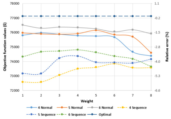
Figure 5.
Energy hub’s objective function values for all runs and weight factors.
In order to examine the effect of increasing the number of clusters, Figure 6 and Figure 7 showcase the energy hub utility production rates for the normal and sequence clustering cases for weight factors 1 and 8, respectively. Increasing the number of clusters improves the solution quality as it closes the gap between the optimal non-clustered and clustered case. In addition, the results of weight factor 1 are much closer to the optimal non-clustered case because it leans towards the heat demand. As the heat demand shows the higher variability among utilities, prioritizing the heat demand allows keeping it the closest to the original value; thus, minimizing the errors caused by the clusters variability. Moreover, as one could expect normal clustering showcases higher solution quality than sequence clustering due to the constraints require for sequencing.
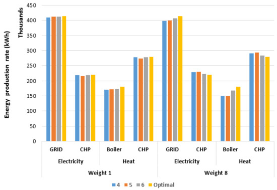
Figure 6.
Energy hub’s utility production rates for normal clustering with weight factors 1 and 8.
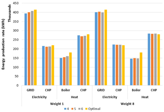
Figure 7.
Energy hub’s utility production rates for sequence clustering with weight factors 1 and 8.
In order to examine the weight factors effect, Figure 8 and Figure 9 illustrate the energy hub’s utilities production rates for all weight factors for normal and sequence clustering with 5-clusters, respectively. As shown in the figures, varying the weight factors has a gradual effect on solution quality as the priority switches from heat to electricity. Nonetheless, varying the weight factors does not have a drastic effect on the objective function values. This might be due to the fact that the electricity and heat demands have equivalent symmetry over the whole horizon. Additionally, as previously stated the weight factor 1 results are much closer to the optimal non-clustered case.
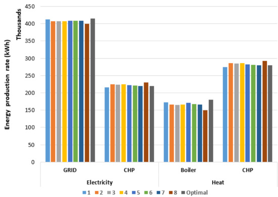
Figure 8.
Energy hub’s utility production rates for all weight factors in normal clustering with 5-clusters case.
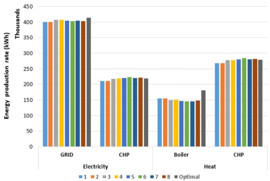
Figure 9.
Energy hub’s utility production rates for all weight factors in sequence clustering with 5-clusters case.
4. Conclusions
In this paper, a mathematical programming approach for multiscale models with multiple attributes that are computationally intractable was proposed. The advantages of the proposed method are simplicity to implement it with low computational cost, also the proposed method is a mixed-integer linear programming which can guarantee obtain the global optimal solution. To show the performance of the proposed method the clustering results are presented in two ways (normal and sequence clustering) and implemented on the electricity and heat demand because demand patterns are very complex given their multi-dimensional nature. The results show that a better objective function is achieved when the number of clusters increases for both normal and sequence clustering as it closes the gap between the optimal (full-scale model) and clustered cases’ solutions. Normal clustering results are found to be better than sequence clustering in terms of objective function value, error average, and standard deviation. The statistical analysis of the heat demand was challenging as suggested by the results. This is due to the huge fluctuation in the heat demand; particularly, for demands close to zero. The flexibility of normal clustering has a major advantage over sequence. There are many clusters of electricity demand, especially sequence clusters, overlapping with each other. They cannot be merged since they correspond to different days and heat demand clusters for these days are different. Therefore, for applications that do not require sequencing, it is advantageous to use normal clustering to minimize computational effort and deal with large-scale models. Additionally, in order to demonstrate the application of the proposed method in the real world, this method is implemented for planning an energy hub as a case study. The results show that all clustered cases are underestimated in terms of objective function value. Normal clustering is closer to the optimal compared with sequence. The objective function error average is −1.7% for normal clustering while for sequence clustering is −4.2%. Moreover, varying the weight factors does not have a significant effect on the objective function value. This might be due to a similar symmetry in the heat and electricity demands. In addition, the weight factor 1’s results (prioritizing heat demand) are much closer to the optimal case.
Author Contributions
Conceptualization, F.A., A.A. and A.E.; methodology, F.A., A.A. and A.E.; software, F.A.; validation, F.A., A.A. and A.E.; formal analysis, F.A., A.A. and A.E.; investigation, F.A., A.A. and A.E.; resources, F.A.; data curation, F.A.; writing—original draft preparation, F.A.; writing—review and editing, A.A. and A.E.; visualization, F.A.; supervision, A.A.; project administration, A.E.; funding acquisition, A.E. All authors have read and agreed to the published version of the manuscript.
Funding
This research received no external funding.
Conflicts of Interest
The authors declare no conflict of interest.
Nomenclature/Abbreviations
| MILP | Mixed integer linear programming |
| MINLP | Mixed integer nonlinear programming |
| Std | Standard |
| Avg | Average |
| CHP | Combined heat and power |
| GAMS | General algebraic modeling system |
| LP | Linear programming |
Variables
| Absolute difference between load curve L and clustered curve C for the hth hour in day d for attribute a | |
| b | Unit conversion factor for the natural gas flowrate |
| Lower bound of attribute a load for the hth hour | |
| Upper bound of attribute a load for the hth hour | |
| C | Clusters |
| Cost objective function | |
| D | Load curves |
| Demand for the hth hour in cluster c and attribute a | |
| Demand load of attribute a for the hth hour in day d | |
| CHP’s electricity generation at the hth hour of the dth day | |
| Electricity consumed from the grid at the hth hour of the dth day | |
| Relative error between the cluster and curve loads | |
| Objective function for attribute a | |
| H | Hours |
| Boiler’s heat generation at the hth hour of the dth day | |
| CHP’s heat generation at the hth hour of the dth day | |
| IAEa | Integral absolute error used as a similarity measure for the a attribute |
| Hourly electricity demand in the dth day | |
| Hourly heat demand in the dth day | |
| M | Matrix |
| Maximum installed power and heat generation capacities for the CHP unit | |
| Maximum installed heat generation capacity for the boiler | |
| Number of repetitions (frequency) for corresponding d day | |
| Boiler’s natural gas consumption at the hth hour of the dth day | |
| CHP’s natural gas consumption at the hth hour of the dth day | |
| Boiler’s operation and maintenance cost | |
| CHP’s operation and maintenance cost | |
| Natural gas price | |
| Grid’s hourly electricity price | |
| Relaxation variable for the linearization method | |
| Feasible region | |
| Weight factor for attribute a | |
| Binary variable denoting the assignment of load for the dth day joining cluster c |
Greek Symbols
| Value for objective function 1 | |
| Value for objective function 2 | |
| Utopia point | |
| CHP’s electrical efficiency | |
| CHP’s thermal efficiency | |
| Boiler’s thermal efficiency |
Subscripts
| a | Type of attribute |
| c | Cluster |
| d | Day |
| h | Hour |
Superscript
| elec | Electricity |
| NG | Natural gas |
References
- Weinan, E. Principles of Multiscale Modeling; Cambridge University Press: Cambridge, UK, 2011. [Google Scholar]
- Rao, M.R. Cluster analysis and mathematical programming. J. Am. Stat. Assoc. 1971, 66, 622–626. [Google Scholar] [CrossRef]
- Sağlam, B.; Salman, F.S.; Sayın, S.; Türkay, M. A mixed-integer programming approach to the clustering problem with an application in customer segmentation. Eur. J. Oper. Res. 2006, 173, 866–879. [Google Scholar] [CrossRef]
- Balachandra, P.; Chandru, V. Modelling electricity demand with representative load curves. Energy 1999, 24, 219–230. [Google Scholar] [CrossRef]
- Balachandra, P.; Chandru, V. Supply demand matching in resource constrained electricity systems. Energy Convers. Manag. 2003, 44, 411–437. [Google Scholar] [CrossRef]
- Ahmadian, A.; Sedghi, M.; Aliakbar-Golkar, M. Fuzzy load modeling of plug-in electric vehicles for optimal storage and DG planning in active distribution network. IEEE Trans. Veh. Technol. 2016, 66, 3622–3631. [Google Scholar] [CrossRef]
- Ahmadian, A.; Sedghi, M.; Elkamel, A.; Aliakbar-Golkar, M.; Fowler, M. Optimal WDG planning in active distribution networks based on possibilistic–probabilistic PEVs load modelling. IET Gener. Transm. Distrib. 2017, 11, 865–875. [Google Scholar] [CrossRef]
- Sedghi, M.; Ahmadian, A.; Aliakbar-Golkar, M. Optimal storage planning in active distribution network considering uncertainty of wind power distributed generation. IEEE Trans. Power Syst. 2015, 31, 304–316. [Google Scholar] [CrossRef]
- Ahmadian, A.; Sedghi, M.; Aliakbar-Golkar, M.; Elkamel, A.; Fowler, M. Optimal probabilistic based storage planning in tap-changer equipped distribution network including PEVs, capacitor banks and WDGs: A case study for Iran. Energy 2016, 112, 984–997. [Google Scholar] [CrossRef]
- Zeynali, S.; Rostami, N.; Ahmadian, A.; Elkamel, A. Two-stage stochastic home energy management strategy considering electric vehicle and battery energy storage system: An ANN-based scenario generation methodology. Sustain. Energy Technol. Assess. 2020, 39, 100722. [Google Scholar] [CrossRef]
- Alhameli, F.; Elkamel, A.; Betancourt-Torcat, A.; Almansoori, A. A mixed-integer programming approach for clustering demand data for multiscale mathematical programming applications. AIChE J. 2019, 65, e16578. [Google Scholar] [CrossRef]
- Fazlollahi, S.; Becker, G.; Maréchal, F. Multi-objectives, multi-period optimization of district energy systems: III. Distribution networks. Comput. Chem. Eng. 2014, 66, 82–97. [Google Scholar] [CrossRef] [Green Version]
- Bekta, S. The comparison of L11 and L22-norm minimization methods. Int. J. Phys. Sci. 2010, 5, 1721–1727. [Google Scholar]
- Chelmis, C.; Kolte, J.; Prasanna, V.K. Big data analytics for demand response: Clustering over space and time. In Proceedings of the 2015 IEEE International Conference on Big Data (Big Data), Santa Clara, CA, USA, 29 October–1 November 2015; IEEE: Piscataway, NJ, USA, 2015; pp. 2223–2232. [Google Scholar]
- Green, R.; Staffell, I.; Vasilakos, N. Divide and Conquer? k-Means Clustering of Demand Data Allows Rapid and Accurate Simulations of the British Electricity System. IEEE Trans. Eng. Manag. 2014, 61, 251–260. [Google Scholar] [CrossRef]
- Branke, J.; Branke, J.; Deb, K.; Miettinen, K.; Slowiński, R. Multiobjective Optimization: Interactive and Evolutionary Approaches; Springer Science & Business Media: Berlin/Heidelberg, Germany, 2008; p. 5252. [Google Scholar]
- Singh, S.K. Process Control: Concepts Dynamics and Applications; PHI Learning Pvt. Ltd.: New Delhi, India, 2009. [Google Scholar]
- Nagode, K.; Škrjanc, I. Modelling and internal fuzzy model power control of a Francis water turbine. Energies 2014, 7, 874–889. [Google Scholar] [CrossRef] [Green Version]
- Yin, B.; Liu, Y.; Li, H.; Zhang, Z. Efficient shifted fractional trapezoidal rule for subdiffusion problems with nonsmooth solutions on uniform meshes. BIT Numer. Math. 2021, 1–36. [Google Scholar] [CrossRef]
- Vinod, H.D. Integer programming and the theory of grouping. J. Am. Stat. Assoc. 1969, 64, 506–519. [Google Scholar] [CrossRef]
- Mangasarian, O.L. Absolute value equation solution via dual complementarity. Optim. Lett. 2013, 7, 625–630. [Google Scholar] [CrossRef] [Green Version]
- Gougheri, S.S.; Jahangir, H.; Golkar, M.A.; Moshari, A. Unit commitment with price demand response based on game theory approach. In Proceedings of the 2019 International Power System Conference (PSC), Tehran, Iran, 9–11 December 2019; IEEE: Piscataway, NJ, USA, 2019; pp. 234–240. [Google Scholar]
- Sirikitputtisak, T.; Mirzaesmaeeli, H.; Douglas, P.L.; Croiset, E.; Elkamel, A.; Gupta, M. A multi-period optimization model for energy planning with CO2 emission considerations. Energy Procedia 2009, 1, 4339–4346. [Google Scholar] [CrossRef] [Green Version]
- Üney, F.; Türkay, M. A mixed-integer programming approach to multi-class data classification problem. Eur. J. Oper. Res. 2006, 173, 910–920. [Google Scholar] [CrossRef]
- Maroufmashat, A.; Elkamel, A.; Fowler, M.; Sattari, S.; Roshandel, R.; Hajimiragha, A.; Walker, S.; Entchev, E. Modeling and optimization of a network of energy hubs to improve economic and emission considerations. Energy 2015, 93, 2546–2558. [Google Scholar] [CrossRef]
- Bakker, M.; Van Duist, H.; Van Schagen, K.; Vreeburg, J.; Rietveld, L. Improving the performance of water demand forecasting models by using weather input. Procedia Eng. 2014, 70, 93–102. [Google Scholar] [CrossRef] [Green Version]
- Gougheri, S.S.; Jahangir, H.; Golkar, M.A.; Ahmadian, A.; Golkar, M.A. Optimal participation of a virtual power plant in electricity market considering renewable energy: A deep learning-based approach. Sustain. Energy Grids Netw. 2021, 26, 100448. [Google Scholar] [CrossRef]


Publisher’s Note: MDPI stays neutral with regard to jurisdictional claims in published maps and institutional affiliations. |
© 2021 by the authors. Licensee MDPI, Basel, Switzerland. This article is an open access article distributed under the terms and conditions of the Creative Commons Attribution (CC BY) license (https://creativecommons.org/licenses/by/4.0/).