Abstract
The implementation of district heating networks into cities is a main topic in policy planning that looks for sustainable solutions to reduce CO2 emissions. However, their development into cities is generally limited by a high initial investment cost. The development of optimization methods intended to draft efficient systems using heating consumption profiles into a prescribed geographic area are useful in this purpose. Such tools are already referred to in the scientific literature, yet they are often restricted to limit the computational load. To bridge this gap, the present contribution proposes a multi-period mixed integer linear programming model for the optimal outline and sizing of a district heating network maximizing the net cash flow based on a geographic information system. This methodology targets a large range of problem sizes from small-scale to large-scale heating networks while guaranteeing numerical robustness. For sake of simplicity, the developed model is first applied to a scaled down case study with 3 available heating sources and a neighborhood of 16 streets. The full-scale model is presented afterwards to demonstrate the applicability of the tool for city-scale heating networks with around 2000 streets to potentially connect within a reasonable computational time of around only one hour.
1. Introduction
In the context of current environmental problems, issues related to the energy transition are of paramount importance for the upcoming years. The question of energy policy to meet these challenges concerns all parts of the population: political decision-makers, industrial leaders and citizens. The establishment of international agreements, such as the Paris agreement, between different nations on the basis of targets (e.g., the reduction of greenhouse gases emissions through the decarbonisation of the energy sector) to be achieved for various time horizons is, therefore, a first step for solving short and medium-term climate issues [1]. In the energy sector, one way among many to reduce greenhouse gases (GHG) emissions requires a shift from the use of conventional fossil fuels (oil, gas and coal) to renewable energy sources (solar, wind, waste incineration, etc.), while a significant part of greenhouse gases emissions comes from the heating production sector [2]. Indeed, the heating and cooling sector is an important sector to be covered in the energy field since approximately 50% of the final energy demand in the European Union (EU) is used solely for the heating and cooling sector [3]. The current problem lies in the fact that renewable energy production is mainly focused on the electricity sector. Therefore, the heating production sector, which has been unjustifiably neglected, also seems worth considering [4].
There are several alternative heating production options: biomass, geothermal, solar thermal, industrial heat pumps, waste incineration and residual heat from industrial processes [5]. These alternative heating technologies generally mandatorily require a large size centralized heating production unit and a heating distribution network [6]. Such networks imply large initial investment costs that have to be amortized over a long period of time [7]. One way to determine whether a network is worth the investment or not requires the use of optimization methods in order to compare the best solutions to be implemented for the specific heating consumption profiles from a given geographic area.
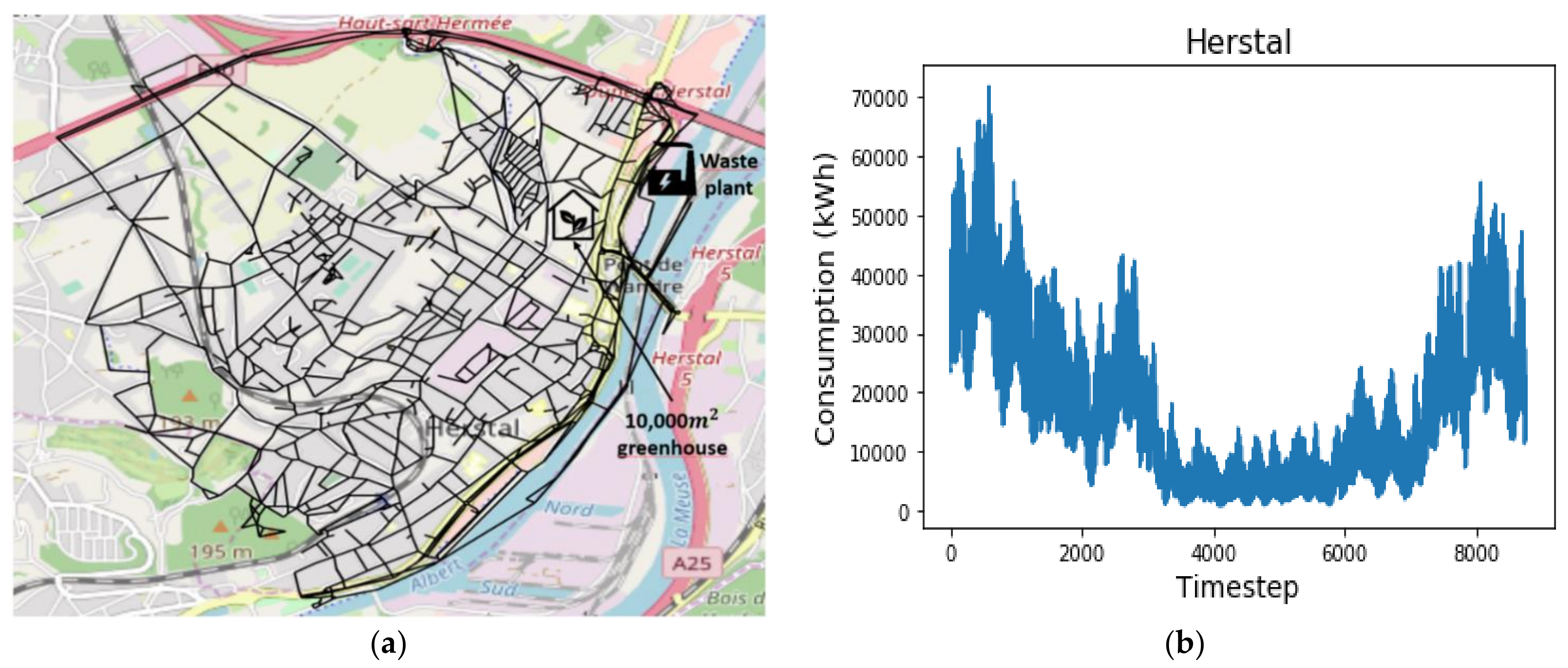
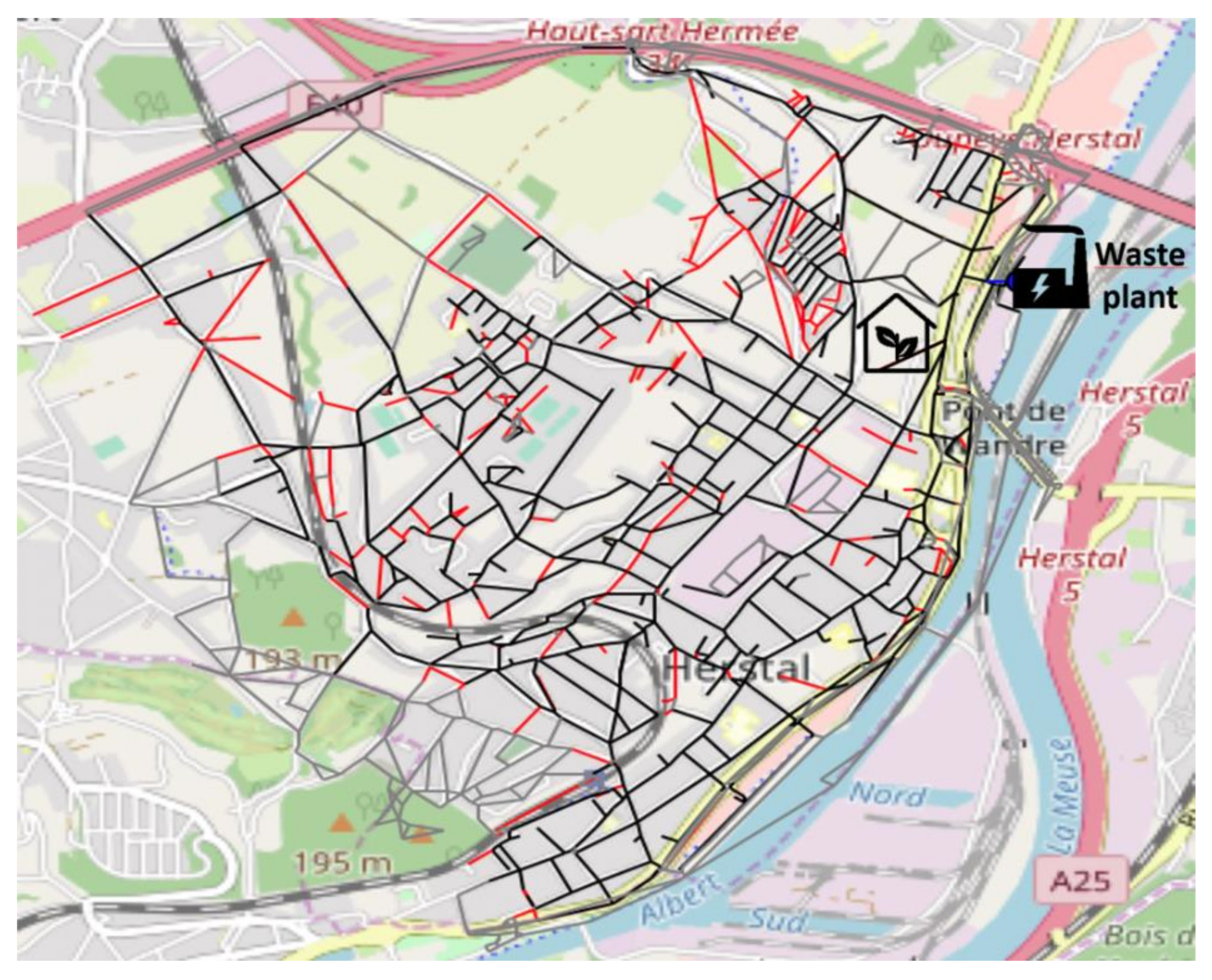
This optimization is achieved in this paper through a multi-period mixed-integer linear optimization model taking into account a set of constraints linked to the outline and the sizing of district heating networks. The multi-period feature of the model enables the ability to take into account the temporal behaviour of the heating load on a whole year, and, therefore, to efficiently integrate thermal storage solutions into the optimal solutions. The development of this optimization model is in line with a research project aiming to study the integration of a heating network into a prescribed geographic area with around 2000 streets in the city of Herstal (Belgium), represented in Figure 1, using a waste incinerator with a maximum thermal capacity of 100 MWth and a heating production cost of 0.03 €/kWhth. The possible inclusion of a 10,000 m2 greenhouse as a new heating consumer into the area is also considered. This project is looking for the economic and environmental benefits that could be derived from the implementation of a heating network based on the current scenario in competition using a decentralized heating production scheme with gas boiler units.

Figure 1.
(a) Large-scale case-study with nearly 2000 streets. (b) Total heating demand of this case study.
2. Problem Statement
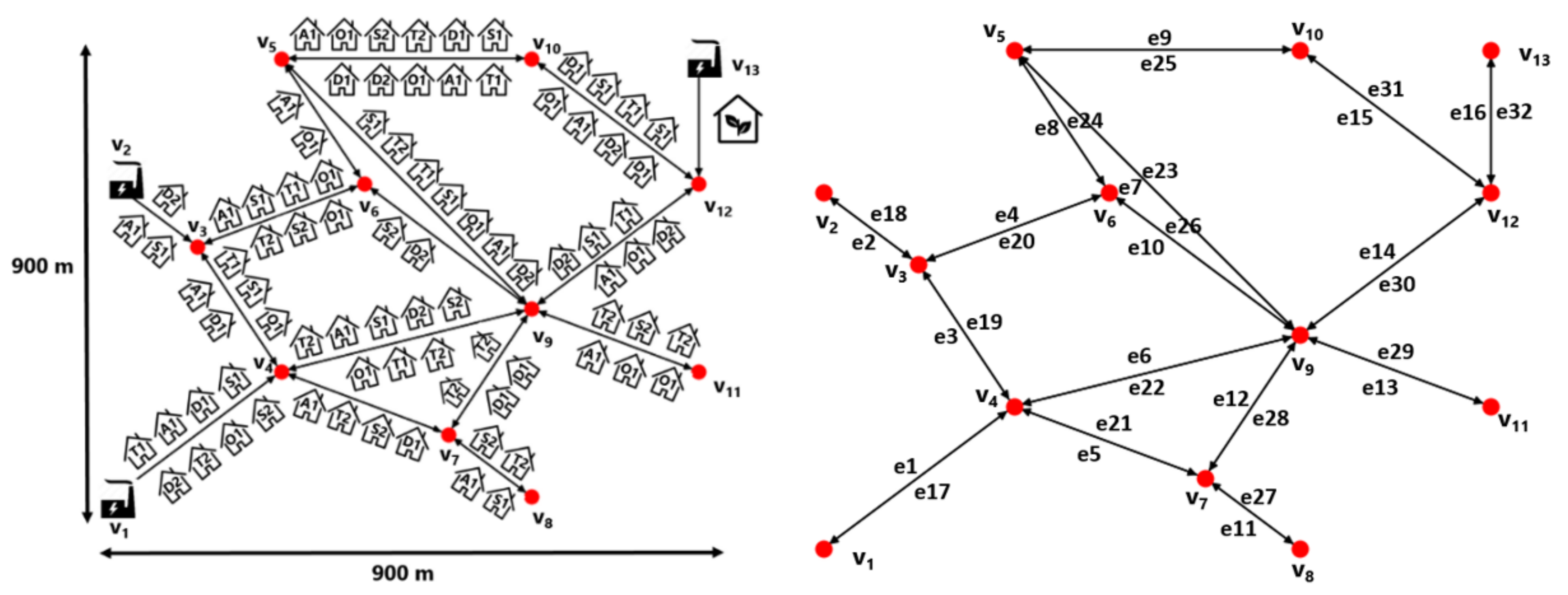
From this case study, an optimization formulation relying on a graph representation of the area defined in a geographic information system is developed in this paper. Edges e of the graph match with the streets of the studied area and their intersections are represented by the vertices v of the graph. As a first step, a small neighborhood with 16 streets and 3 potential heating sources based on the initial case is used as a small-scale test case as represented in Figure 2. This small case study enables the ability to define the formulation of the problem and to illustrate the main features of the optimization model, including the definition of the optimal outline of the network as well as the sizing of the different components constitutive of the network. The replication of the optimization formulation can then be demonstrated with the real case study for which the optimization tool is originally dedicated to. This real case study is made up of 1780 edges (of which 866 are heating consumers) and 1296 nodes, implying a large number of optimization variables requiring an adequate formulation of the optimization problem, ensuring a trade-off between numerical robustness and accuracy. From this graph representation, a set of vertices and edges is defined such that balance equations with some constraints are applied on the potential network to build.
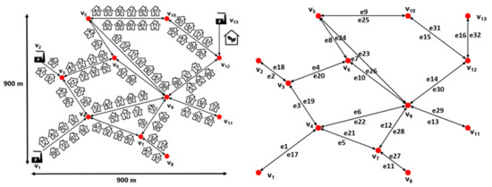
Figure 2.
Graph representation of a neighborhood of 16 streets with 13 intersections.
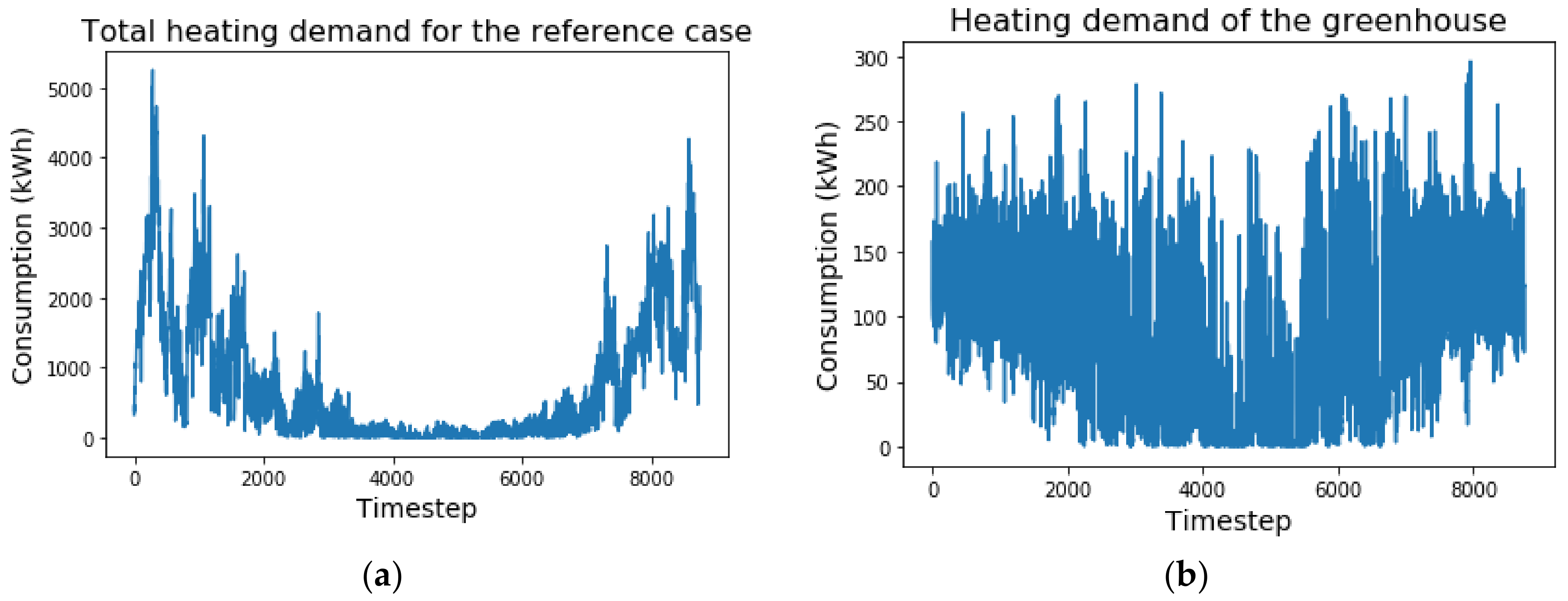
This case study includes buildings with different heating profiles and different levels of insulation. The total heating demand over the year of the whole neighborhood, including the heating demand of the greenhouse, is represented in Figure 3a. The specific heating demand of the greenhouse is exhibited in Figure 3b, illustrating the interesting heating profile of these kinds of consumers with a constant non-zero heating demand over the year. Different scenarios can then be studied to illustrate the influence of some parameters on the outline and the sizing of the network.

Figure 3.
(a) Hourly heating demand of the neighborhood. (b) Hourly heating demand of the greenhouse.
The reference scenario considers three existing available heating sources at nodes v1, v2 and v13 with a sufficient heating capacity to feed the whole heating demand of the network. The heating sales price is based on a market approach comparing alternative competitor’s prices. For the heating sector, the main competitors are the gas companies, such that the heating sales price with a heating network are based on the average gas price in the European Union, which is around 0.07 €/kWh. Heating sales prices between 0.07 €/kWh and 0.04 €/kWh are then considered for the reference scenario and the features of the three available heating sources are summarized in Table 1.

Table 1.
Features of the available heating sources.
Considering a prescribed project lifetime of 30 years with an actualization rate of 1% and assuming that all the potentials consumers on a given street would be connected to the network if a pipe is built on this street, a fair comparison from a current decentralized heating production scenario with gas boilers to a centralized heating production scenario using a heating network can be achieved using the optimization method developed in this paper.
2.1. Literature Review
District heating network technology is being studied more and more in the literature for its potential in the framework of the energy transition. Many studies are performed on the dynamic modelling and predictive control of operating district heating networks [8,9,10,11,12,13], while other works are related to the optimization of the outline and the design of these networks. Indeed, among the studies about the optimization of the outline and the design of district heating networks, Apostolou [14] develops a methodology based on a mixed integer non-linear (MINLP) optimization approach minimizing the total costs of the system for the integration and the design of heating and cooling sources into a new district heating or cooling project. A MINLP formulation based on the minimization of the total costs is developed by Mertz [15] for the outline and the whole sizing of a district heating project with the specificity to design the kind of connection between consumers (either parallel or in cascade). Roland [16] implements a mixed-integer nonlinear optimization model, taking into account a high level of details with all the hydraulic and thermal effects based on the Euler momentum and thermal energy equations.
Multi-objective non-linear optimization problems based on heuristic formulations are also developed to minimize total costs combined with a minimization of the CO2 emissions [17,18,19,20] or the share of primary energy import into the network [21]. These optimization formulations have a high level of complexity, enabling a detailed modelling of the system, but their multi-objective feature does not ensure a unique optimal solution for the problem. Furthermore, non-linear models are harder to solve, which limits the size of instances that can be tackled compared to linear ones.
Mixed integer linear programming formulations optimizing the design and operation of district heating systems [22,23] are also developed but do not define the optimal outline of a new district heating network project. These models are useful to assess the optimal use of existing heating sources, but the important aspect of which pipes and heating plants to build at given locations is missing. Some other models taking into account the optimization of the outline of the heating network exist in the literature. Some of these models [24,25,26] define the optimal outline of a potential network by choosing the consumers to connect, but are based on existing heating power plants with prescribed fixed capacities. The sizing of new potential heating plants is not included in these models.
Haikarainen [27] and Soderman [28] develop MILP approaches combining the optimization of the outline and the design/operation of the network but validate their models only on small test cases which are not connected to a geographic information system. Finally, Dorfner [29] implements an optimization formulation based on a geographic information system and combining both the outline and the design of a potential new heating network project. However, this model does not include thermal storage capacities and multi-source potential into the outline of the network. A summary of the different optimization models mentioned above and their main features is presented in Table 2 with the aim to identify the main features of each model available in the literature and highlight the missing features of these models compared to the one presented in this paper.
Table 2.
Review of the existing optimization methods.
The 6 features listed in Table 2 are assessed by the authors to be required, at least, to solve the problem introduced in Section 1. The optimization tool in this paper looks for determining the optimal outline and sizing of any new large-scale heating network from a geographic information system (GIS) for non-constant operating conditions in a quick way. Linear formulations generally guarantee a faster resolution and more numerical robustness than non-linear ones, especially for large-scale problems, such that an increase of the number of optimization variables does not generally impact the problem solving [30]. Regarding the multi-period feature of the proposed formulation combined with the study of thermal storage potential, it enables optimizing the outline and the sizing of the network for variable operating conditions providing a more accurate sizing of the different components of the network based on real heating consumption profiles.
The contribution of this paper with the new model described in the following sections is to fill in all the features presented in Table 2. The three main features combined in this new model are the following:
- A mixed-integer linear programming (MILP) model applicable from small-scale to large-scale case studies. The linearity of the model ensures a unique solution and guarantees robustness;
- A model combining both the optimization of the outline and the design of the network to map and size any new heating network project from scratch;
- A model that can be connected to a geographic information system and applicable to any new geographic area with potential consumers to connect to a network.
The main novelty of this optimization model relies on the range of problems that can be solved. Indeed, regarding the contributions available in the scientific literature, there are no optimization models able to deal with the outline and the sizing of large-scale heating networks with thousands of streets. This paper aims to fill this gap by applying the optimization model presented in this paper to a large-scale case study in a geographic area with nearly 2000 streets.
2.2. Methodology
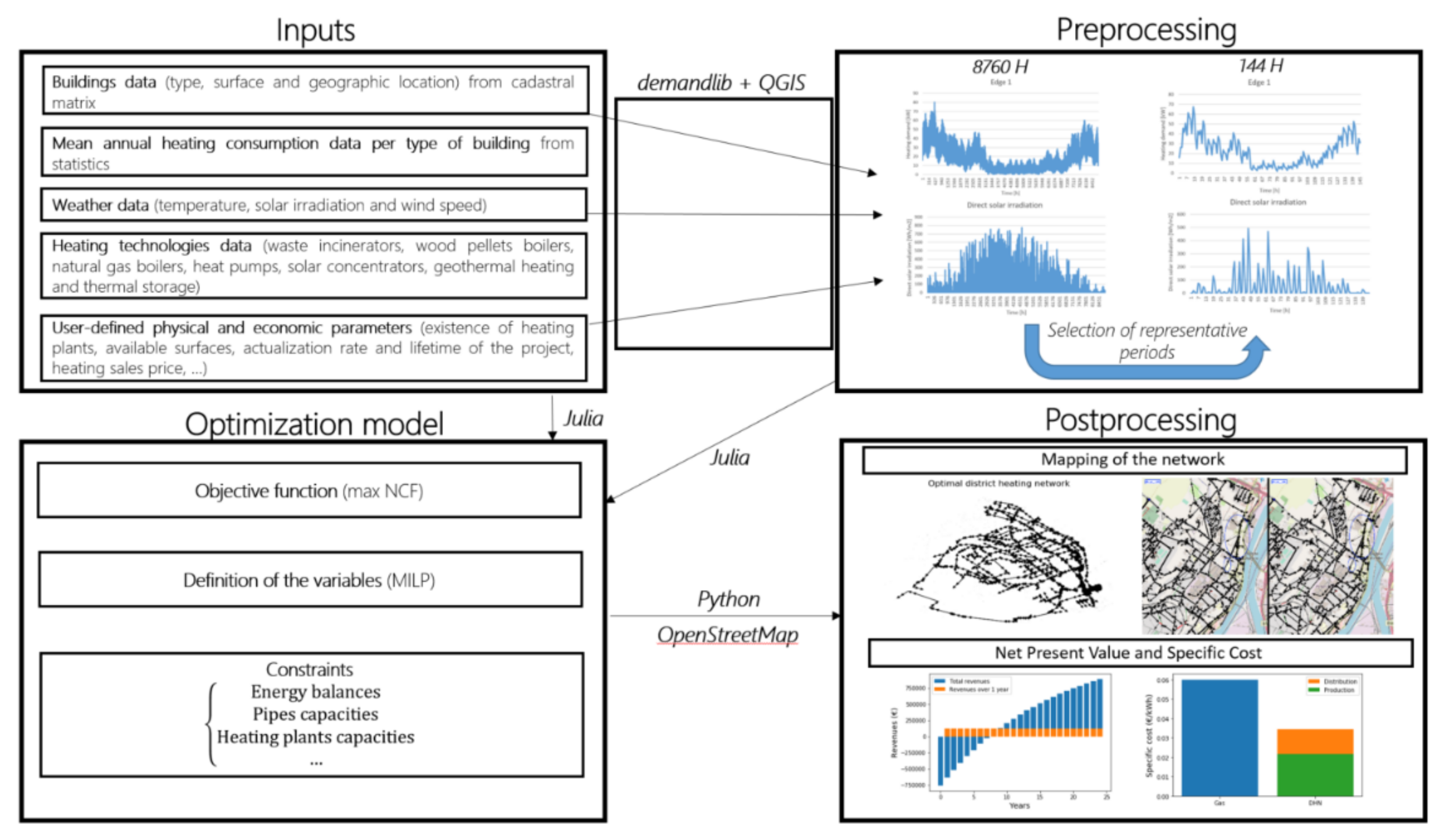
The architecture of the decision tool, represented in Figure 4, is based on a geographic information system intended to select a specific area for the implementation of a potential heating network. For any location, the geographic information system lists all the buildings with their features such as their type, their surface, their exact location and the street to which they are related to. The estimation of the hourly heating demand of each building is then computed from statistics data and the demandlib library in Python [31].

Figure 4.
Architecture of the decision tool.
National statistics listing the total heating consumption in Belgium for different sets of dwellings enable assessing the heating demand per square meter of a building of a given type in the country based on this total consumption in Belgium for each set of buildings. This heating demand per square meter is then used with the buildings data to compute the annual heating demand of any building knowing its total surface and its type. The next step of the heating demand estimation consists in distributing the annual heating demand over the year on hourly timesteps with the demandlib library. This Python library takes into account weather data, information about the building and the annual heating consumption of the building to generate an hourly heating demand. Finally, a heating demand profile is created for each building and each building is related to a specific street. A global hourly heating consumption file for each street is then generated.
The multi-period feature of the optimization formulation in this paper enables defining strategies for the sizing and operation of storage technologies. However, an optimization formulation based on an hourly time scale is very time consuming, especially for large-scale case studies. As illustrated in Figure 4, these hourly heating demands per street are then not directly used in the optimization model. There is a pre-processing of these profiles to select representative periods out of the year to reduce the number of timesteps to process into the optimization problem. This pre-processing is useful to ensure the robustness of the optimization model for large-scale problems by reducing the number of optimization variables.
An existing mixed integer linear optimization method developed by Poncelet et al. [32] is used and adapted to keep the temporal aspect of the heating demand as close as possible to the hourly heating demand and to include peak demands into the new generated synthetic year. The selection method is used to select 2 representative days per month and to add a third day for each month which is the day with the peak demand over the month. Weights wd and wt are then assigned respectively to each representative day and to each timestep of the representative days to create a new synthetic year to fit as accurately as possible the initial heating demand profile. Choosing 4 representative hours by representative day, a synthetic year with 36 representative days and 144 timesteps is finally generated and used as an input file for the optimization model written in the Julia language with the JuMP package.
The optimization model, described in the following section, aims to provide the optimal network architecture from linear constraints taking into account physical and urbanistic limitations for the studied area. A post-processing is then proposed to visualize the results of the optimization in a user-friendly way for the users of the decision tool.
2.3. Optimization Model
The model developed in this paper aims to maximize the net cash flow from a heating network while taking into account the main physical and urbanistic constraints related to its implementation. These constraints are based on the graph representation illustrated in Figure 2 which is used to define different sets of optimization variables.
2.3.1. Sets
Defining V as the set of indices i of all the vertices vi of the graph, another subset VP V containing the indices of the vertices vi which are potential heating plants and thermal storages locations is defined. For each vertex vi VP, a set Hi listing all the available technologies m for heating production is defined. This set of technologies includes waste incinerators, wood pellets plants, gas boilers, heat pumps, solar collectors, geothermal plants and thermal storages. All these vertices have to be linked by edges ej whose the indices j are included into a set E and additional sets of edges Ni include all the indices of the adjacent edges ej to a given node vi. Finally, a time component has to be taken into account to determine a multi-period optimization problem by defining a set T made up of Ntimesteps timesteps of a duration of hours, a set D containing all the Nreprday representative days d and subsets TD T containing Nreprhour timesteps t for a representative day d.
2.3.2. Constraints
We first define the constraints of the optimization problem. These constraints are defined in a general way based on physical conservation laws and on potential practical requirements. This generic definition of the constraints and their related variables enables applying the formulation for similar optimization purposes to any new heating network project.
Energy Balance at the Vertices and Edges of the Graph
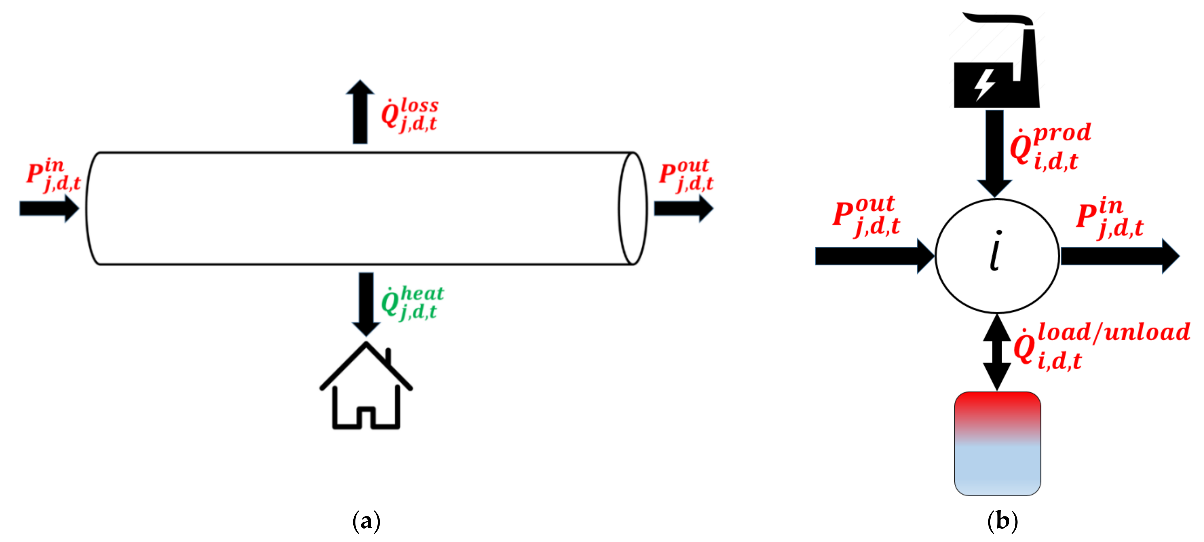
The first set of constraints deals with energy balance both on the edges and the nodes of the network. Energy flows are supplied by potential heating sources and/or thermal storages located at some vertices of the graph such that energy balances at the vertices and the edges of the graph are satisfied as illustrated in Figure 5.

Figure 5.
(a) Energy balance over an edge j. (b) Energy balance over a vertex i.
Based on this figure, an energy balance over each edge and node of the graph can be written as follows:
where are respectively the incoming and outcoming power flows into a pipe at edge characterized by a heating consumption weighted by a connection rate . This connection rate takes into account the ratio of consumers that would agree to be connected to the network. represents the heating production at a node , with the index i included into the subset VP, and are the loading and unloading power flows from a potential storage at this node. These 3 last variables are equal to zero if the index i is not included in the subset VP. The binary variable is required to define if a pipe is used or not at a given timestep.
Thermal losses are one of the main drawbacks of heating networks such that they have to be taken into account to define the best way to build and size the network. A heat transfer model based on [12] is used in this paper to define an analytical formulation of these heat losses taking into account losses between the supply and the return pipes with respective temperatures and as well as between the pipes and the surroundings with a temperature . Heat losses per unit length of pipe can then be directly computed from Equation (3).
Thermal resistances and are dependent on the pipe diameters, and each pipe diameter is dedicated to a specific range of power flows due to the limitation of the pressure losses into the pipes. Generally, a nominal value of 100 Pa/m related to a maximum power flow into the pipes is prescribed. Heat losses are a function of the pipe diameters as illustrated in Figure 6a. According to basic fluid mechanics [33], the pressure losses are directly proportional to the mass flow rate to the square and inversely proportional to the pipes diameters to the power 5. Heat losses defined by the variable can then be computed by linking the pipe diameters to the mass flow rates (and indirectly the power flows) for prescribed pressure losses as represented in Figure 6b.
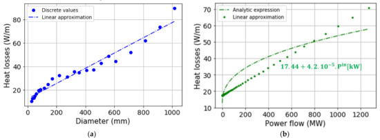
Figure 6.
(a) Heat losses as a function of pipes diameters. (b) Heat losses as a function of the power flows.
A linearization of the heat losses as a function of the power flows into a pipe of length gives an analytical formulation of the variable:
The binary variable defines the use or not of a built pipe at an edge ej during the time period t such that if the pipe is not used, there are no heat losses in the pipes. A piecewise linearization of the heat losses function could lead to a better approximation of this function. However, the piecewise linearization requires the definition of new binary variables for each pipe such that this formulation would be intractable, especially for large instances. Regarding thermal storages, they act as buffers to satisfy heating requirements that are not covered by heating production units at some time periods. These storages are used for shifting the heating production from a time period to another and can have an influence on the sizing and the operating conditions of the network. The integration of thermal storage units into the optimization model is thus achieved by defining loading and unloading storage variables but also a variable assessing the level of the storage in kWh at any time period. This variable is used for sizing the optimal thermal storage(s) volume(s) for a given network. Assuming a perfectly stratified storage with constant temperatures within the two laminate zones of water inside the storage tanks ( = 90 °C and = 60 °C), an energy balance over each time period enables linking the stored heating energy to the loaded or unloaded heating power by the storage units. We initialize the storage level to 50% of the maximum potential storage capacity which would be installed and prescribe that the initial and final storage levels at the end of the optimization period are equal (). Specifically, it can be written as:
is a parameter quantifying thermal storage losses from a time period to another one. Time-dependent heat losses of a water tank over time are computed considering transient conduction through the tank. An analytical formulation based on the lumped capacitance method making the assumption that the fluid temperature is spatially uniform at any moment during the transient process is used. Assuming an initial temperature in the tank, the temperature at a time t is given by:
where R is the thermal resistance to convection heat transfer and C is the lumped thermal capacitance of the water tank. Linking the sizing of the thermal storage to the available surface at a given location, a coefficient for hourly heat losses in nominal operating conditions can be defined as a function of the available surface at a potential storage location. From Equation (6), the temperature in the storage after an hour for an initial temperature can be computed assuming a thermal storage capacity of 35 kWh/m3 for a water temperature difference at the substations of 30 K:
Figure 7 illustrates the decrease of the heat losses coefficient for an increase of the available surface . This physical trend is explained by the decrease of the ratio between the heat exchange surface of the storage and the storage volume reducing then the heat losses per unit of stored heat. This heat loss coefficient can be linearized to keep a linear formulation of the problem.
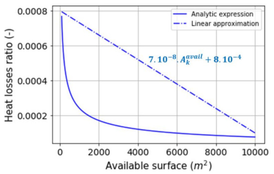
Figure 7.
Value of the heat losses coefficient as a function of the available surface.
Maximum Thermal Capacity on the Vertices and Edges of the Graph
Pipes’ diameters in the streets are generally limited by urbanistic constraints because of limited space in the ground due to the presence of other existing pipes, such as gas and telecommunication pipes. As explained in the previous section, the limited power flow can be linked to a maximum pipe diameter which can be installed into the ground such that a constraint about the maximum thermal power capacity for each pipe can be written as follows:
This set of constraints defines, at any time period, the power flow into a pipe of the network while verifying that the maximum thermal capacity on a street is not outreached. The binary variable defines whether a pipe at an edge ej is built or not.
Heating power capacities are also limited by the size of the available existing heating plants and by the potential available surfaces for the implementation of new heating sources at a prescribed node with the index i included into the subset VP. For new potential heating plants to install, their limited thermal capacity is computed from the required surface per unit of heating capacity available in [34] for a given technology m.
A parameter taking into account the variability of the heating capacity over time has to be defined, especially for the solar heating production capacity. The intermittency of the solar radiation is taken into account for the computation of the solar capacity production available with solar collectors with a prescribed inclination and orientation to determine the maximum installable capacity and the available capacity over each timestep of the year. The sizing of the solar collectors is based on the peak solar radiation in clear sky conditions determining which is used to define the capacity factor for solar technology for each time period:
Finally, the heating production level defined in Equation (2) for all the available heating technologies m can be linked to the heating production of each heating technology m at any timestep by defining the following constraint:
Link between Pipes over Some Edges of the Graph
The last set of constraints deals with the decision process of which pipes to build or not in the network. We have the following constraints:
Equation (14) allows for a degree of freedom regarding the decision to build some pipes. In the framework of political decisions linked to district heating projects, some consumers would have to be mandatorily included to the district heating project. The mandatory feeding of some consumers by a heating network is expressed by a binary parameter for each edge ej which has a value of 1 if the building of a pipe is mandatory over an edge ej and 0 otherwise. Equation (15) links the building of a pipe to its use such that a pipe can not be used if it is not built. Equation (16) links each edge ej of the directed graph with its equivalent edge in the opposite direction . It imposes the use of a pipe in a unique direction at any timestep.
2.3.3. Costs and Revenues
Costs related to a heating network can be divided into two main categories including capital and operating expenses. The different costs related to these two categories can be expressed as:
Capital expenditures are defined to be accounted for only at the beginning of the investment period while operating expenditure are taken into account during the whole lifetime of the project. Actualization factors are taken into account to include the value of money over time by means of an actualization rate a. The value of the actualization rate depends on the borrowing rate available on the markets, the debt to equity ratio of the borrowing company and the expected return on equity expected by the stakeholders of the project. This rate is generally particularly favorable to the development of district heating because district heating networks’ projects are considered as low risk assets and the current borrowing rates on the financial markets are low [35]. A general formula can be used to compute this actualization rate as following:
Based on these actualization factors and considering that there is no energy price inflation, the actualization factors are defined by Equations (20) and (21). The calculation of these actualization factors is based on the definition of the present value of a cash flow over time. This value corresponds to the market price today (time 0) of a monetary unit available at a future date time t.
Capital expenditures represent all the building costs linked to the best-suited outline and sizing of the network project. These costs are considered to be achieved at the beginning of the project (year 0) and are assessed based on current market prices. The building and operation of heating power plants depend on some parameters determining the kind of power plant and the capacity to install, or to use if the heating plant is already in operation. Based on data from [34] for different heating technologies, a coefficient [€/kWth] for cost per unit of installed capacity for technology m can be defined to compute a heating plant building cost function. This cost coefficient is equal to zero in the case of an already existing power plant.
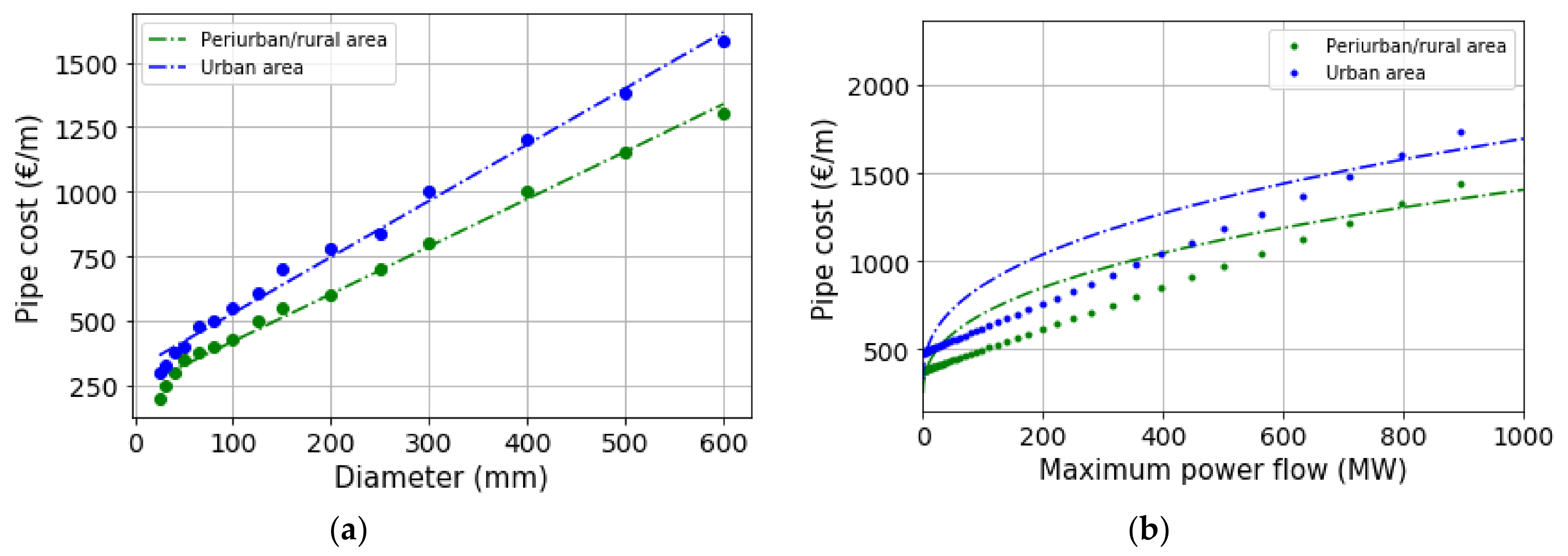
For heating networks operating at temperature levels between 60 and 100 °C, pipes are generally made up of steel surrounded by a polyethylene foam insulation. The costs of these pipes and their implementation are dependent on their diameters and the location of the pipes. The setting up of pipes in an urban area is more expensive than in a periurban or rural area. These costs are represented graphically in Figure 8a and are linked to the maximum power flow into the pipes as for the heat losses. This non-linear relation represented graphically in Figure 8b can be linearized over the range of power flows between 0 and 1 GW. The linear expression for these pipe costs is then given by Equations (23) and (24).
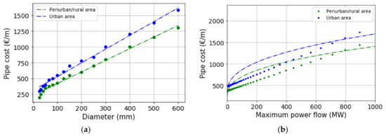
Figure 8.
(a) Pipes costs as a function of pipes diameters. (b) Pipes costs as a function of the power flows.
The binary variable is used to define a pipe cost function per meter of pipe only if the pipe is built. Otherwise, this cost becomes zero. The definition of the pipe cost function relies on this linearization of the pipes’ costs per unit length and depends also on the length Lj of each edge of the potential network and of the location of the pipe in an urban or periurban/rural area defined respectively by both binary parameters and . These binary parameters have a value of 1 if the edge locates respectively in an urban or periurban/rural area and zero otherwise. The global pipe cost function is thus defined by Equation (25).
Considering that one substation is installed per built pipe, the sizing of these substations is based on the maximum heating demand over an edge. Substation costs are directly proportional to their heating capacity such that a linear expression of the substations cost per thermal unit installed is defined as follows:
This cost depends on the parameter of connection percentage representing the ratio of inhabitants over an edge which agree to be connected to a district heating network. This parameter is used to take into account that in real district heating projects, some inhabitants are opposed to the project and want to keep their current heating system at home. The global cost function for substations is then defined as follows taking into account which edges are connected to the network:
Similarly to the definition of a cost function for the heating plants, the computation of the thermal storages costs are based on data from [34] defining a coefficient [€/kWhth] for costs per unit of installed storage.
Operating expenditures represent all the ongoing costs to operate the network based on the determined sized components. These costs are considered to be achieved continuously over the lifetime of the project and are neglecting any energy inflation assuming a constant energy price over the years. Heating production costs have to be computed over each timestep of the optimization period taking into account the heating production level of each heating technology m at each heating location k. These production levels are linked to a time-dependent parameter because the heating production cost of some technologies, such as heat pumps, are dependent on external time dependent factors, such as the electricity price and weather conditions impacting the coefficient of performance of this technology. A generic formulation of the costs for heating production is given by Equation (29).
For the heat pump technology, the assessment of the parameter is based on a polynomial laws’ model to assess the coefficient of performance of a heat pump (HP) for a given level of temperature at the condenser prescribed by the operating temperature of the heating network and an hourly prescribed electricity price for a reference year. Combining the coefficient of performance COPd,t of the heat pump with the electricity price , the heating cost with a heat pump technology can be directly computed as follows:
Water circulation over the network requires pumping power to satisfy the heating requirements at each timestep of the optimization problem. These pumps are fed by electricity such that the pumping power is dependent on the electricity price and the power flow into a pipe. The electrical consumption of a pump circulating a fluid with a mass flow rate considering unit pressure losses into the pipe is given by Equation (31):
Considering nominal pressure losses with a prescribed pump efficiency (75%), the electrical consumption over any edge ej can be computed. The global pumping cost function including the pumping consumption over all the edges of the network is then defined as follows:
Finally, revenues from heating sales are the main income. Contracts for heating sales can take various forms from one district heating project to another. However, pricing models are generally based on a market approach for private owners projects and on a cost approach for municipal owners projects [5] to define the total heating bill of the consumer. In the case of a new district heating project, the revenue component is based on a fixed heating price per unit of heat consumed. Total heating revenues are computed over the whole network based on potential heating consumptions as defined in Equation (33):
The main goal of the optimization tool defined in this paper consists of providing the network’s outline with the best-suited heating technologies and thermal storages to maximize profits over the lifetime Nyears of a given district heating network project. The total cost of the project and its revenues thus has to be computed over the entire lifetime of the project to define the optimization function maximizing the net cash flow (NCF):
3. Results
3.1. Reference Scenario
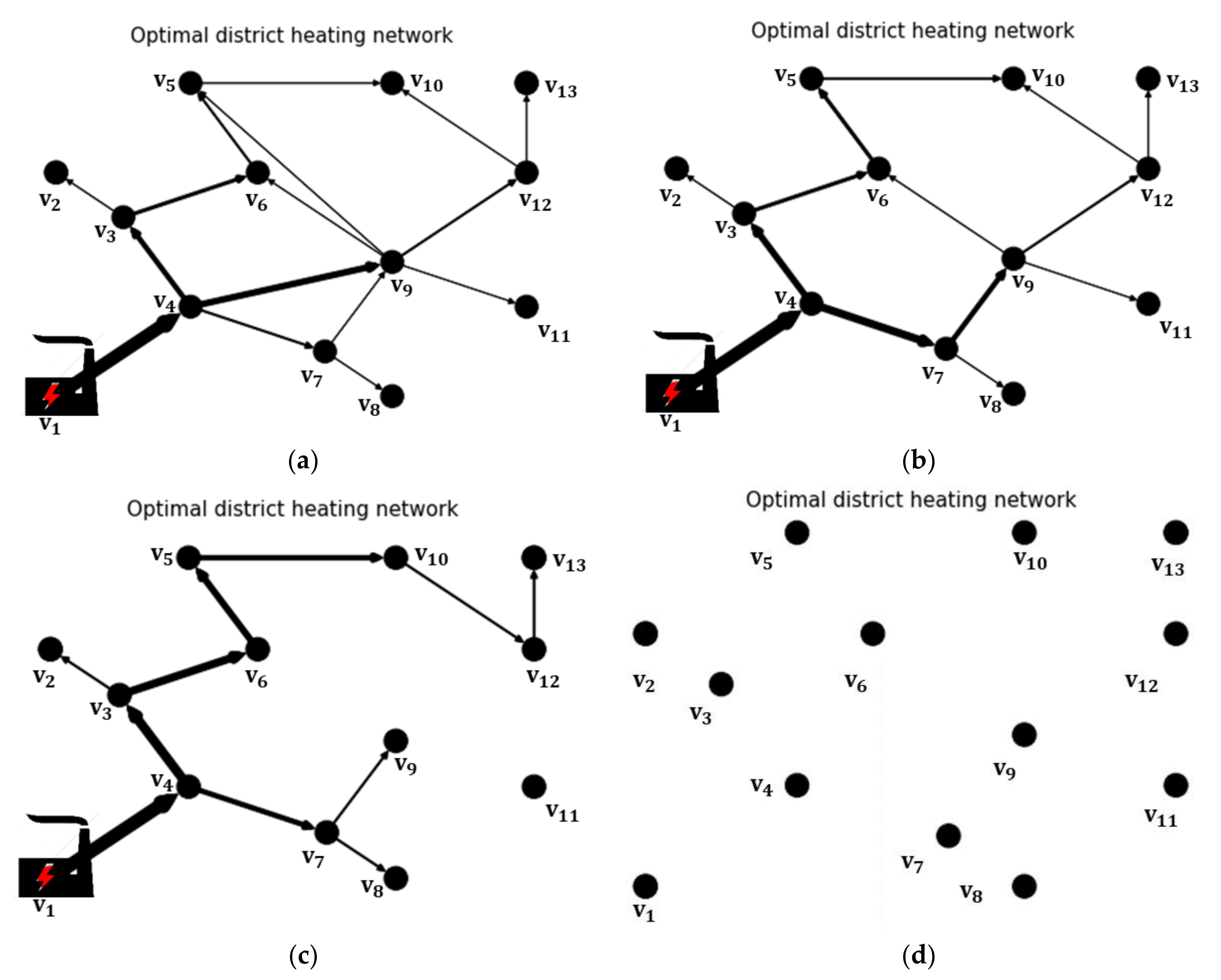
Considering the initial case study described in Section 2, the model contains 35,111 variables and is solved using the Gurobi solver with an optimality gap of 0.1%. The computations are executed in 25 s on a computer with an Intel® Core™ i7-8650U processor with 8 threads at 1.90 GHz and 16GB RAM. With a project lifetime of 30 years and an actualization rate of 1% assuming that all the potentials consumers over a given street would be connected to the network if a pipe is built into this street (), results for different heating sales prices starting from the heating sales price of a decentralized scenario (rheat = 0.07 €/kWh) are illustrated in Figure 9.

Figure 9.
(a) rheat = 0.07 €/kWh; (b) rheat = 0.06 €/kWh; (c) rheat = 0.05 €/kWh; (d) rheat = 0.04 €/kWh.
It can be observed from Figure 9 that it is profitable to build a heating network with a unique heating source at node v1 with the cheapest production cost of 0.03 €/kWh. Compared to a decentralized heating production scenario with a same heating cost of 0.07 €/kWh, the heating network project remains profitable. The most interesting conclusion to draw from this reference scenario is the influence of the heating sales price on the outline of the network. The decrease of the heating sales price reduces the number of streets connected to the heating network such that only the most financially interesting consumers are connected.
The decrease of these heating revenues can also be illustrated in Figure 10 with the decreasing net present value of the optimal network project defined by the optimization for these different heating sales prices.
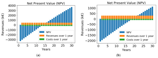
Figure 10.
(a) rheat = 0.07 €/kWh; (b) rheat = 0.05 €/kWh.
The decrease of the heating sales price increases the payback period of the project such that this period is respectively of 11, 13 and 18 years for heating sales prices from 0.07 €/kWh to 0.05 €/kWh. The optimization model is thus useful to determine a sufficiently high heating sales price to generate profits for the district heating network project.
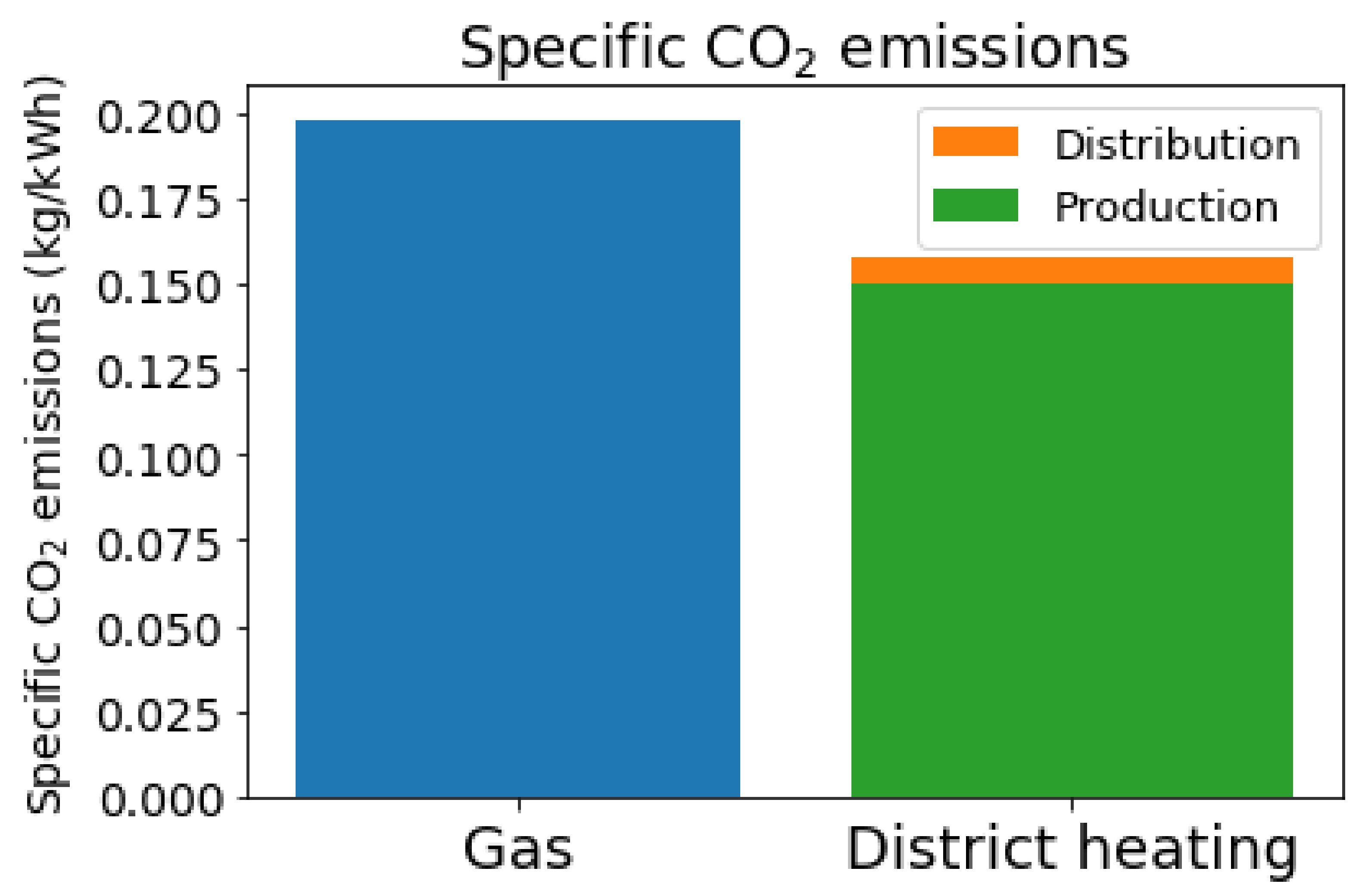
Regarding the CO2 emissions with a heating network using the heating source at node v1 compared to the use of decentralized gas boilers in each house of the network, the building of a heating network leads to a decrease of 24% of CO2 emissions as illustrated in Figure 11. CO2 emissions for the heating network includes the emissions linked to the required production to satisfy the heating demand but also the additional heating production to fulfil heat losses linked to the heating distribution between the production unit and the consumers.
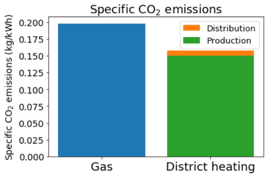
Figure 11.
Specific CO2 emissions with a heating network and decentralized gas boilers.
Based on this reference scenario, the influence of some main parameters defined in Section 2 for a heating network implementation is analyzed in the following sections.
3.2. Influence of the Limited Maximum Diameters in the Streets
As explained previously, the thermal capacity in some edges of the network are sometimes limited by the space in the ground needed to put a new pipe along the street. Considering a case where the edges 6 and 22 defined in Figure 2 between nodes v4 and v9 are constrained by a zero thermal capacity (), the new optimal outline for the network is shown in Figure 12.

Figure 12.
Influence of the limitation of some pipes diameters.
A zero thermal capacity between nodes v9 and v12 influences the outline of the network, and also the thermal power plant capacity used and the profits made out of the heating sales. Due to the non-supply of the street between these 2 nodes, the total heating demand to satisfy decreases and implies a reduction of the thermal capacity to use of 455 kWth and also the profits generated from incomes by heating sales with a decrease of profits of 62,000 €.
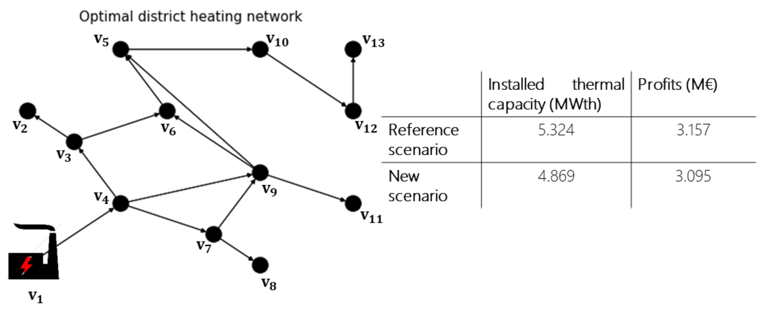
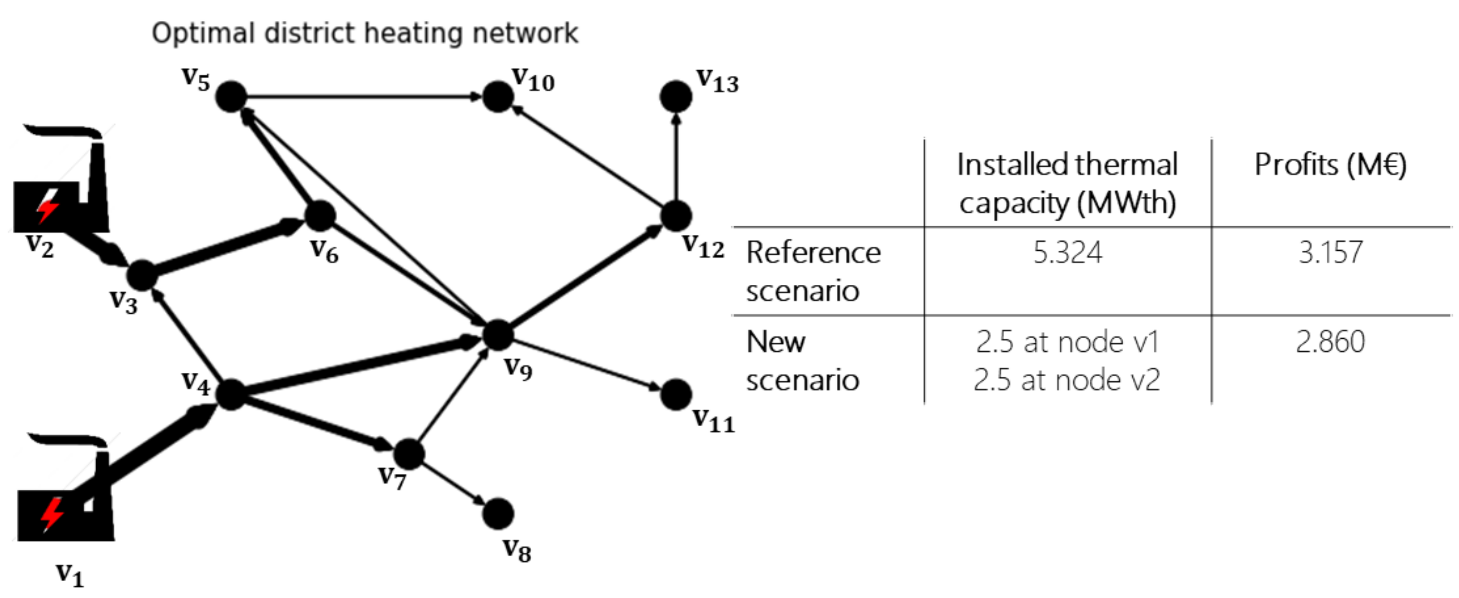
3.3. Influence of the Limited Thermal Capacities at the Power Plants
Decreasing the maximum thermal capacities of each plant from 10 MWth to 2.5 MWth such that the 3 heating plants could be used in order to satisfy the whole heating demand, the new design of the outline of the heating network is depicted in Figure 13 with the use of the maximum capacity of the plants only at nodes v1 and v2 of 2.5 MWth. The limited capacity at the thermal plants prescribes the use of 2 plants to satisfy a part of the heating demand while staying financially profitable. The peak heating demand over the year is larger than 5 MWth (cf. Figure 3), but the plant at node v13 to cover the rest of the heating demand is not used due to the heating production cost being too expensive in this plant compared to the profits generated from heating sales with this heating plant.
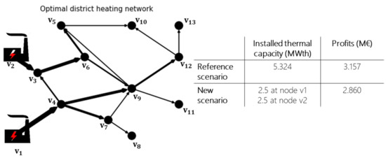
Figure 13.
Influence of the limitation of the heating capacities of the power plants.
It can also be noticed from Figure 13 that the use of a second more expensive heating source decreases the total profits from the heating network because of a higher heating production cost and lower profits because the heating demand is not wholly met due to the limited total heating capacity.
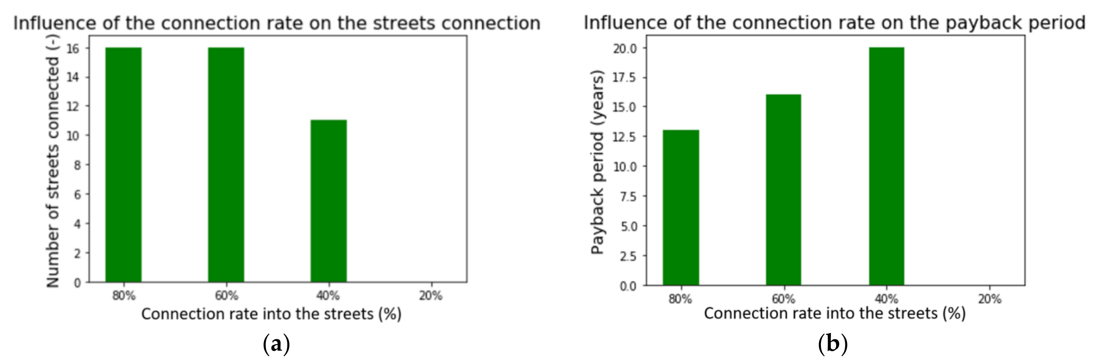
3.4. Influence of the Connection Rate on a Street
Another important parameter influencing the outline and the sizing of the network takes into account the connection rate of the consumers over each street of the network. The connection of a consumer to a network on a street depends on the choice of the consumer to be connected or not. In the reference scenario, a case with a maximum connection rate () is considered, while in practice, this connection rate is rarely 100%. A parametric study of the influence of this connection rate on the outline and the sizing of the network is achieved in this section with a connection rate decreasing from 100 to 20%.
As illustrated in Figure 14, the decrease of the connection rate reduces the number of streets connected to the network and extends the payback period. For a connection rate of 20%, it is no longer of interest to build a heating network in the studied area.

Figure 14.
(a) Number of streets connected; (b) payback period.
3.5. Influence of the Actualization Rate of the Project
The type of financing for heating networks also influences the outline and the sizing of the network. An increase of the actualization rate raises the amount of cash flow in the form of interests due to the stakeholders of the project. An accurate assessment of the actualization rate of the project remains essential in order to not underestimate some additional costs which could make the network non profitable to build and operate. As depicted in Figure 15, a slight increase of the actualization rate could lead to a non-profitable heating network such that a decentralized heating solution would then be preferred.
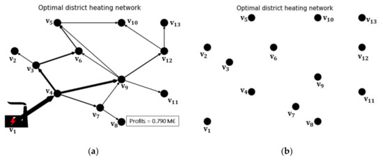
Figure 15.
(a) a = 2%; (b) a = 3%.
3.6. Design from Scratch and Integration of Thermal Storage Solutions
Previous scenarios consider existing heating sources with a constant heating production cost without any available surface for the building of a new heating source or a thermal storage. Thermal storages can be really useful in the design of heating networks designed from scratch for some cases, such as those listed below:
- A shift of the heating production from periods of high production costs to periods of low production costs. Technologies, such as heat pumps, have a heating production cost dependent on the electricity price and its coefficient of performance. It could be optimal to produce heat during periods of low heating production costs periods and store the additional heat not required to satisfy the heating demand into thermal storages;
- A match between the heating production and the available heating capacity for intermittent energy sources, such as solar collectors, for example. Intermittent heating sources may not always provide the heating demand due to a fluctuating limitation of their capacities. A part of the heating production has thus to be shifted from periods with a low heating capacity to periods with a larger heating capacity and stored thanks to the use of thermal storages;
- An undersizing of the heating plant capacity to build in order to reduce capital expenses. The use of a thermal storage can decrease the sizing of the heating capacity of the plants by producing more constantly over the year and storing the additional heating production into a thermal storage during low heating demands periods. This stored heat can then be unloaded during periods of high heating demand when the heating plant may not guarantee a sufficient capacity to feed the whole network.
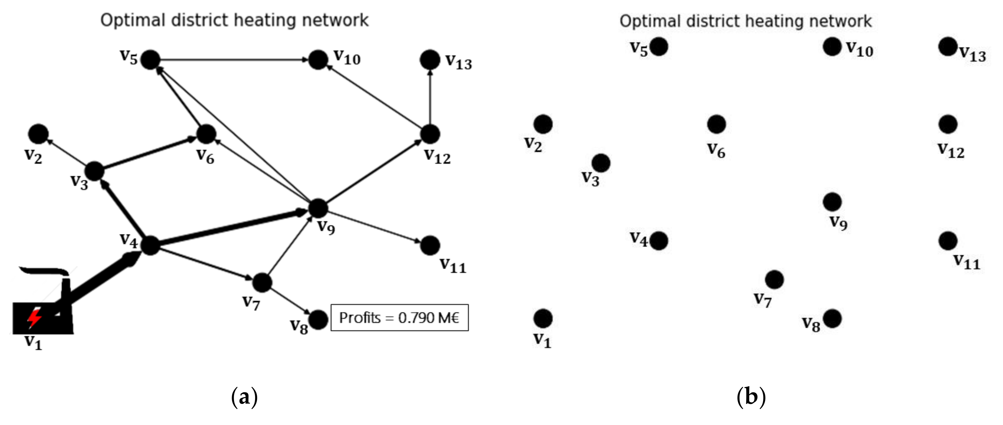
In this section, the building of a heating network from scratch is considered and the influence of the inclusion of a thermal storage unit into the network is studied. This scenario aims to define the optimal trade-off between a minimization of the capital and operating expenses related respectively to the building of new plants and the heating production while maximizing revenues by selling heat to the consumers. Considering three available surfaces of 1000 m2 at nodes v1, v2 and v13 for the building of new heating plants and thermal storages, the optimal outline and design of a heating network is depicted in Figure 16.
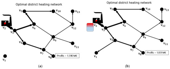
Figure 16.
(a) Optimal outline without storage capacity. (b) Optimal outline with storage capacity.
Both cases, without thermal storage solutions and with thermal storage solutions, are characterized by the building of heating plants and storages at node v2, respectively. The optimization tool defines the best location for the building of new heating plants in order to minimize the operating costs linked to heat losses and pumping power. The inclusion of thermal storage solutions enables connecting all the streets to the network and to increase profits related to heating sales by approximately 15%.
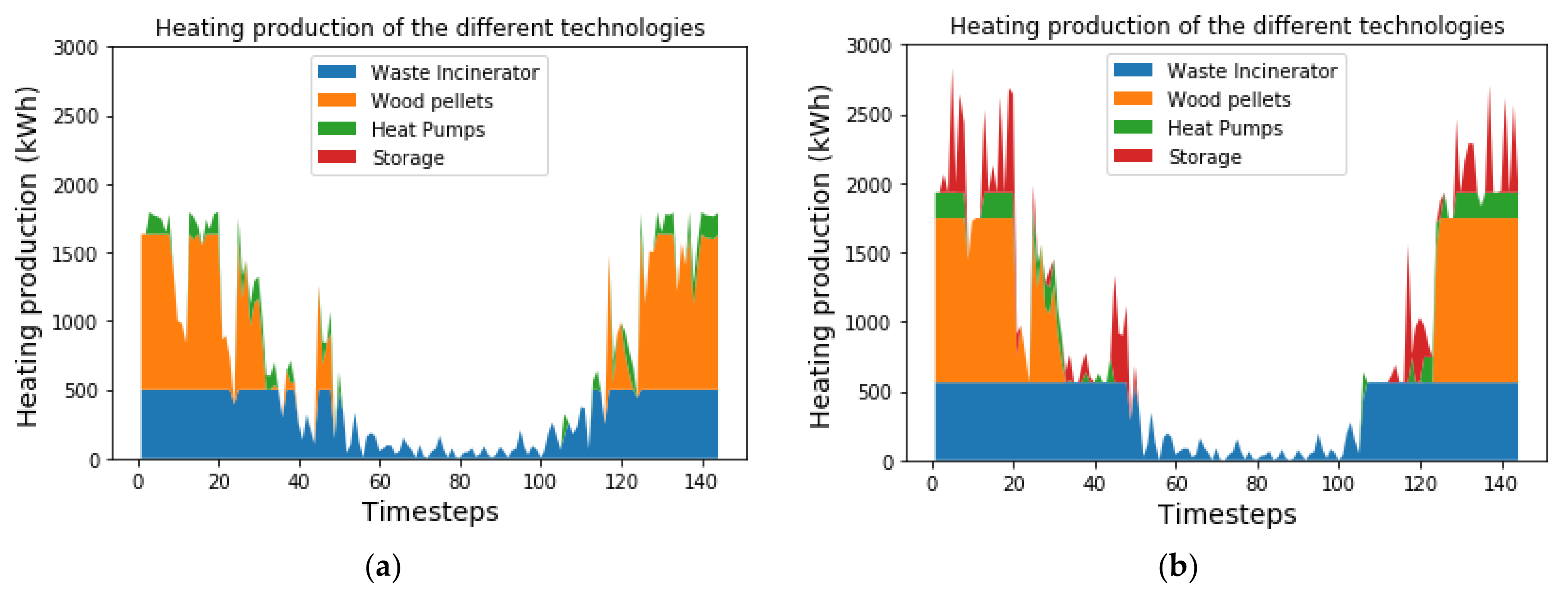
Regarding the heating production profiles in Figure 17, the optimization model enables selecting the optimal heating sources for base load production and peak load production. A waste incinerator with low heating production costs (0.03 €/kWh), but larger capital building costs (2500 €/kW), is used for the base load production with an installed capacity of 500 kWth. A wood pellets plant, characterized by lower building costs (600 €/kW), but a larger heating production cost (0.04 €/kWh), is built with a capacity of 1100 kWth to satisfy the additional heating demand. Finally, heat pumps are used as a back-up technology which is used during periods of low heating production costs with an installed capacity of 150 kWth. The inclusion of a thermal storage with a capacity of 13.3 MWh into the network enables taking advantage of the use of the heat pumps with variable heating production costs by storing heating production from the heat pumps and using this stored heat during periods of high heating demands.
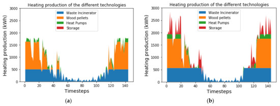
Figure 17.
(a) Heating production without storage capacity. (b) Heating production with storage capacity.
4. Application of the Tool to the Large-Scale Initial Case Study
The main goals of the optimization tool developed in this paper consists of determining the consumers to connect to the real case of a new heating network project in the city of Herstal and studying the influence of the integration of a 10,000 m2 greenhouse on the profitability of the project. The greenhouse might be an interesting consumer to integrate into the new network thanks to its little fluctuating heating consumption over the whole year, and especially because of the non-zero heating demand during the summer. The optimization formulation is used to determine the optimal outline and design of the optimal heating network that could be built in the studied area. For this case study, the model contains 2,808,510 variables and is solved using the Gurobi solver with a larger optimality gap than previously of 5% in order to limit the computation time of the problem due to the large number of variables. The computations are executed in 4465 s on a calculation server with 48 Intel® Xeon® E7 v4 2.20 GHz processors with a total RAM of 126 GB.
A project lifetime of 30 years with a constant heating sales price of 0.07 €/kWh is considered assuming that all the potential consumers over a given street would be connected to the network if a pipe is built into this street (). The optimal outline of the network is exhibited in Figure 18 inspired from [36] from the same authors.
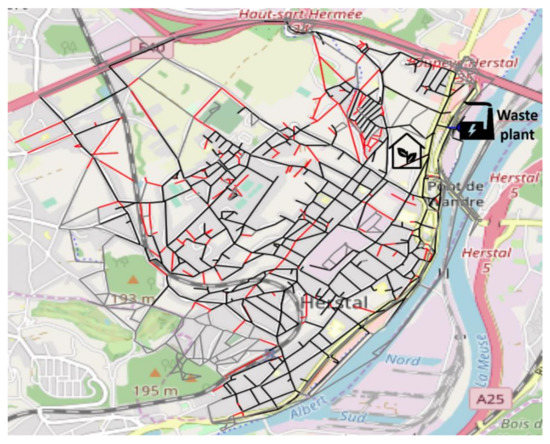
Figure 18.
Optimal outline of the Herstal heating network.
The decision tool determines the mapping of the optimal heating network. It can be observed in Figure 18 that most heating consumers edges (806 out of 866 edges), depicted in black, are connected to the network while some others, depicted in red, are not integrated into the heating network because they are assessed to be non-economically profitable to connect. These streets are related to additional investment and operating costs that are not counterbalanced by the revenues generated from the heating sales.
Results concerning the influence on the sizing of the network for the integration of a greenhouse are summarized in Table 3. The connection of the greenhouse to the network also slightly increases the capital and operating expenses linked respectively to the building of a new pipe and substation to connect the greenhouse to the network while increasing the total heating production to supply the additional heating demand of the greenhouse. However, the additional revenues generated from the heating sales to the greenhouse are larger than the additional costs such that the inclusion of a greenhouse as a new heating consumer remains economically profitable. Regarding the environmental benefits, the use of a heating network to supply heat to the consumers of the studied area might reduce the CO2 emissions by 24%. The heating network sized from the optimization model thus has economic and environmental benefits compared to a decentralized heating production with gas boiler units.
Table 3.
Main outputs of the optimization model for the Herstal case study.
5. Conclusions and Perspectives
This paper presents a multi-period mixed-integer linear programming optimization model which is part of a decision tool that can be useful for project leaders and policymakers. This tool can be used for the optimal outline and sizing of any new heating network project defined with some streets in a geographic information system by selecting the consumers to connect and by sizing the different components required for the building of this network. One of the novelties in this paper based on the existing literature review lies in the range of applications that can be solved with a very limited computation time, from 25 s for a small-scale case study with 35,111 optimization variables to only around one hour for a large-scale case study (around 2000 potential streets to connect) characterized by 2,808,510 optimization variables.
The user-defined approach of the decision tool allows defining different personalized scenarios for a given network project in order to perform a sensitivity analysis regarding economic and urbanistic parameters. Best practice rules based on empirical data can then be substituted or enhanced by the use of this optimization tool to determine break-even points below which it is no longer profitable to build a heating network. A sensitivity analysis for the case study presented in this paper exhibits that a heating sales price below 0.05 €/kWh, an actualization rate for the project above 2% or a connection rate on a street below 40% does not guarantee any more profitability for a 30-year project lifetime.
The multi-period feature of the optimization model provides thermal storage solutions to increase the available total thermal capacity through the network. The integration of a thermal storage solution in a new heating network project enables increasing the number of connected streets to the network while increasing the total profits made up from the network by approximately 15%. Considering non-constant operating conditions in the optimization formulation also enables defining an optimal set of heating technologies respectively for base load and peak load heating production compared to a single period optimization model. Another goal of this work relies on the integration in heating networks of specific heating consumers, such as greenhouses with a constant non-zero heating demand, to improve their profitability. Even though the connection of these new kinds of consumers to the network implies additional costs, surplus revenues from these financially interesting heating consumers guarantee a profitable investment.
Finally, the linear formulation of the model provides a trade-off between acceptable computation times and sufficient accuracy, especially for large-scale case studies, for assessing the optimal outline and sizing of new heating network projects. However, piecewise linear or non-linear formulations might be adapted from the formulation proposed in this paper to increase the accuracy of the formulation proposed in this paper even though there would be no more guarantees for finding a feasible solution in acceptable computation times. In addition to studying the influence of the formulation on the optimization results and the computation time, the authors would like to apply the presented model to other heating network projects with new user-defined parameters in order to check the optimization method, and to help policymakers and investors to identify profitable heating network projects.
Author Contributions
T.R.: Conceptualization, Methodology, Validation, Writing—Original Draft Preparation. Q.L.: Writing—Reviewing and Editing. P.D.: Writing—Reviewing and Editing, Supervision, Funding acquisition. All authors have read and agreed to the published version of the manuscript.
Funding
This research was supported by the European Union and the Walloon region with the European Funds for Regional Development (EFRD) in the framework of the VERDIR Tropical Plant Factory (Project EcoSystemPass) grant number 1510610.
Conflicts of Interest
The authors declare no conflict of interest. The funders had no role in the design of the study; in the collection, analyses, or interpretation of data; in the writing of the manuscript, or in the decision to publish the results.
References
- Mathiesen, B.V.; Lund, H. Global smart energy systems redesign to meet the Paris Agreement. Smart Energy 2021, 1, 100024. [Google Scholar] [CrossRef]
- Connolly, D.; Lund, H.; Mathiesen, B.V.; Werner, S.; Möller, B.; Persson, U.; Boermans, T.; Trier, D.; Østergaard, P.A.; Nielsen, S. Heat roadmap Europe: Combining district heating with heat savings to decarbonise the EU energy system. Energy Policy 2014, 65, 475–489. [Google Scholar] [CrossRef]
- Fleiter, T.; Elsland, R.; Rehfeldt, M.; Steinbach, J.; Reiter, U.; Catenazzi, G.; Jakob, M.; Rutten, C.; Harmsen, R.; Dittmann, F.; et al. Profile of heating and cooling demand in 2015, Deliverable D3.1 Report, Heat Roadmap Europe 2017. Available online: https://heatroadmap.eu/wp-content/uploads/2018/11/HRE4_D3.1.pdf (accessed on 30 August 2021).
- European Commission. An EU Strategy on Heating and Cooling. 2016. Available online: https://eur-lex.europa.eu/legal-content/EN/TXT/PDF/?uri=CELEX:52016DC0051&from=EN (accessed on 30 August 2021).
- Werner, S. International review of district heating and cooling. Energy 2017, 137, 617–631. [Google Scholar] [CrossRef]
- Andrews, D.; Pardo-garcia, N.; Krook-Riekkola, A.; Tzimas, E.; Serpa, J.; Carlsson, J.; Papaioannou, I. Background Report on EU-27 District Heating and Cooling Potentials, Barriers, Best Practice and Measures of Promotion. Joint Res. Centre 2012. Available online: http://www.diva-portal.org/smash/get/diva2:994924/FULLTEXT01.pdf (accessed on 30 August 2021).
- International Energy Agency. Governance Models and Strategic Decision-Making Processes for Deploying Thermal Grids Governance Financial. 2017. Available online: http://www.districtenergy.org/HigherLogic/System/DownloadDocumentFile.ashx?DocumentFileKey=e24e4c4e-3cd8-825e-d1eb-518dc945632c&forceDialog=0 (accessed on 30 August 2021).
- Laajalehto, T.; Kuosa, M.; Mäkilä, T.; Lampinen, M.; Lahdelma, R. Energy efficiency improvements utilising mass flow control and a ring topology in a district heating network. Appl. Therm. Eng. 2014, 69, 86–95. [Google Scholar] [CrossRef]
- Dobos, L.; Abonyi, J. Controller tuning of district heating networks using experiment design techniques. Energy 2011, 36, 4633–4639. [Google Scholar] [CrossRef]
- Jie, P.; Zhu, N.; Li, D. Operation optimization of existing district heating systems. Appl. Therm. Eng. 2015, 78, 278–288. [Google Scholar] [CrossRef]
- Guelpa, E.; Barbero, G.; Sciacovelli, A.; Verda, V. Peak-shaving in district heating systems through optimal management of the thermal request of buildings. Energy 2017, 137, 706–714. [Google Scholar] [CrossRef] [Green Version]
- Sartor, K.; Quoilin, S.; Dewallef, P. Simulation and optimization of a CHP biomass plant and district heating network. Appl. Energy 2014, 130, 474–483. [Google Scholar] [CrossRef] [Green Version]
- van der Zwan, S.; Pothof, I. Operational optimization of district heating systems with temperature limited sources. Energy Build. 2020, 226, 110347. [Google Scholar] [CrossRef]
- Apostolou, M. Méthodologie Pour la Conception Optimisée des Réseaux de Chaleur et de Froid Urbains Intégrés.HAL Id: Tel-02274400. Université de Recherche Paris Sciences et Lettres Préparée à MINES ParisTech Méthodologie. 2019. Available online: https://pastel.archives-ouvertes.fr/tel-02274400/document (accessed on 30 August 2021).
- Mertz, T.; Serra, S.; Henon, A.; Reneaume, J.M. A MINLP optimization of the configuration and the design of a district heating network: Academic study cases. Energy 2016, 117, 450–464. [Google Scholar] [CrossRef]
- Roland, M.; Schmidt, M. Mixed-integer nonlinear optimization for district heating network expansion. At-Automatisierungstechnik 2020, 68, 985–1000. [Google Scholar] [CrossRef]
- Falke, T.; Krengel, S.; Meinerzhagen, A.K.; Schnettler, A. Multi-objective optimization and simulation model for the design of distributed energy systems. Appl. Energy 2016, 184, 1508–1516. [Google Scholar] [CrossRef]
- Fazlollahi, S.; Becker, G.; Ashouri, A.; Maréchal, F. Multi-objective, multi-period optimization of district energy systems: IV—A case study. Energy 2015, 84, 365–381. [Google Scholar] [CrossRef]
- Molyneaux, A.; Leyland, G.; Favrat, D. Environomic multi-objective optimisation of a district heating network considering centralized and decentralized heat pumps. Energy 2010, 35, 751–758. [Google Scholar] [CrossRef]
- Weber, C.; Shah, N. Optimisation based design of a district energy system for an eco-town in the United Kingdom. Energy 2011, 36, 1292–1308. [Google Scholar] [CrossRef]
- van der Heijde, B.; Vandermeulen, A.; Salenbien, R.; Helsen, L. Integrated optimal design and control of fourth generation district heating networks with thermal energy storage. Energies 2019, 12, 2766. [Google Scholar] [CrossRef] [Green Version]
- Bertrand, A.; Mian, A.; Kantor, I.; Aggoune, R.; Maréchal, F. Regional waste heat valorisation: A mixed integer linear programming method for energy service companies. Energy 2019, 167, 454–468. [Google Scholar] [CrossRef]
- Omu, A.; Choudhary, R.; Boies, A. Distributed energy resource system optimisation using mixed integer linear programming. Energy Policy 2013, 61, 249–266. [Google Scholar] [CrossRef]
- Bordin, C.; Gordini, A.; Vigo, D. An optimization approach for district heating strategic network design. Eur. J. Oper. Res. 2016, 252, 296–307. [Google Scholar] [CrossRef]
- Maria Jebamalai, J.; Marlein, K.; Laverge, J.; Vandevelde, L.; van den Broek, M. An automated GIS-based planning and design tool for district heating: Scenarios for a Dutch city. Energy 2019, 183, 487–496. [Google Scholar] [CrossRef]
- Samsatli, S.; Samsatli, N.J. A general mixed integer linear programming model for the design and operation of integrated urban energy systems. J. Clean. Prod. 2018, 191, 458–479. [Google Scholar] [CrossRef]
- Haikarainen, C.; Pettersson, F.; Saxén, H. A model for structural and operational optimization of distributed energy systems. Appl. Therm. Eng. 2014, 70, 211–218. [Google Scholar] [CrossRef]
- Söderman, J.; Pettersson, F. Structural and operational optimisation of distributed energy systems. Appl. Therm. Eng. 2006, 26, 1400–1408. [Google Scholar] [CrossRef]
- Dorfner, J.; Hamacher, T. Large-scale district heating network optimization. IEEE Trans. Smart Grid 2014, 5, 1884–1891. [Google Scholar] [CrossRef]
- Luenberger, D.; Ye, Y. Linear and Nonlinear Programming; International Series in Operations Research and Management Science; Springer: Berlin/Heidelberg, Germany, 2016; ISBN 9780387745022. [Google Scholar]
- Hilpert, S.; Kaldemeyer, C.; Krien, U.; Günther, S.; Wingenbach, C.; Plessmann, G. The Open Energy Modelling Framework (oemof)—A new approach to facilitate open science in energy system modelling. Energy Strateg. Rev. 2018, 22, 16–25. [Google Scholar] [CrossRef] [Green Version]
- Poncelet, K.; Hoschle, H.; Delarue, E.; Virag, A.; Drhaeseleer, W. Selecting representative days for capturing the implications of integrating intermittent renewables in generation expansion planning problems. IEEE Trans. Power Syst. 2017, 32, 1936–1948. [Google Scholar] [CrossRef] [Green Version]
- Werner, S. District Heating and Cooling. In Reference Module in Earth Systems and Environmental Sciences; Elsevier: Amsterdam, The Netherlands, 2013. [Google Scholar]
- The Danish Energy Agency. Energinet Technology Data—Generation of Electricity and District Heating. 2016. Available online: https://ens.dk/en/our-services/projections-and-models/technology-data/technology-data-generation-electricity-and (accessed on 30 August 2021).
- ADEME. Les Réseaux de Chaleur et de Froid—État des Lieux de la Filière. 2019. Available online: https://librairie.ademe.fr/energies-renouvelables-reseaux-et-stockage/818-reseaux-de-chaleur-et-de-froid-etat-des-lieux-de-la-filiere-marches-emplois-couts.html (accessed on 30 August 2021).
- Résimont, T.; Thomé, O.; Joskin, E.; Dewallef, P. Tool for the Optimization of the Sizing and the Outline of District Heating Networks using a Geographic Information System: Application to a Real Case Study. In Proceedings of the ECOS 2021—The 34th International Conference On Efficiency, Cost, Optimization, Simulation and Environmental Impact of Energy Systems, Taormina, Italy, 27 June–2 July 2021. [Google Scholar]


Publisher’s Note: MDPI stays neutral with regard to jurisdictional claims in published maps and institutional affiliations. |
© 2021 by the authors. Licensee MDPI, Basel, Switzerland. This article is an open access article distributed under the terms and conditions of the Creative Commons Attribution (CC BY) license (https://creativecommons.org/licenses/by/4.0/).