Bayesian Inference of Dwellings Energy Signature at National Scale: Case of the French Residential Stock

Abstract

Cities take a central place in today’s energy landscape. Urban Buildings Energy Modeling (UBEM) is identified as a promising approach for energy planning and optimization in cities and districts. It generally relies on the use of Building Archetypes, i.e., simplified deterministic models for categorized building typologies. However, this implies large assumptions which may accumulate and induce significant bias on energy consumption estimates. In this work, we address this issue with static stochastic models whose parameters are inferred over national thermo-energy data using Bayesian Inference. We analyze inference results and validate them with a panel of standard indicators. Then, we provide comparative results with deterministic building archetypes and stock data from the TABULA European project. Comparisons between heat loss coefficients show relative coherence between building categories, but highlight some significant bias between both approaches. This bias is also shown in the comparative result of a Monte Carlo simulation using inferred stochastic models for a 10331 dwellings stock. In conclusion, inferred stochastic models show interesting insights over the French dwellings stock and potential for district energy simulation. All code and data involved in this study are released in an open repository.

1. Introduction

1.1. Estimating Dwellings Consumption at District Scale

1.1.1. Context

To address energy transition challenges, most actions nowadays are intended towards electric production and grid, energy usage in buildings and transportation. For the production part, renewable energy is one of the main development axes and will lead to a deeper decentralization of the electric grid and new challenges due to its intermittent nature. For the consumer part, efforts aim to reduce the use of fossil energy and increase efficiency.

All these actions greatly increase the energetic complexity in urban areas if one wants to globally integrate environmental incentives and regulations. As stated in [1], intermittent load fluctuations induced by PV systems and electric vehicles can compromise the grid stability if taken independently, but this effect could be avoided with an appropriate synchronous management of both.

Besides, many studies account buildings for $30\%$ to $40\%$ of energy consumption in most developed countries [2], and therefore play a critical role in aforementioned challenges.

It is realistic to say that many buildings won’t be replaced but simply refurbished to comply with new environmental directives. The refurbishment strategy must be cost-effective and give priority to the less efficient buildings and preferably target households facing energy insecurity (or “fuel poverty”, mostly due to the conjunction of low income with low building energy efficiency). Therefore, it is essential to be able to simulate and assess the energy load in urban areas at various levels.

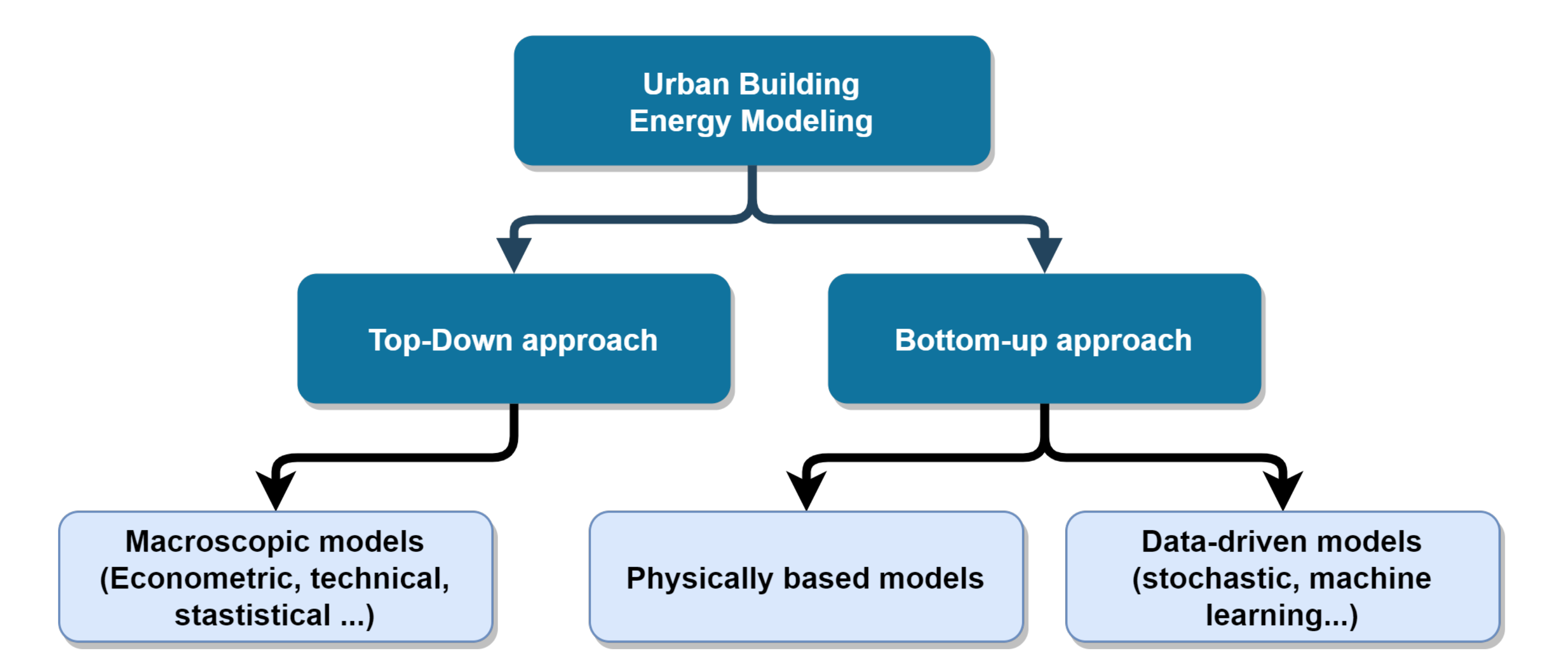
1.1.2. Approaches and Models for Urban Energy Assessment

To address these issues, intensive work is led towards data availability and openness, alongside with software solutions to model districts and process related data. More and more cities, countries, national companies and international organizations are providing datasets under open-source licensing. Such data can be leveraged at city scale to help assess and increase the energy efficiency with a better transparency, but can still lack standardization policies [3,4]. In the case of Europe and France, we can cite some databases relevant for energy and building studies in

Table 1. Open data sources examples for energy and buildings.

Name	Contents	References
European Urban Data Platform Plus	Provides access to information on the status and trends of cities and regions and to EU supported urban and territorial development strategies. This application enables studies up to regional scales.	[5]
TABULA/EPISCOPE	Launched in 2012, European projects EPISCOPE and TABULA aggregate results of detailed studies for the residential stock of 16 European countries. The database offers two main products: the TABULA Webtool as an endpoint for representing typical buildings per country and categories, and all technical reports from consultants implied in the project.	[6,7]
ENEDIS Open Data platform	Electric and Gas consumption data aggregated at various scales from ENEDIS (ex-ERDF), the Power Grid Operator in France.	[8]
ADEME Open Data platform	ADEME—The French Agency for Ecological Transition, provides about 112 datasets as of 2021 related to the energy transition in France	[9]
Open Platform of French public data	The French Government gathers in this platform most data issued from public services and affiliated companies. Most datasets are released under the “Licence Ouverte/Open License” licensing.	[10]
Data portals for major cities	Most important urban areas in Europe provide open data related to urban space use and major local events.	Examples: city of Grenoble [11], Lyon [12] and Paris [13]

.

If such data can be used “as is” in statistical studies, they can also feed energy models for more advanced inferences and predictions. Such models can produce valuable insight for urban energy planning. For example, projects such as HotMaps [14,15] or PLANHEAT [16] are starting to use open data at European scale through energy mapping tools.

In the case of the residential sector, modeling approaches are classified in the literature between bottom-up and top-down categories [17], as depicted Figure 1.

Top-down strategies are mostly used at a macroscopic scale (coarse variables at national/international scales), and try to use simple models such statistical regression to link energy consumption with macro-economic indicators at a national scale. However, their use is limited in time because based on historical data. They are less prone to provide detailed insights due to their macroscopic nature, but in conjunction with GIS data, a good spacial resolution can be reached as shown in [18]. Conversely, bottom-up approaches try to start from detailed models to describe the stock and compute energy consumption by aggregation. To do so, we can use physically based models (white-box), data-driven models (black-box) or anything in-between (mixed/hybrid models). Many bottom-up tools for Urban Buildings Energy Modeling (UBEM) rely on the concept of “building archetypes” or typologies to deal with data lacunarity and modeling complexity.

Table 2. City and district buildings modelers examples.

Name	Features	References
City Energy Analyst	This stand-alone open-source tool aims to target several aspects of district modeling and energy demand forecasts. It provides a “data helper” to leverage some included datasets (mostly concerning Switzerland) and helps to generate building models using 15 typologies.	[21]
TEASER	TEASER is an open-source Python package to generate Modelica models of buildings based on “Buildings” and “AixLib” Modelica libraries. A building model can be generated with few parameters such as the construction date and the net leased area, using pre-defined typologies and default values partially issued from TABULA.	[22]
City BES	City Building Energy Saver is web-based tool leveraging GIS and building datasets (CityGML) to generate EnergyPlus models at district scale, themselves used for benchmarking and energy load prediction.	[23]
City SIM	City SIM helps the user to model 3D buildings and various flows at district scale. It features a specific focus on radiative modeling and use of climate boundary conditions.	[24]

lists some of these tools with a specific focus on physical models. For extensive reviews of bottom-up UBEM tools, the interested reader can refer to [19,20].

The main idea behind this concept of archetypes is to cluster the building stock in a handful of representative typologies. Each model corresponding to a typology can be tuned by a minimal set of parameters such as the net floor area or the number of floors. With statistical expansion (i.e., on populated enough areas), the modeler expects individual errors to cancel-out each other in the total sum of the energy load.

Such approach is very practical considering the current state of district scale datasets. The modeler directly feeds the modeling tool with available data, and missing parameters are defaulted or computed by specific rules. Since each building is modeled individually, it is easier to change parameters and therefore estimate the overall impact of new policies or refurbishments, which is not possible with aggregated top-down models. For example, one can modify insulation parameters of a range of buildings to estimate the investment return of an insulation campaign.

1.2. Issues with District Energy Models Using Deterministic Archetypes

During the construction of a district energy model from deterministic building archetypes, issues may arise due to the nature of underlying data and strong model hypotheses:

• From the authors experience, even when using archetypes with few input parameters, getting reliable data is still a challenge. Indeed, available data at district scale is generally sparse and heterogeneous, if not erroneous. Besides, open data is aggregated to comply with privacy requirements of citizens, it is therefore difficult to directly access detailed, individual data. Furthermore, most buildings don’t have an energy model available for reuse. Only most recent buildings used building energy simulation in the conception phase, and such models are most of the time not publicly available (e.g., proprietary). In [19], lack of data and underlying algorithms is also pointed out as an important issue in residential energy consumption estimation through bottom-up building stock models.
• The use of standard/default parameters and model structures may lead to accumulated biases. To give a simple example, if we consider a district with one dominant typology and architectural characteristics, initial bias on thermal parameters in buildings models may accumulate and lead to significant error in the total energy load. In a previous work, we study thermal flexibility at district scale with such approach and point out important errors between archetype models using the same data sources [25].

One approach to deal with these problems is to use optimization and calibration strategies. For example, in [26], the author proposes a recursive optimization algorithm to select a limited set of building model archetypes such as the predicted energy mix matches measured national consumption.

Considering the high uncertainty levels in the field of UBEM, new studies start to address the issue through statistical methods and stochastic modeling. Ref. [27] points out the problem of uncertainties management as a major limitation, and proposes a review of stochastic approaches as an alternative.

The major advantage of stochastic models towards deterministic ones lies in their ability to account for uncertainties and their propagation. Two main approaches can be found: the Frequentist and the Bayesian. The Frequentist is the traditional one. It generally uses maximum likelihood estimation (MLE) methods to identify moments of probability density functions (pdf), optimization methods such as least squares in linear regression, and statistical tests to assert similitude or differences between measured random variables. For example, in Pasichnyi et al. [28], the authors illustrate a data-driven approach in the case of Stockholm leveraging Energy Performance Certificates and energy signatures for archetypes buildings estimated using linear regression on individual consumption profiles. The Bayesian approach however is based on the propagation of probability distributions across models by exploitation of the well-known Bayes’s rule. By design, it helps to incorporate prior knowledge in the model and regularize the parameters’ estimation problem. Estimation results can be represented as distributions and therefore integrate uncertainties from models and data. According to Lim et al. review [27], this approach is becoming quite popular in buildings model calibration and UBEM. Other studies such as [29] on a residential case study in Kuwait City, suggest good performances in calibration compared to deterministic or uncalibrated stochastic approaches. Refs. [30,31] also illustrate and validate the interest of Bayesian calibration for the most uncertain parameters in building archetypes, for the respective residential cases of Amsterdam and Cambridge, Massachusetts.

1.3. Objectives and Structure of the Paper

1.3.1. Contribution

Since the Bayesian approach enables the integration of prior knowledge, hierarchical model structures with nested distributions, it appears to be a promising framework to the definition of stochastic archetypes models for UBEM, enabling a better management of uncertainties while preserving physical sense of resulting models.

Our work aims to study the feasibility of such approach in the case of simple dwelling models, and to compare produced results with the more traditional approach of deterministic archetypes.

To do so, we use geographically aggregated data to reconstruct a set of simple categorized physical models (i.e., archetypes) which could be used in bottom-up studies at urban scale. We apply here the Bayesian Inference framework on energy signature models for dwellings using French national scale databases. The major goal is to have access to distributions of base and thermosensitive energy consumption in dwellings categorized by their type, construction date and habitable surface. This can be seen as a disaggregation of energy data that would hardly be usable in bottom-up models otherwise. Since the used models have a physical sense, they could be updated empirically for specific cases (e.g., insulation improvements), or directly from local data thanks to the Bayesian framework.

In a second part, we compare inferred physical parameters (heat loss coefficients) with the corresponding ones used in the building archetypes provided by the European TABULA project. Results show coherent values variations across dwelling categories, but highlight a significant bias between both approaches linked with refurbishment hypotheses in TABULA models. We also illustrate how our inferred stochastic models can be used in Monte Carlo simulations at district scale. Such simulation highlight the cumulative consequences of biases between stochastic and deterministic archetypes.

1.3.2. Structure of the Paper

This paper is composed of three major sections:

• In the first one, we introduce the Materials and Methods used in our work. More specifically, we present our test case of the French residential stock and the associated datasets. We explain how data is constituted and pre-treated to suit our needs. Then, we describe the model of energy signature used all along this work and the stochastic model and algorithms used to perform inference over our data.
• In the second one, we expose and interpret inference results for three variants of our inference model, each variant corresponding to an increase of the number of dwelling categories. Convergence and validation of the inference process is detailed and validated using state-of-the-art indicators.
• The third one is the comparative study with results from the TABULA project previously mentioned. This study relies on comparative box plots for heat loss coefficients and a Monte Carlo simulation from inferred models.

To conclude, we discuss on the potential advantages and limitations of the use of stochastic Bayesian archetypes in the field of UBEM, and highlight axes for follow-up studies.

2. Materials and Methods

2.1. Case Study: Dwellings “Energy Signature” over Metropolitan FRANCE

2.1.1. Model of “Energy Signature” for a Building

The “energy signature” model is one of the simplest we can conceive for a building. It has a major advantage of requiring few measurements (Mains power consumption and external temperature). This model will be involved in both datasets and inference steps. In the case of a building with only heating and no cooling, we can observe a linear dependency of daily energy consumption with outdoor average temperature during cold months, and no dependency with temperature the rest of the time. In presence of a cooling system, we can observe a similar linear behavior for hot days. Therefore, we can model the daily energy demand by a piece-wise linear function. For a dwelling with no cooling, such model can be formulated by Equation (1). Parameter $\mathit{hlc}$ is the “heat loss coefficient”, representing in kWh · K${}^{-1}$ the consumption’s sensitivity to temperature, and $T_s$ is the heating switch temperature. When the daily external average temperature $T_{\mathit{ext}}$ is under $T_s$, heating systems are switched on which means this parameter is related to thermal comfort (i.e., both building design and inhabitants perception). The term $max\left(T_s-T_{\mathit{ext}},0\right)$ is often called “degree days”, i.e., the daily temperature difference responsible for heating needs. Then, the daily energy consumption $E_{\mathit{day}}$ in kWh is the sum of the daily base consumption $E_{\mathit{base}}$ with the thermosensitive consumption term.

$$E_{\mathit{day}}=\mathit{hlc}·max\left(T_s-T_{\mathit{ext}},0\right)+E_{\mathit{base}}$$

(1)

Parameters $\mathit{hlc}$, $T_s$ and $E_{\mathit{base}}$ are considered constant thorough a year. They are generally estimated from one year of energy consumption data and outdoor temperature using standard least-squares, as shown on Figure 2 below for a residential building.

This model is also conveniently applicable at various scales. We can indeed generalize it to represent the thermosensitivity and the non-thermosensitive energy consumption of a dwelling, a collective building, a city, or even a whole country. At district scale or national scale, $T_s$ represents an average across all dwellings. It is the average external temperature for which heating systems start to be switched on. However, it is unable to represent sub-daily effects and thermal inertia. For now, the set of parameters $\mathit{hlc}$, $T_s$ and $E_{\mathit{base}}$ is enough to compare dwellings energy consumption and have a guess about its performance and inhabitants behavior. For example, a low $\mathit{hlc}$ is a sign of a well insulated building and/or with good heating and ventilation systems. Conversely, a high $T_s$ and $\mathit{hlc}$ can be synonyms of poor energy habits (e.g., high comfort temperature, too much window openings). A high $E_{\mathit{base}}$ may be due to an excessive use of electric devices, and can be related to dwelling’s surface for better analysis.

2.1.2. Available Datasets

To infer the three parameters of the energy signature model, we use a set of open datasets at the scale of metropolitan France area for years 2016–2017. This data is quite fine-grained, aggregated in so-called IRIS areas. An IRIS (standing for “Ilots Regroupés pour l’Information Statistique” — Aggregated Areas for Statistical Information) is a French geographic area containing no more than 10,000 inhabitants. All data sources, descriptions, variables, and providers are described in

Table 3. Available datasets.

Dataset	Description	Variables	Provider
Thermosensitivity 2017—CSV file [32]	Yearly aggregated consumption and heat demand of electricity and gas per category (residential, agriculture, industry) over IRIS areas considered statistically significant (i.e., about half of IRISes).	hlc and base consumption (yearly sum of $E_{\mathit{base}}$ in Equation (1)aggregated for each IRIS). $DJU$ “degree-days”—sum of daily degrees under $T_s$ for the whole year.	ENEDIS (ex-ERDF) is the Power Grid Operator in France.
Dwellings survey 2016—CSV file [33]	2016 French dwellings survey at IRIS geographic scale.	Census data for dwellings categories per IRIS.	INSEE is the National French Statistics and Economical Studies Institute.
Geographical definitions 2017—Shapefile [34]	Precise polygons for IRIS borders, as they where at the year of 2017.	Borders as polygon coordinates.	IGN (Institut Géographique National) is the French National Geographic Institute.
weather stations data 2017—CSV file [35]	Data of main French weather stations (42 in metropolitan area), with a 3 h time-step.	Temperature measurements suitable to help finding back the missing $T_s$ parameter in ENEDIS’ data.	Meteo-France is the main French organization dedicated to meteorological studies.

.

2.1.3. Preliminary Treatment of Available Data

Before any sophisticated processing, we shall prepare and proceed to general exploration of data to see which information we can extract first.

Since ENEDIS and INSEE datasets are both tabular files with IRIS identifiers as indices, they can easily be merged together to have census data related to energy data.

As previously said, the ENEDIS data doesn’t provide the $T_s$ variable (only approximate values for main French cities which is not precise enough) but provides $\mathit{DJU}$, aggregated “degree days” values for each IRIS. Used in conjunction with Meteo-France temperature data, “degree days” can be used to approximate the $T_s$ value of each IRIS. Indeed, $\mathit{DJU}$ can be computed from daily external temperature with the following Equation(2):

$$DJU=\sum _d^{d=365}max\left(T_s-T_{{\mathit{ext}}_d},0\right)$$

(2)

To retrieve the average daily temperature per IRIS, we perform at each timestamp a quadratic spacial interpolation between meteorological stations. Then $T_s$ is found by a root solving algorithm based on the secant method.

After this fusion, we have per used IRIS the following variables:

• Thermo-energetic variables: ${\mathit{hlc}}_{\mathit{iris}}$, $T_s$ and $\mathit{base consumption}$ (yearly sum of $E_{\mathit{base}}$ in Equation (1) aggregated for each IRIS).
• Census data: ${\mathit{n}}_{\mathit{sites}}$ the number of dwellings and $r_{\mathit{cat}}$ the ratios (i.e., fractions) of dwellings per type, surface, and construction date categories:

  −

  surface (m${}^2$): [0, 30], [30, 40], [40, 60], [60, 80], [80, 100], [100, 120], [>120]

  −

  type and construction date ranges:

  *

  apartment: [<1919], [1919, 1945], [1945, 1970], [1970, 1990], [1990, 2005], [2005, 2013], [>2013]

  *

  house: same date ranges than for apartments

The choropleth map on Figure 3 shows global consumption from ENEDIS data and main residencies counts from INSEE data for usable IRIS (58% of IRISes are lacking data and left as white blanks).

We can also display the distributions of each variable (Figure 4), along with total counts for each listed dwelling category (Figure 5).

First, we can see on maps Figure 3 that the apartment ratio rate seems quite related with the levels of average $\mathit{base consumption}$, $\mathit{hlc}$ and $T_s$ values. The areas where apartments are predominant seem associated with low energy signature parameters. Then, concerning the distribution of these parameters over the whole country, average $\mathit{hlc}$ and $\mathit{base consumption}$ are quite similar in shape and can be assimilated by gamma distributions. However, the distribution for $T_s$ looks more irregular for the same bins number (some extreme bins are not visible due to low counts) than other variables and therefore may present several modalities. This is probably due to restrictive assumptions made beforehand by the data provider. Indeed, among the thermo-energetic dataset, many values for the “degree days” variable are equal because $T_s$ values used for their computation are assumed equal on large areas, and our interpolation of local daily temperatures doesn’t smooth enough such irregularities. Eventually, by looking at census data, we can see that counts are quite similar between houses and apartments, but with important variations between date and surface ranges. For example, we have much more representativity for dwellings with habitable surface superior to 40 m² and built between 1970 and 2005.

Since the thermo-energetic data observed for each IRIS is the aggregate from dwelling categories in various proportions, we do not have access to the thermo-energetic values of each category, but we can hope to infer them supposing we have enough variability across IRISes. This is here the essence of this research work. In the next sub-sections, we explain in detail the modeling methodology used to solve this challenge, and recover not only parameter values for each category but their distributions given available data.

2.2. Models

2.2.1. General Framework for Studied Models

All models studied in this work are vectorized stochastic models. Each model can be seen as a graph of random variables interconnected through deterministic relations. At the beginning of the computing graph, we declare prior distributions for variables we wish to infer. At the end, we declare a distribution for the observed variables which parameters are computed along the graph, to compute likelihoods across the sampling process. Input parameters can act at various levels of the model, such as in distribution parameters or deterministic computations.

The choice of priors can have an important impact over convergence. In fact, priors embed the initial guess we have about the distribution of our parameters, and have a regularizing effect over the inference process. If they are too much informative however (i.e., far from a flat distribution), they will lead to very little space exploration and prevent the convergence.

Concerning the distribution for observed variables, one must choose a family susceptible to have a good fit with the measured data, i.g., if the measured data has a Gaussian histogram, a Normal distribution is appropriate.

2.2.2. Models Description

For our models, we want to estimate the distributions of $\mathit{hlc}$, $\mathit{base consumption}$, and the heating switch temperature $T_s$ per dwelling category. As inputs, we will take the ratios of dwellings per type stored in a tensor called $\mathit{ratios}$. For outputs (observed variables), we take $\mathit{hlc}$ and $\mathit{base consumption}$ averaged per IRIS (i.e., divided by$\mathit{n}\_\mathit{sites}$, the number of dwellings per IRIS), and $T_s$ per IRIS. For each IRIS, we consider that each output variable $y_{\mathit{iris}}$ can be approximated by a Gamma distribution. A Gamma distribution is indeed quite versatile with only positive values and therefore is well adapted for our observed variables. A Gamma distribution can be fully parameterized by its mean (called ${\mu }_{\mathit{iris}}$) and its variance (${\sigma }_{\mathit{iris}}^2$). If we suppose that energy signature parameters are independent between each dwelling, ${\mu }_{\mathit{iris}}$ and ${\sigma }_{\mathit{iris}}$ can be formulated as a linear combination of categories ratios and their priors for each dwelling type. We have no strong belief about prior distributions, so we choose Normal distributions with wide support, bounded by the plausible minimum and maximum values. With all these considerations, we can formulate a stochastic model for each IRIS and related output variable $y_{\mathit{iris}}$ with Equations(3) and (4). In these equations, $\mu$ and $\sigma$ are random vectors of shape $n_c=\mathit{categories}\mathit{number}$.

$$\left\{\begin{array}{cc}\mu \sim \hfill & {\mathcal{N}}_{n_c,\left[0,{\mu }_{max}\right]}\left({\mu }_{\mathbf{0}},{\sigma }_{\mathbf{0}}\right)\hfill \\ \sigma \sim \hfill & {\mathcal{N}}_{n_c,\left[0,{\sigma }_{max}\right]}\left(\mathbf{0},{\sigma }_{\mathbf{0}}\right)\hfill \end{array}\right.$$

(3)

$$\left\{\begin{array}{cc}{\mu }_{\mathrm{iris}}=\hfill & {\mathit{ratios}}_{\mathit{iris}}·\mu \hfill \\ {\sigma }_{\mathrm{iris}}^2=\hfill & {\mathit{ratios}}_{\mathit{iris}}·\sigma {}^2\hfill \\ y_{\mathit{iris}}\sim \hfill & \Gamma \left({\mu }_{\mathit{iris}},{\sigma }_{\mathit{iris}}\right)\hfill \end{array}\right.$$

(4)

2.3. Bayesian Inference of “Energy Signature” Parameters from Aggregated Data

2.3.1. A Primer on Bayesian Inference (BI) Methods

When one wants to estimate parameters of a model given measurement data, a traditional approach consists in optimizing parameters in such way simulation results fit measurements. This approach is traditionally used in regression, and involves optimization techniques such as least squares. However, such methods make it hard to integrate uncertainties and prior knowledge we may have about our parameters. For example, Ordinary Least Squares evaluate uncertainty and confidence intervals under the Gaussian assumption, and methods like Tikhonov regularization integrate prior knowledge as relaxed fixed points instead of distributions.

The general idea behind Bayesian inference is to exploit the Bayes’s rule and a priori distributions in a stochastic model to estimate a posteriori parameter’s distribution from measurement data. Therefore, we reason here with so-called prior and posterior distributions. In the classical formulation of the Bayes’s rule (5), the posterior pdf (probability density function) for the vector of parameters $\theta$ given a vector of measurements y is proportional to the likelihood of y given $\theta$ ($p\left(y|\theta \right)$) and the prior pdf of $\theta$.

$$p\left(\theta |y\right)\propto p\left(y|\theta \right)p\left(\theta \right)$$

(5)

Apart from simplistic study cases, computing the posterior $p\left(\theta |y\right)$ is intractable (i.e., we cannot find any analytical solution), mostly due to the appearance of complex integral terms. To overcome this limitation, we have at our disposal several Bayesian Inference algorithms that aim to converge towards a good estimation of the posterior. BI algorithms can be divided in two families: sampling based algorithms and variational inference algorithms.

Sampling based algorithms are the historical approach. They are generally based on MCMC (Markov Chain Monte Carlo) sampling techniques. After definition of prior distributions, the latter are sampled and propagated through the stochastic model. Then the output is compared with measured data, and accepted for the posterior distribution if it complies with specific rules or metrics. The Metropolis-Hastings [36] is one of the first algorithms of this kind, but may present some problems to explore the whole sampling space. Nowadays, the most used sampling algorithms fall in the class of Hamiltonian Monte Carlo (HMC [37]) implementing Hamiltonian dynamics. In many BI libraries, the default is the sampler NUTS (No U-Turn Sampler [38]) which falls in this category and is often considered as one of the best performing against a wide range of problems thanks to auto-adaptative steps.

Although reliable and unbiased, sampling algorithms are computationally and memory intensive. Therefore, they are hard to scale for problems with hundreds of variables or using big data for training. This led to the development of the class of Variational Inference (VI) algorithms, which can be biased but are also much faster and scalable. This approach strongly reduces the use of sampling, and tries instead to use optimization techniques to minimize a cost associated with the measured data and the posterior distribution. Automatic Differentiation Variational Inference (ADVI [39]) is one of the most used, and uses automatic differentiation techniques to minimize the ELBO (Evidence Lower BOund), which is a lower bound for the Kullback-Leibler divergence, a measure of dissimilarity of the estimated posterior with the true one.

Choosing between VI or sampling approaches is a trade-of which depends on the problem configuration (model complexity and data quantity). Most of the time, few data or variables lead to sampling algorithms while big data and complex models lead to VI. Approaches can also be mixed: for instance, we can use ADVI to give a first estimate of the posterior, and pursue the inference process with NUTS.

Several software libraries of Probabilistic Programming are currently available to define and solve BI problems. The Stan package [40] is well known in the R community, and also provides Python bindings. In Python, one can also cite Pyro [41] based on PyTorch and focusing more on VI, and PyMC3 [42,43] which is very well documented and implements NUTS by default. The interested reader can refer to [44] for a general overview of probabilistic programming through the scope of PyMC3.

For this work, all code and models are developed in Python with PyMC3 and solved with NUTS initialized with ADVI. Each inference run is performed with 4 sampling chains, which means the inference is performed 4 times with different random seeds to validate results are consistent. They are part of an Open Source numerical publication for reproducibility [45].

2.3.2. Convergence Assessment

Eventually, after inference, the quality of the convergence must be evaluated. For sampling techniques, convergence can be tricky to assess because we have no simple way to know if the whole parametric space is sufficiently explored. Then we must use a set of various indicators to check the quality of our results. In this work, we used the following indicators for the NUTS algorithm, computed using the ArviZ library [46]:

• $\widehat{R}$ factor: Introduced by gelman and rubin in [47], it tests the discrepancy between several sampling chains. To solve an inference problem by sampling, one can try to solve the problem several times with different random seeds (e.g., solving the problem with two chains is equivalent to solving the problem two times). Resulting sets of samples, called the traces, may be significantly different if the convergence is wrong. A rule of thumb is to say that a $\widehat{R}$ between 1 and $1.1$ is a necessary but insufficient condition for convergence.
• The Effective Sample Size (ESS): This indicator gives an estimate of the quantity of independent samples. Indeed, autocorrelation between samples during the sampling process is undesired since it increases uncertainty in the estimated posterior [48]. A low ESS for a parameter means many samples for this parameter are auto-correlated. In our convergence summaries, we provide ess_bulk and ess_tail for the bulk and tails of posterior distributions.
• Monte Carlo Standard Error (MCSE): The standard error for the estimator $\widehat{\theta }$ of a parameter $\theta$ can be computed by the posterior standard deviation divided by the square root of the Effective Sample Size. This statistic can be extended to any functional of the parameter (mean, standard deviation or quantiles) [49]. If the MCSE is small, we can expect the estimate $\widehat{\theta }$ to be close to its true value. In our convergence summaries, we provide mcse_mean and mcse_sd for MCSE of mean and standard deviation of each parameter.
• Divergent transitions: This indicator is specific to HMC algorithms and NUTS. Its formulation is a bit technical and related with the algorithm’s implementation. During sampling, the algorithm can mark some divergent transitions to indicate that the sampler has issues in exploring the posterior around some points. Therefore, they can be indicators of a pathologic model or parameterization.

Diagnose convergence for VI is a bit simpler. Since VI relies generally on stochastic optimization algorithms, looking at the evolution of the cost function along with inference gives a good idea of how the process performed.

Independently of the inference strategy, we also split the data in two sets with shuffling: a training set (75% of IRISes) and a test/validation set with the 25% remaining data. Only the training set is used to perform inference. Then, we use the fitted model to draw the posterior predictive distribution (PPD) for the observed variables. If the PPD matches enough observed distributions for both sets, it is a good indicator that the inference process went well.

3. Inference Results

In this section, with present 3 model variants all derived from (3) and (4), broadcasted along considered IRISes used for inference and validation. For each model, we try to infer parameters for an increasing number of dwelling categories, which mainly broadcasts the shape of tensors in one dimension. After each inference process, we access the convergence quality with aforementioned indicators and then explore inferred parameters.

3.1. Separation by Type

For this case, we want to infer parameters for dwellings divided in two types, i.e., apartments and houses. The resulting model variant is summarized Figure 6. This graph represents the computation steps and tensors used in our vectorized model with their literal denominations and shapes. Random tensors for mu and sigma stand for $\mu$ and $\sigma$ broadcasted by $n_y$ output variables, and have the shape $\left(n_c,n_y\right)$. Here, 15558 is the number of IRISes considered for training.

3.1.1. Convergence Assessment

First, we must evaluate how our inference process converged. For 4 sampling chains, with 200 draws for burn-in after ADVI initialization and 600 for inference, the NUTS algorithm takes roughly 15 min. over an Intel-Core i5-8250U CPU (1.6–1.8 GHz) laptop with 11 GB of RAM to converge. The resulting trace on Figure 7 shows a regular sampling with a good consistency between chains.

Observing the samples trace is generally used to visually check how the sampling performed, but is not enough to conclude on convergence. For this case, indicators on

Table 4. Convergence results summary for house and apartments model.

	mcse_mean	mcse_sd	ess_bulk	ess_tail	r_hat
mean	0	0	2.72 × 103	1.81 × 103	1
std	0	0	1.19 × 103	346	0.00289
min	0	0	594	936	1
max	0	0	3.89 × 103	2.1 × 103	1.01

bring good confidence over convergence since for all parameters the $\widehat{R}$ factor is comprised between 1 and $1.01$, the MCSE is very small and there are no detected divergences. Besides, as shown Figure 8, the posterior predictive checks gives distributions close enough to observed ones on both training and validation data (and considering data inconsistencies for $T_s$).

However, the sampler has some issues to sample $\mu$ value for apartment $\mathit{hlc}$ since the ESS on the bulk go as low as 594 ($19\%$ of the total samples number across 4 chains) and therefore can be a bit less reliable than for the other variables.

3.1.2. Physical Interpretation

We can have a quick overview of the inferred distributions by tracing a forest plot for the $94\%$ HDI (Highest Density Interval) Figure 9. We can see here that for both $\mathit{hlc}$ and $\mathit{base consumption}$, means and variances are significantly lower for apartments than for houses, with no visible HDI for their $\mu$ values since their posterior variance is very low. These observations can be explained by a generally bigger size for houses with larger number of appliances and wider areas of thermal exchange. Besides, the variance between houses and apartments means that houses typologies come with a bigger variability than for apartments. For $T_s$ however, inferred $\mu$ values are very close while $\sigma$ values are high in comparison with their differences for $\mu$. This means inferred $T_s$ distributions for houses and apartments are very close, and particularly, knowing if a dwelling is a house or an apartment is not enough to predict a difference for the $T_s$ value.

3.2. Separation by Surface

The separation by type provides interesting insights, but more applicability could be found in considering more dwelling categories. Hopefully, we can theoretically use our model for any number of observed variables and categories as soon as we dispose of corresponding ratios per IRIS. Here, we have access to the ratios pictured on Figure 5 for each IRIS. We can perform either a separation for dates ranges and types, or for surface ranges.

3.2.1. Convergence Assessment

For the case of categories based on surface ranges, the convergence is also satisfying with no divergences and takes around 5 h. As seen Figure 10, the posterior sampling trace is regular. Summarized convergence results on

Table 5. Convergence results for surfaces model.

	mcse_mean	mcse_sd	ess_bulk	ess_tail	r_hat
mean	0.00224	0.00162	1.91 × 103	1.49 × 103	1
std	0.00161	0.00129	670	562	0.00216
min	0	0	295	326	1
max	0.009	0.007	2.62 × 103	2.24 × 103	1.01

show good values for $\widehat{R}$ and MCSE. Furthermore, posterior predictive distributions for training and validation sets on Figure 11 are close to observed ones to conclude to reliable inference results. However, some ESS values are under 600 (about $20\%$ of the total samples number), which means lower precision/reliability for those parameters:

• $\mu$ values of $\mathit{hlc}$ with surfaces between 60 and 80 m${}^2$.
• $\sigma$ values of $\mathit{hlc}$ with surfaces between 60 and 80 m${}^2$.

3.2.2. Physical Interpretation

The inference results are summarized Figure 12. Here, we can see that the base consumption and hlc are higher for dwellings above 100 m${}^2$ and between 30 and 40 m${}^2$. Conversely, thermosensitivity is very low between 40 and 100 m${}^2$. This indicates that an important discrepancy of heating and ventilation equipment and/or insulation can be related with surface categories of dwellings. Indeed, if it were not the case, we should see a positive correlation between surface values and hlc since a greater surface means a higher thermal exchange area.

A low thermosensibility can be linked with either good thermal envelope properties, uncontrolled or very efficient heating systems. Since the $\mathit{hlc}$ per IRIS is computed solely on gas and electrical consumption, dwellings using fuel or biomass energy sources will appear as not thermally sensitive. Inferred $\mathit{hlc}$ values should be linked with heating and ventilation equipment profiles for a better use in refurbishment strategies.

For $T_s$$\mu$ values, we can see an increasing tendency from 30 m² to 100 m², as if the bigger the dwelling, the more inhabitants are cold sensitive. However, this not the case for dwellings above 100 m². Besides, distributions of $\mu$ and $\sigma$ values for $T_s$ are wide and overlapping. Generally, wide posterior distribution indicate more uncertainty on inferred parameters. In this case, it means that the actual data quality and inference result for $T_s$ are not good enough to conclude $T_s$ has a clear dependence on the surface categories.

3.3. Separation by Construction Date and Type

In our dataset, census data goes up to 14 categories, with types (house/apartment) associated with 7 construction date ranges. Thus, the more detailed separation we can perform without data extrapolation is on these categories.

3.3.1. Convergence Assessment

Compared to the surfaces model, convergence here is similar with no divergences, and takes here 3.5 h to perform. In Figure 13, the posterior sampling trace is also regular. Summarized convergence results on

Table 6. Convergence results for types and dates model.

	mcse_mean	mcse_sd	ess_bulk	ess_tail	r_hat
mean	0.00232	0.00156	2.12 × 103	1.69 × 103	1
std	0.00253	0.00179	579	562	0.00187
min	0	0	352	230	1
max	0.013	0.009	2.74 × 103	2.32 × 103	1.01

show good values for $\widehat{R}$ and MCSE. Posterior predictive distributions for training and validation sets on Figure 14 are close to observed ones to conclude to reliable inference results. Like for previous models, some ESS values are under $20\%$ of the total samples number, which also means lower precision/reliability for those parameters:

• $\sigma$ values of $\mathit{hlc}$ with dates between 1945 and 1970.
• $\sigma$ values of $\mathit{hlc}$ for houses with dates between 1919 and 1945.
• $\sigma$ values of $T_s$ with dates between 1919 and 1945, and between 1990 and 2005.

Besides, one can note that convergence time is not entirely determined by model size but also by how well it describes the data. Types and dates model has more parameters than surfaces model, but presents a shorter convergence time.

3.3.2. Physical Results

On Figure 15, we find again the main discrepancies between houses and apartments concerning base consumption and $\mathit{hlc}$ values, but with details against construction dates:

• Lowest $\mathit{hlc}$ values are observed for construction dates between 1919 and 1970, and for apartments built after 2005. If we can expect an effect of thermal regulations for recent apartments, it seems more likely for old buildings to be due to fossil fuel use or nonexistent thermal control.
• With both highest $\mathit{hlc}$ and base consumption, houses built since 1990 and before 1919 behave like energy drains. Even if we have a reduction from 1990 to 2013, we observe an increase right after. New studies targeting these categories for refurbishment could be very beneficial in the management of the winter electrical load.
• For apartments, base consumption values for $\mu$ are very close. This means the base consumption for apartments is not date sensitive, as opposed to houses.
• Distributions for houses built after 2013 are the wider. We therefore have a lot of uncertainty on the inferred values for this category. This point can be explained by the very low quantity of such dwellings in our dataset (see census data on Figure 5).
• Posterior distributions of $\sigma$ for $T_s$ parameters are quite wide and overlapping which means higher uncertainty on their inferred values. One can note than most extreme values are found for the two oldest categories of houses. It could be interesting to investigate why we have such discrepancy on these close categories.

4. Comparative Results

As mentioned in the introduction, TABULA—EPISCOPE projects aim to study European residential building stocks and introduce building archetypes (Average Buildings) for studied countries. These projects provide two valuable resources:

• TABULA Average Buildings: Archetype buildings per studied country provided for 4 structural typologies, declined in 10 construction date ranges and 3 refurbishment strategies (none, usual and advanced). This provides a total of 120 different archetypes, which can be used to perform heat load predictions at district scale. All archetypes are provided directly in the TABULA Webtool [7]. One must note that such archetypes doesn’t have any statistical sense despite the “average” term, but are built from on site general observations.
• Reports for countries buildings stocks: Each participating country performed a study on a defined building stock, and computed heat load for these stocks using the TABULA Average Building methodology. The TABULA Webtool provides links towards these reports and spreadsheets.

For the case of the French residential stock, this constitutes a rich and solid database of building typologies. In this part, we compare $\mathit{hlc}$ values of these average buildings with corresponding distributions inferred in the previous part with BI. We also perform a Monte Carlo simulation from these distributions to compare with TABULA projections for the 10331 dwellings’ French stock used in this study reported in [50,51].

4.1. Comparisons with TABULA Average Buildings

For these comparisons, we extract $\mathit{hlc}$ values from average buildings defined in the TABULA Webtool [7] by retrieving thermal data from API endpoints. $\mathit{hlc}$ values per dwelling are not provided directly, and we have to compute estimates from the provided data, i.e., yearly heat need per m${}^2$, the energy reference area (conditioned floor area, internal dimensions), the number of dwellings per building and the yearly accumulated difference between internal and external temperature. All in all, we have 40 average buildings (10 date categories and 4 architectural categories) declined in 3 refurbishment scenarios (no refurbishment, usual and advanced), which gives a total of 120 $\mathit{hlc}$ values to compare with our distributions.

In Figure 16, Figure 17 and Figure 18, we draw box-plots from 5000 samples of each distribution and superpose them with $hlc$ values of average buildings for matching categories. These comparative plots show clearly a general correlation between both approaches: most thermosensitive classes in BI are the same with TABULA, and inversely. However, TABULA $\mathit{hlc}$ are mostly greater than inferred distributions. If points for refurbishment scenarios often overlap distributions, those for no refurbishment are significantly greater. This may indicate over estimation of heat losses for this scenario in the TABULA methodology, or an under-representation of such buildings in our dataset. Indeed, older buildings often come with older/fuel/wood based heating systems whose consumption are not present in our original data. Besides, the left shift of our distributions may be linked with an over estimation of dwellings number per IRIS. Errors in the census process may occur, and if gas and electricity are predominant in France, fuel and biomass may induce a significant bias for concerned dwelling categories because the count of dwellings number doesn’t consider distinctions of heating systems. Indeed, the INSEE dataset provides dwellings counts for individual electric heating and collective heating, whereas the ENEDIS dataset provides the residential sites number (which may include collective provisioning points, or may not use electricity/gas for heating). None of them gives a strict count of electric and gas heated dwellings. It should be of great interest to have more precise and consistent dwelling counts among such datasets.

4.2. Monte Carlo Simulation for TABULA French Stock

In the TABULA-EPISCOPE projects, a study over a French buildings stock is performed by the company Pouget Consultants over 10331 dwellings located in the city of Montreuil (Paris suburbs). Study reports provide descriptions and some census data for this stock. Categories of dwellings in the stock are not very clearly referenced, but we can make reasonable assumptions of type (all apartments) and construction dates by merging information between the study report and calculus tables.

From there, we can estimate the $\mathit{hlc}$ value for this stock using three different approaches (see Figure 19):

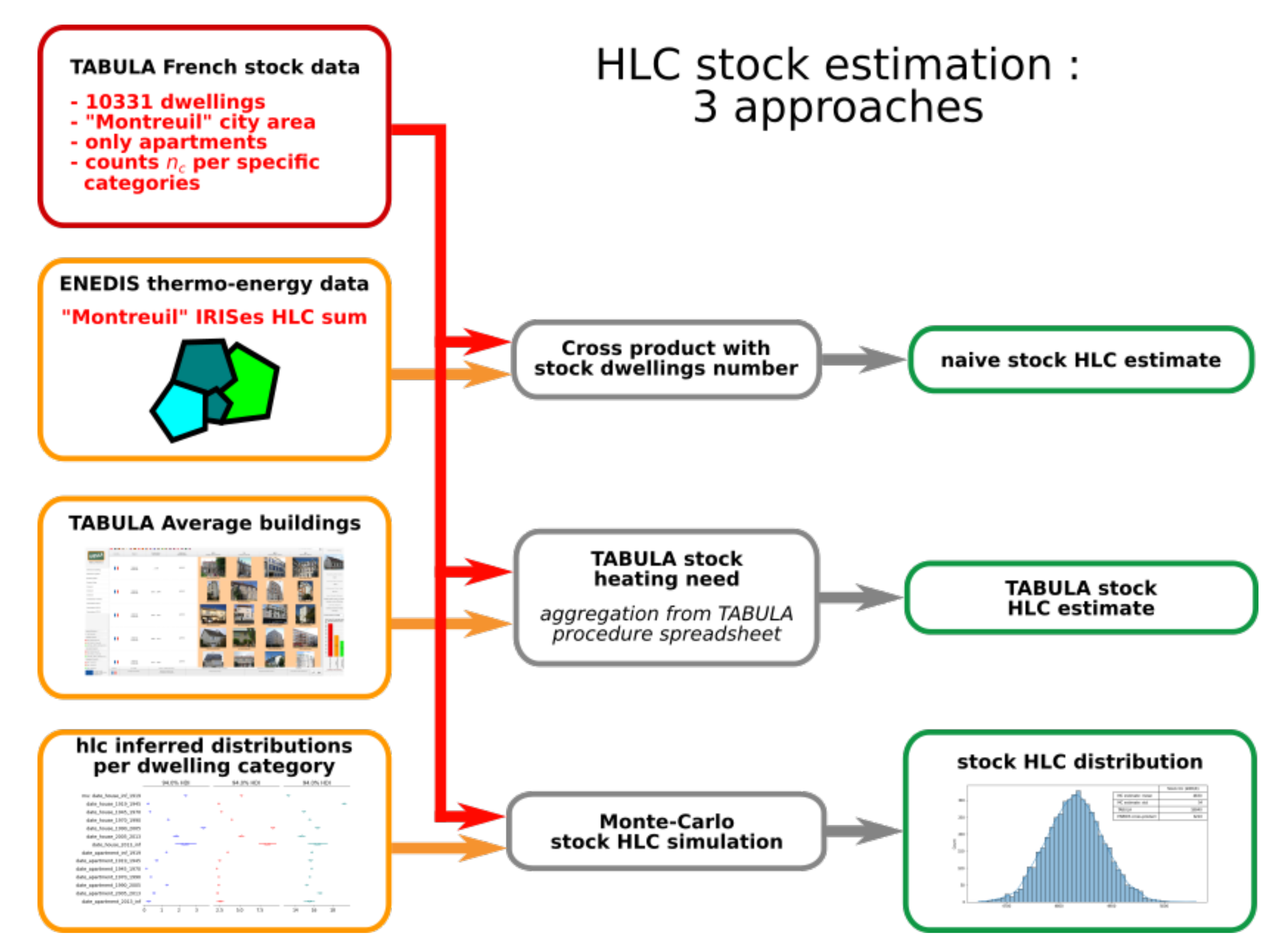
• In a first place, we can naively estimate it from IRIS $\mathit{hlc}$ values in ENEDIS dataset. Under the hypothesis of uniformity of dwelling typologies in the considered area, we sum all IRIS $\mathit{hlc}$ values for the county of Montreuil and resize this sum by the fraction of dwellings in the considered stock (cross-product). The underlying hypothesis is strong, but gives a valuable order of magnitude of 6210 kWh/K.
• Then, we can apply estimations from Building Archetypes and aggregate these estimates for the whole stock. This approach is performed in the TABULA-EPISCOPE French stock study and provides an estimate of net energy needed for heating of 54,353 MWh/year. From this value, we derive the stock $\mathit{hlc}$ by dividing the net heat need by the yearly accumulated difference between internal and external temperature, and get a value of 18,840 kWh/K. This value is computed considering no refurbishment for buildings.
• We can exploit inferred categories distributions for dwellings’ $\mathit{hlc}$ to perform a simple Monte Carlo estimation of the stock $\mathit{hlc}$: Given the rough construction date ranges, we create an interpolated distribution to draw construction dates. For each category of drawn dates, we sample the corresponding number of $\mathit{hlc}$ values from related distributions. Summing-up these $\mathit{hlc}$ values gives an estimate for the whole stock. We repeat the process 5000 times to estimate a representative distribution (Figure 20). The $\mathit{hlc}$ mean result is about 4800 kWh/K, almost 4 times lower than the one from TABULA calculations.

These computations show how inferred distributions for energy signature parameters can be exploited in simple stochastic simulations at district scale. Here, the important difference between TABULA computations and our MC results can be explained by several non-exclusive reasons:

• Physical hypothesis over TABULA archetypes may be biased, and this bias accumulate over the stock. Indeed, we see on Figure 16, Figure 17 and Figure 18 that non-refurbished dwellings have significantly higher values than our inferred ones.
• The ENEDIS dataset may not represent properly the considered stock. However, considered buildings are mostly heated by gas (60%) and electricity [50]. Therefore, if this is the case, errors may come from consumption measurement and estimations.

5. Discussion and Perspectives

In this work, we gather several open data about French dwellings, such as thermo-energetic, weather and census data. This data is aggregated over IRIS areas, i.e., geographic zones representing roughly 500 to 5000 dwellings. By exploiting Bayesian Inference algorithms (NUTS and ADVI) with an appropriate stochastic model, we show it is possible to disaggregate this data and infer parameter uncertainty distributions of the energy signature for each counted dwelling category.

This approach provides the following methodological advantages:

• Since we recover parameter distributions, we have access to confidence intervals.
• We can use parameter distributions in stochastic models to perform Monte Carlo simulations from district to national scale, with uncertainty propagation.
• We perform here data mining while preserving physical sense. This enables critical analysis of resulting parameters, and new insights for energy planning at district or national scale. More generally, the approach can lead to the definition of building archetypes relying on statistical inference rather than parametric assumptions.
• Even if such stochastic models may be complicated to set up and the inference process is computationally intensive, there are no huge limitations in use and applicability. Indeed, on a valid model and dataset, the inference needs to be run only once, and inferred stochastic model can be reused at will in simulations/comparisons with a much lower computing cost. In our case, we use a yearly dataset, so our model can be inferred again once a year as new data is released by providers.

However, in the light of this study, several aspects can be improved:

• In our model, output variables are considered as Gamma random variables. However, one can see in Figure 4 that they are not exactly Gamma distributions since there are some modalities. Indeed, the number of IRIS per dwelling can be only of few hundreds for some of them which reduces the smoothing effect of aggregations. A finer model involving Mixture Gamma distributions (hierarchical combination of Categorical and Gamma distributions) before an aggregating step could help improve the posterior predictive fit. However, such a model may involve much wider tensors and lead to memory and processing power issues (depending on implementation) since it could involve sampling for each dwelling instead of IRISes only.
• Using the provided census data as is, we cannot simply go towards a more detailed inference. One may want to infer the $\mathit{hlc}$ distribution for a specific dwelling type, surface and date range, but census for these joint categories are not in our original dataset. A naive approach would estimate joined ratios by simply multiplying marginal ratios. For example, if for an IRIS the ratio of houses built after 2005 is $0.5$ and the ratio of dwellings with surface between 100 and 120 is also $0.5$, then the ratio of houses built after 2005 and with surface between 100 and 120 would be estimated as $0.25$. However, this approach is only valid for independent variables, which is definitely not the case here. Moreover, some joint categories may have very few appearances in the whole national stock. For all these reasons, our trials with the naive approach failed consistently to converge or give interpretable results. If we want a more detailed model, we need here a better way to estimate all joint categories. This is a quite large and ill-posed problem, often found in literature under the terms of “population disaggregation”. For our case, we have numerous IRISes, therefore one can try to exploit the observed dependency between provided ratios to estimate joint ratios.
• MCMC sampling is computationally intensive and not very scalable: approaches of VI must be explored if one want to explore more detailed models. Since VI is more likely to provide biased results, one may have to define appropriate validation strategies when using this approach.

Besides, other studies could go towards further validation and application of this work:

• In this study, we compared our inference results with average buildings from the TABULA-EPISCOPE projects. This comparison showed similar patterns for $\mathit{hlc}$ values in studied categories. However, TABULA values are generally higher, and with important differences for average buildings without refurbishment. It could be of great interest to pursue similar comparisons with other building archetypes and UBEM tools, such as TEASER or City Energy Analyst. Moreover, such comparisons can be done on a fully instrumented dwellings stock, to compare inferred signatures with the directly computed ones.
• Next studies should also focus on practicability, validation on detailed datasets, use in more complex models than energy signature (dynamic models). Stochastic models used in BI can be hard to set up and parameterize, since convergence is very sensitive to model formulation and parameterization. Hence, there is still large room for improvement towards ease of use in the urban energy planning community.
• The BI approach can also be used on individual dwellings to infer energy signature from annual consumption measures and external temperature. Since we have the distribution of energy signature parameters per dwelling category, one may use them as priors for a specific dwelling to reduce the necessary amount of data for a reliable inference, and have a good estimation of the signature with only few weeks of data instead of at least one year.

References

1. Tavakoli, A.; Saha, S.; Arif, M.T.; Haque, M.E.; Mendis, N.; Oo, A.M.T. Impacts of grid integration of solar PV and electric vehicle on grid stability, power quality and energy economics: A review. IET Energy Syst. Integr. 2020, 2, 243–260. [Google Scholar] [CrossRef]
2. Abergel, T.; Dean, B.; Dulac, J. Towards a Zero-Emission, Efficient, and Resilient Buildings and Construction Sector; Global Status Report; UN Environment and International Energy Agency: Brussels, Belgium, 2017; p. 48. [Google Scholar]
3. Roth, J.; Lim, B.; Jain, R.K.; Grueneich, D. Examining the feasibility of using open data to benchmark building energy usage in cities: A data science and policy perspective. Energy Policy 2020, 139, 111327. [Google Scholar] [CrossRef]
4. Fremouw, M.; Bagaini, A.; De Pascali, P. Energy Potential Mapping: Open Data in Support of Urban Transition Planning. Energies 2020, 13, 1264. [Google Scholar] [CrossRef] [Green Version]
5. Urban Data Platform Plus. 2021. Available online: https://urban.jrc.ec.europa.eu/#/en (accessed on 1 June 2021).
6. Institut Wohnen und Umwelt (IWU). EPISCOPE and TABULA Website. 2016. Available online: https://episcope.eu/welcome/ (accessed on 1 June 2021).
7. TABULA WebTool. 2016. Available online: https://webtool.building-typology.eu/#bm (accessed on 1 June 2021).
8. ENEDIS. Enedis Open Data. 2021. Available online: https://data.enedis.fr/explore/?sort=modified (accessed on 1 June 2021).
9. ADEME. Portail Open Data de l’ADEME. Available online: https://data.ademe.fr (accessed on 1 June 2021).
10. Plateforme Ouverte des Données Publiques Françaises: Environnement, Énergie, Logement. Available online: https://www.data.gouv.fr (accessed on 1 June 2021).
11. Data MetropoleGrenoble: Saisissez vous des Données. Available online: https://data.metropolegrenoble.fr/ (accessed on 1 June 2021).
12. Open data de la Métropole de Lyon. Available online: https://data.grandlyon.com/accueil (accessed on 1 June 2021).
13. Paris Data Platform. Available online: https://opendata.paris.fr/pages/home/ (accessed on 1 June 2021).
14. Hotmaps Project: TheOpen Source Mapping and Planning Tool for Heating and Cooling. Available online: https://www.hotmaps-project.eu/ (accessed on 6 June 2021).
15. Pezzutto, S.; Croce, S.; Zambotti, S.; Kranzl, L.; Novelli, A.; Zambelli, P. Assessment of the Space Heating and Domestic Hot Water Market in Europe - Open Data and Results. Energies 2019, 12, 1760. [Google Scholar] [CrossRef] [Green Version]
16. Planheat Project Website. 2021. Available online: http://planheat.eu/ (accessed on 7 June 2021).
17. Swan, L.G.; Ugursal, V.I. Modeling of end-use energy consumption in the residential sector: A review of modeling techniques. Renew. Sustain. Energy Rev. 2009, 13, 1819–1835. [Google Scholar] [CrossRef]
18. Zhuravchak, R.; Pedrero, R.A.; del Granado, P.C.; Nord, N.; Brattebø, H. Top-down spatially-explicit probabilistic estimation of building energy performance at a scale. Energy Build. 2021, 238, 110786. [Google Scholar] [CrossRef]
19. Kavgic, M.; Mavrogianni, A.; Mumovic, D.; Summerfield, A.; Stevanovic, Z.; Djurovic-Petrovic, M. A review of bottom-up building stock models for energy consumption in the residential sector. Build. Environ. 2010, 45, 1683–1697. [Google Scholar] [CrossRef]
20. Ferrando, M.; Causone, F.; Hong, T.; Chen, Y. Urban building energy modeling (UBEM) tools: A state-of-the-art review of bottom-up physics-based approaches. Sustain. Cities Soc. 2020, 62, 102408. [Google Scholar] [CrossRef]
21. Fonseca, J.A.; Nguyen, T.A.; Schlueter, A.; Marechal, F. City Energy Analyst (CEA): Integrated framework for analysis and optimization of building energy systems in neighborhoods and city districts. Energy Build. 2016, 113, 202–226. [Google Scholar] [CrossRef]
22. Remmen, P.; Lauster, M.; Mans, M.; Fuchs, M.; Osterhage, T.; Müller, D. TEASER: An open tool for urban energy modelling of building stocks. J. Build. Perform. Simul. 2018, 11, 84–98. [Google Scholar] [CrossRef]
23. Hong, T.; Chen, Y.; Lee, S.H.; Piette, M. CityBES: A Web-based Platform to Support City-Scale Building Energy Efficiency. Urban Comput. 2016, 14. [Google Scholar] [CrossRef]
24. Robinson, D.; Haldi, F.; Leroux, P.; Perez, D.; Rasheed, A.; Wilke, U. CitySim: Comprehensive micro-simulation of resource flows for sustainable urban planning. In Proceedings of the Eleventh International IBPSA Conference, Glasgow, Scotland, 27–30 July 2009; pp. 1083–1090. [Google Scholar]
25. Pajot, C.; Artiges, N.; Delinchant, B.; Rouchier, S.; Wurtz, F.; Maréchal, Y. An Approach to Study District Thermal Flexibility Using Generative Modeling from Existing Data. Energies 2019, 12, 3632. [Google Scholar] [CrossRef] [Green Version]
26. Kotzur, L. Future Grid Load of the Residential Building Sector. Ph.D. Thesis, RWTH Aachen University, Aachen, Germany, 2018. [Google Scholar]
27. Lim, H.; Zhai, Z.J. Review on stochastic modeling methods for building stock energy prediction. Build. Simul. 2017, 10, 607–624. [Google Scholar] [CrossRef] [Green Version]
28. Pasichnyi, O.; Wallin, J.; Kordas, O. Data-driven building archetypes for urban building energy modelling. Energy 2019, 181, 360–377. [Google Scholar] [CrossRef]
29. Cerezo, C.; Sokol, J.; AlKhaled, S.; Reinhart, C.; Al-Mumin, A.; Hajiah, A. Comparison of four building archetype characterization methods in urban building energy modeling (UBEM): A residential case study in Kuwait City. Energy Build. 2017, 154, 321–334. [Google Scholar] [CrossRef]
30. Wang, C.K. Urban Building Energy Modeling Using a 3D City Model and Minimizing Uncertainty through Bayesian Inference: A Case Study Focuses on Amsterdam Residential Heating Demand Simulation. Master’s Thesis, Delft University of Technology, Delft, The Netherlands, 2018. [Google Scholar]
31. Sokol, J.; Cerezo Davila, C.; Reinhart, C.F. Validation of a Bayesian-based method for defining residential archetypes in urban building energy models. Energy Build. 2017, 134, 11–24. [Google Scholar] [CrossRef]
32. ENEDIS. Consommation et Thermosensibilité Electriques par Secteur d’Activité à la Maille IRIS. 2017. Available online: https://data.enedis.fr/explore/dataset/consommation-electrique-par-secteur-dactivite-iris/information/?refine.annee=2017 (accessed on 27 May 2021).
33. INSEE. Logement en 2016|Insee. 2016. Available online: https://www.insee.fr/fr/statistiques/4228432. (accessed on 27 May 2021).
34. IGN. Géoservices|Accéder Au Téléchargement des Données Libres IGN. 2017. Available online: https://geoservices.ign.fr/documentation/diffusion/telechargement-donnees-libres.html#contoursiris. (accessed on 27 May 2021).
35. Météo-France. Données Publiques de Météo-France: Données SYNOP Essentielles OMM. 2017. Available online: https://donneespubliques.meteofrance.fr/?fond=produit&id_produit=90&id_rubrique=32. (accessed on 27 May 2021).
36. Chib, S.; Greenberg, E. Understanding the Metropolis-Hastings Algorithm. Am. Stat. 1995, 49, 327–335. [Google Scholar] [CrossRef] [Green Version]
37. Betancourt, M. A Conceptual Introduction to Hamiltonian Monte Carlo. arXiv 2018, arXiv:1701.02434. [Google Scholar]
38. Hoffman, M.D.; Gelman, A. The No-U-Turn sampler: Adaptively setting path lengths in Hamiltonian Monte Carlo. J. Mach. Learn. Res. 2014, 15, 1593–1623. [Google Scholar]
39. Kucukelbir, A.; Tran, D.; Ranganath, R.; Gelman, A.; Blei, D.M. Automatic Differentiation Variational Inference. arXiv 2016, arXiv:1603.00788. [Google Scholar]
40. Lee, D.; Carpenter, B.; Li, P.; Morris, M.; Betancourt, M.; Maverickg, M.; Brubaker, M.; Trangucci, R.; Inacio, M.; Kucukelbir, A.; et al. Stan software: V2.17.1. Zenodo 2017. [Google Scholar] [CrossRef]
41. Bingham, E.; Chen, J.P.; Jankowiak, M.; Obermeyer, F.; Pradhan, N.; Karaletsos, T.; Singh, R.; Szerlip, P.; Horsfall, P.; Goodman, N.D. Pyro: Deep Universal Probabilistic Programming. J. Mach. Learn. Res. 2019, 20, 1–6. [Google Scholar]
42. Salvatier, J.; Wiecki, T.V.; Fonnesbeck, C. Probabilistic programming in Python using PyMC3. PeerJ Comput. Sci. 2016, 2, e55. [Google Scholar] [CrossRef] [Green Version]
43. Salvatier, J.; Wiecki, T.; Patil, A.; Kochurov, M.; Engels, B.; Lao, J.; Colin; Martin, O.; Seyboldt, A.; Rochford, A.; et al. PyMC3 software: V3.11.2. Zenodo 2021. [Google Scholar] [CrossRef]
44. Davidson-Pilon, C. Bayesian Methods for Hackers: Probabilistic Programming and Bayesian Inference; Addison-Wesley: New York, NY, USA, 2016. [Google Scholar]
45. Artiges, N.; Rouchier, S.; Delinchant, B. Bayesian Archetypes: Energy Signature Inference from National Data for Statistical Definition of Buildings Archetypes. 2021. Available online: https://gricad-gitlab.univ-grenoble-alpes.fr/districtmodeling/bayesian_archetypes (accessed on 1 September 2021). [CrossRef]
46. Kumar, R.; Carroll, C.; Hartikainen, A.; Martin, O. ArviZ a unified library for exploratory analysis of Bayesian models in Python. J. Open Source Softw. 2019, 4, 1143. [Google Scholar] [CrossRef]
47. Gelman, A.; Rubin, D.B. Inference from Iterative Simulation Using Multiple Sequences. Stat. Sci. 1992, 7, 457–472. [Google Scholar] [CrossRef]
48. Geyer, C.J. Introduction to Markov Chain Monte Carlo. In Handbook of Markov Chain Monte Carlo; Chapman and Hall/CRC: London, UK, 2011. [Google Scholar]
49. Vehtari, A.; Gelman, A.; Simpson, D.; Carpenter, B.; Bürkner, P.C. Rank-normalization, folding, and localization: An improved R for assessing convergence of MCMC. Bayesian Anal. 2021, 1, 1–28. [Google Scholar] [CrossRef]
50. Pouget Consultants. National Report on Pilot Actions. Technical Report Deliverable D3.1. 2015. Available online: https://episcope.eu/fileadmin/episcope/public/docs/pilot_actions/FR_EPISCOPE_LocalCaseStudy_Pouget.pdf (accessed on 9 July 2021).
51. TABULA Episcope Project. Average Buildings: Energy Need for Heating (French Case). Available online: https://s2.building-typology.eu/abpdf/FR_L_01_EPISCOPE_CaseStudy_TABULA_Local.pdf (accessed on 9 July 2021).
Figure 1. Main approaches in Urban Building Energy Modeling (UBEM).
Energies 14 05651 g001
Figure 2. The energy signature method.
Energies 14 05651 g002
Figure 3. Geographical disposition of used IRIS and related 2017 values for (a) apartments ratio per IRIS (b) average hlc per dwelling (c) average base consumption per dwelling, and (d) computed T s per IRIS. White areas are for missing data.
Energies 14 05651 g003
Figure 4. Aggregated distributions of main variables at national scale.
Energies 14 05651 g004
Figure 5. Census data for each recorded dwelling category.
Energies 14 05651 g005
Figure 6. Inference model graph for INSEE dwelling categories. × represents the product of dimensions.
Energies 14 05651 g006
Figure 7. Posterior traceplot for houses and apartments model. Left part shows distributions of samples (samples values on x-axis and density on y) and right part their values across the sampling process (samples number on x-axis and values on y). For each parameter ( μ , and σ ), each color matches an element of the corresponding tensor (elements for hlc , base consumption and T s for each category). For each color, we plot a curve per sampling chain (4 in this case). All inferred variables sample values are displayed here regardless of their units.
Energies 14 05651 g007
Figure 8. Posterior predictive distributions for training and validation data—apartments and houses model.
Energies 14 05651 g008
Figure 9. Inference results for houses and apartments model with 94 % HDI (Highest Density Interval). Central points are for mean values and bold lines for inter-quartiles.
Energies 14 05651 g009
Figure 10. Posterior trace for surfaces model.
Energies 14 05651 g010
Figure 11. Posterior predictive distributions for training and validation data—surfaces model.
Energies 14 05651 g011
Figure 12. Inference results for surfaces model.
Energies 14 05651 g012
Figure 13. Posterior trace for types and dates model.
Energies 14 05651 g013
Figure 14. Posterior predictive distributions for training and validation data—types and dates model.
Energies 14 05651 g014
Figure 15. Inference results for types and dates model.
Energies 14 05651 g015
Figure 16. hlc comparisons between TABULA average buildings and inferred values (dwelling types model).
Energies 14 05651 g016
Figure 17. hlc comparisons between TABULA average buildings and inferred values (surfaces model).
Energies 14 05651 g017
Figure 18. hlc comparisons between TABULA average buildings and inferred values (types and dates model).
Energies 14 05651 g018
Figure 19. Stock hlc estimation techniques.
Energies 14 05651 g019
Figure 20. Monte-Carlo simulation for TABULA french stock.
Energies 14 05651 g020