Abstract
The aim of this study was to develop trajectory planning that would allow an autonomous racing car to be driven as close as possible to what a driver would do, defining the most appropriate inputs for the current scenario. The search for the optimal trajectory in terms of lap time reduction involves the modeling of all the non-linearities of the vehicle dynamics with the disadvantage of being a time-consuming problem and not being able to be implemented in real-time. However, to improve the vehicle performances, the trajectory needs to be optimized online with the knowledge of the actual vehicle dynamics and path conditions. Therefore, this study involved the development of an architecture that allows an autonomous racing car to have an optimal online trajectory planning and path tracking ensuring professional driver performances. The real-time trajectory optimization can also ensure a possible future implementation in the urban area where obstacles and dynamic scenarios could be faced. It was chosen to implement a local trajectory planning based on the Model Predictive Control (MPC) logic and solved as Linear Programming (LP) by Sequential Convex Programming (SCP). The idea was to achieve a computational cost, 0.1 s, using a point mass vehicle model constrained by experimental definition and approximation of the car’s GG-V, and developing an optimum model-based path tracking to define the driver model that allows A car to follow the trajectory defined by the planner ensuring a signal input every 0.001 s. To validate the algorithm, two types of tests were carried out: a Matlab-Simulink, Vi-Grade co-simulation test, comparing the proposed algorithm with the performance of an offline motion planning, and a real-time simulator test, comparing the proposed algorithm with the performance of a professional driver. The results obtained showed that the computational cost of the optimization algorithm developed is below the limit of 0.1 s, and the architecture showed a reduction of the lap time of about 1 s compared to the offline optimizer and reproducibility of the performance obtained by the driver.
1. Introduction
In recent years, research on the automotive field has focused on making cars more and more able to make decisions autonomously due to the growth of electric and electronic technologies on modern road cars and to the possibility of providing increased safety and improved performance.
In the racing world, where the scenario is static and known, the perception system has a simple implementation, and good results have already been achieved, as shown, for example, in [1].
The main challenge is to improve performance through the use of models that represent the dynamics of the vehicle as faithfully as possible while ensuring an acceptable computational effort for real-time implementation.
The aim of this paper was to develop a trajectory planner able to update the trajectory online with the car progress on the track, trying to replicate the capabilities of a human driver. Then, the trajectory planning was embedded with a path tracking consisting of a Linear Quadratic Regulator (LQR) that provides the car’s input signals: steering wheel angle, accelerator and brake pedals signals.
In this way, even if in a racing world scenario, real-time trajectory optimization can ensure a possible future implementation in the urban area where obstacles and dynamic scenarios could be faced.
To ensure a trajectory tracking able to reduce the lap time, the state-of-the-art offers different approaches both from the architecture and methodology point of view. From the architecture point of view, the research is divided between the ones that used a real-time single algorithm to plan and track the trajectory [2,3], others that preferred to separate the planner from the tracker by having the first offline and the second work in real-time [4], and others that divided trajectory planning and tracking but implemented them both in real-time [5,6,7]. The first architecture type, as said in [8], gives the advantage of incorporating tire force constraints in a straight-forward way. However, the integration of trajectory planning and tracking approaches can work for autonomous RC-cars but is difficult to scale to complex scenarios due to the non-convex nature of the constraints imposed by multiple vehicles. In addition, it implies a more complex tuning. Instead, there are many studies about the offline trajectory planner with good performances in terms of lap time reduction and car set-up, allowing to implement a vehicle model with more Degrees of Freedom (DoF) [9], adding also a friction coefficient mapping [4] and involving different methodologies. Some authors preferred to develop a geometrical solution by minimizing the curvature [8] or generating a racing line using professional driving techniques [10]. However, these techniques do not provide information about vehicle dynamics, despite the fact that the trajectory of least curvature ensures lap similar to the trajectory optimization techniques [8]. Therefore, other researchers preferred to face the problem as a kinodynamic problem by finding the optimal trajectory, minimizing the lap time and considering both the kinematic constraints of the track and the dynamic constraints of the vehicle [4,11]. Facing the problem from the kinodynamic point of view considers that the non-convexity of the trajectory does not allow a global solution [8,10] but a local one [12,13,14] using Sequential Convex Programming (SCP) methodology [7].
The study presented in this paper has involved the development of a trajectory planner that every 0.1 s provides the speed and trajectory that the car follows thanks to an implemented path tracking that controls the car motion every 0.001 s. The real-time implementation of both trajectory planning and path tracking is advantageous in terms of performance and safety. In fact, during the race, a professional driver is able to feel the car conditions and choose the trajectory that ensures the best performance. In the same way, a trajectory planner must provide the fastest trajectory for the dynamic and scenario conditions in which the vehicle is located. In [7], it was decided to use a point mass vehicle model and implement a Model Predictive Control (MPC) with the SCP approach. To simplify the algorithm without incurring in infeasibility and further reduce the computational time, it was chosen to solve the Linear Programming (LP) problem instead of the Quadratic Programming (QP) problem and to reduce the losses due to linearization, it was chosen to represent the car’s GG-V with conical constraint equations. Furthermore, the weights and variables of optimization change with the track sequences, allowing the designer to change the constraints with changes in scenario and vehicle dynamics.
In Section 2, the architecture developed is shown. Then, in Section 3, the trajectory planner model and methodologies are explained with the hypothesis and the reference system used, followed by Section 4 where the path tracking developed is shown. In the last section, the tests performed will provide the results obtained by the algorithm in terms of the car’s trajectory and lap time, comparing them with those obtained by the CarRealTime (CRT) MaxPerformance event, and by a professional driver in a real-time car simulator.
2. Trajectory Tracking Architecture
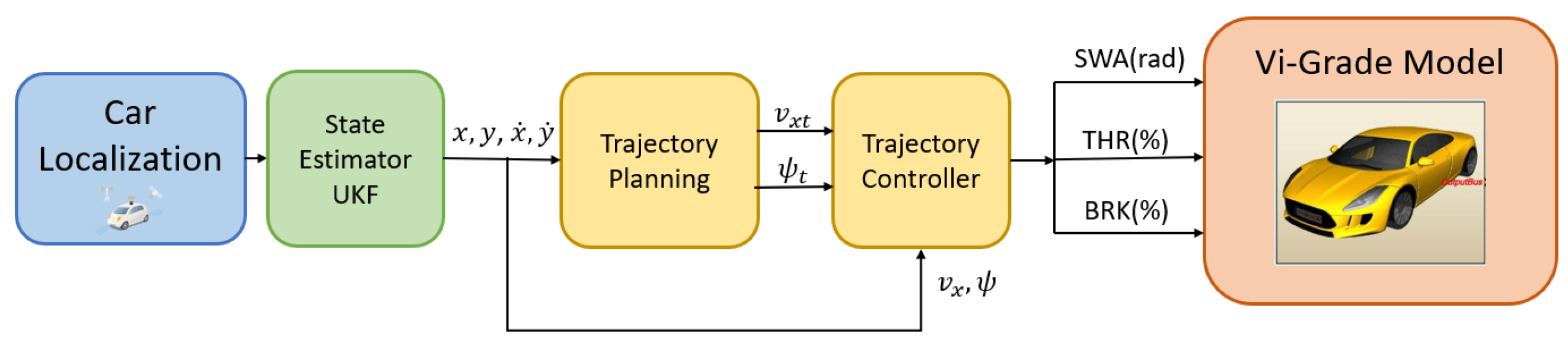
In Figure 1, the architecture developed is shown. The idea is to divide the trajectory planning from the path tracking instead of implemented a single with a complex and detailed vehicle and tire model by ensuring a real-time implementation of the algorithm that the current technologies do not allow otherwise. Thus, an optimizer is implemented as trajectory planning, giving the reference position and speed to minimize the lap time every 0.1 s, and an optimum controller is implemented to allow the car to follow reference state values by defining the input steering wheel angle, throttle pedal and braking pedal every 0.001 s. These sample time values were necessary because an increase compared to the time of 0.1 s in providing the position and speeds that the vehicle must have is excessive compared to the speed of the vehicle resulting in a delay with respect to its position; from the tests undertaken, an increase in the time of 0.001 s of the controller was found to worsen the performance of the control.
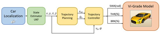
Figure 1.
System architecture.
The trajectory planning and path tracking use the states of the car in the race track as feed-back. These states are estimated by a Localization Layer composed of an Unscented Kalman Filter (UKF) that uses the sensors measurements shown in Table 1.

Table 1.
Variables measured by sensors.
All the layers shown in Figure 1 were implemented in Matlab-Simulink software and then compiled in C to be used in the real-time car simulator of Vi-Grade. The different control algorithms were integrated into the same Simulink model considering the rate transition between subsystem with different sample times. Since the difference in time step implies that the optimization layer provides the same value for 100 steps of the controller, an integration algorithm between the path planning and trajectory controller is developed. This algorithm ensures that the positions and velocities provided by the optimizer to the controller increase with the constant acceleration optimized, and after 100 steps, the vehicle achieves the position and velocity values expected by the optimizer. In the event that the vehicle fails to be in the expected condition, the change of values given by the change of optimizer steps needs to be compatible with the vehicle’s possible acceleration limits based on the state the vehicle is in. The logic is shown in Equation (1):
where are the speeds and positions that the car has to follow in the current time; are the speeds and positions that the car had at the previous time step of the controller; are, respectively, the controller sample time of 0.001 s, and the difference between the actual and previous time of the optimizer in the sample time of the controller; 0.1 is a tuning value that reduced the speed step between the actual and the future value if it is higher than 0.5 m/s.
3. Trajectory Planning
To set-up the MPC optimization problems, the Gurobi solver is used, a commercial solver with parallel algorithms for large-scale linear programs, quadratic programs, and mixed integer programs. From the Gurobi optimization reference manual [15], the problem was implemented in the following form:
where the Objective Function (2), the Vehicle Model (3), the constraints used to represent the vehicle dynamic and track limitation (4), and the Bound Constraints (5) are shown and will be explained in the following subsections.
The problem is faced as an LP optimization, and its solutions are found by iterating the optimization every time step: the positions, , velocities, , and accelerations, , are the state values optimized at the previous step; so the current iteration defines the optimum state, , and input, for all the prediction horizon lengths. The variables weights of the Objective Function, − − − , are defined by a tuning process, and the prediction horizon was chosen to be composed of 120 time steps to ensure that the optimizer should be able to see the following curve when the longest straight begins, as tests have shown that the performance was satisfactory.
3.1. Models
To ensure a computational cost of 0.1 s, the vehicle was modeled as a point mass model, with the following assumption:
- The vehicle’s side-slip and tires’ slip angles are negligible. This means that the velocity vector is always tangent to the trajectory and it allows to ignore behavior such as drifting, spinning, or sliding;
- The tires’ slippage is negligible;
- The longitudinal and lateral weight transfers are neglected in the vehicle model but will be considered in the constraint formulations;
- The racetrack is flat.
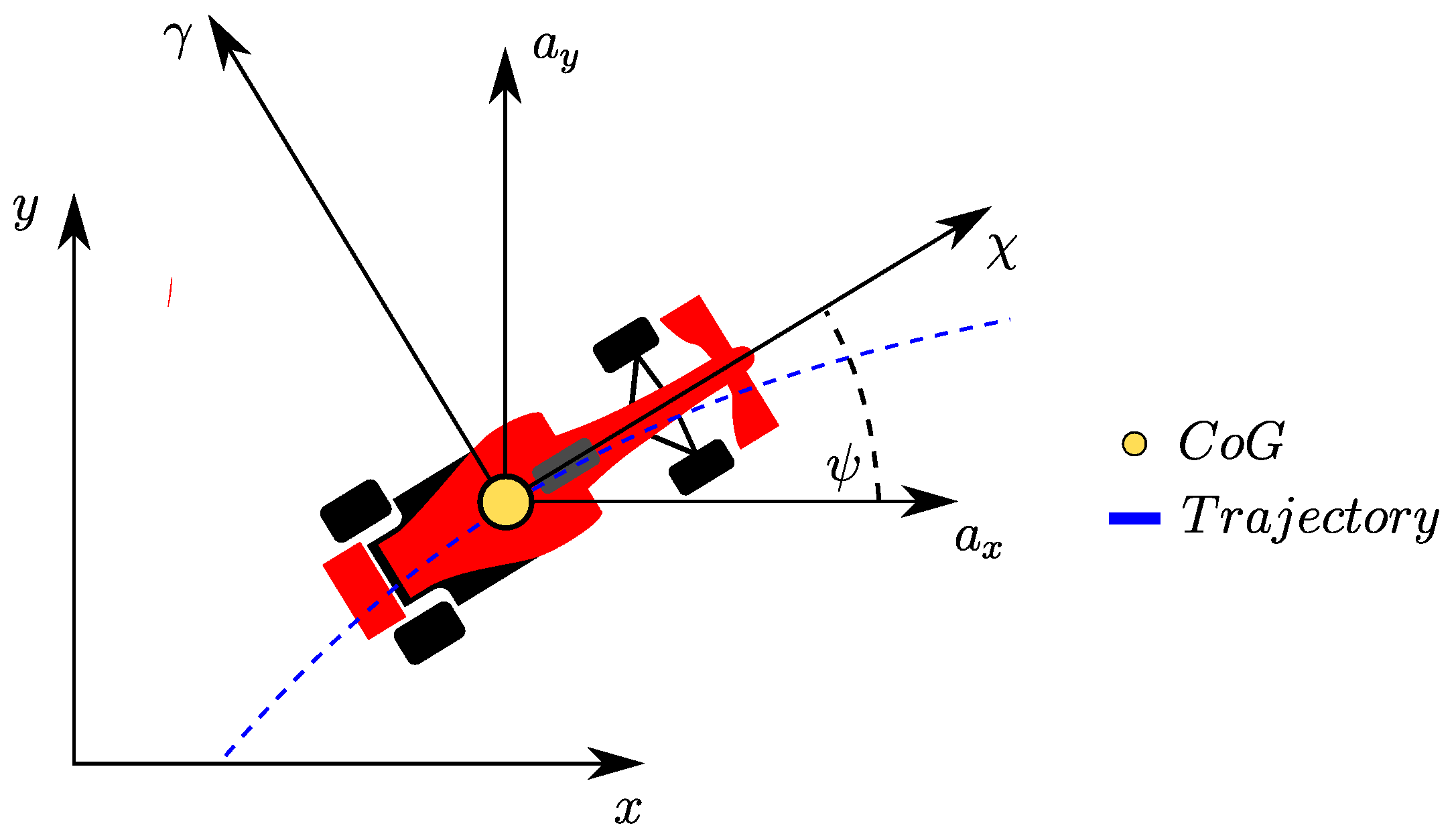
Therefore, referring to the coordinate system shown in Figure 2: x,y are the global coordinate system when stationary with respect to the racetrack; , are the vehicle coordinate system; and is the vehicle yaw angle that indicates the tangent to the trajectory. The dynamic model was implemented in the discrete state space Equation (6) and detailed by Equation (7).
where, in this case, i indicates the time-step index; is the state vector composed by the vehicle position and velocity vector in the global coordinate system, and ; is the input vector composed by the vehicle acceleration vector in global coordinate system, ; is the system matrix and is the input matrix made explicit in Equation (7). From these equations, it is possible to deduce that to have a linear system, the time-step, , must chose constant. Thus, the prediction horizon is discretized with constant time intervals, and the discrete model, shown in Equation (3), is then iterated forward in time from a time-step to the subsequent one.

Figure 2.
Global and vehicle coordinate systems.
3.2. Objective Function
The Objective Function proposed in this work is purely linear, as shown in Equation (2). This is a benefit because it reduces the optimization time and allows one to not worry about defining a positive objective matrix to ensure a feasible solution. It is composed of two strategies:
- Minimizing time strategy;
- Slack variables.
The first strategy aims to minimize the lap time, and the second one allows softening the hard limit of the constraints.
3.2.1. Minimizing Time Strategy
Since a constant discretization time of the prediction horizon is chosen to make Equation (7) linear, maximizing the distance traveled in the direction of the tangent vector of the mid-line could be a strategy to cover the largest number of racetrack sectors. This strategy was expressed within the objective function as follows:
where it maximized the longitudinal and lateral distance between the current, , and previous, , position points projected in the tangent direction, , for all the points of the prediction horizon .
3.2.2. Slack Variables
To avoid the infeasible problem, the slack variable strategy is used [16]. This methodology ensures avoiding that the constraints equations are not strictly equal to a constant limit but to an enlarged or reduced one by adding to the constraint a positive variable, weighted in the objective function. In this way, the designer can strengthen or relax the constraints by increasing or decreasing the associated weights.
In Equation (9), , , and are the slack variables and , , , are the weights, respectively. In this work, by associating the weights to the nodes of the mid-line, , it is possible to impose to the solver not only the ability to vary the constraints but also to decide whether one point of the racetrack is more important than another in terms of limit variations available, as a human driver can do.
3.3. Linear and Quadratic Constraints
To ensure optimized solutions compatible with vehicle dynamics and track limits, the vehicle accelerations and positions are limited by constraint Equations (4), which can be divided into three categories:
3.3.1. Racetrack Limitations
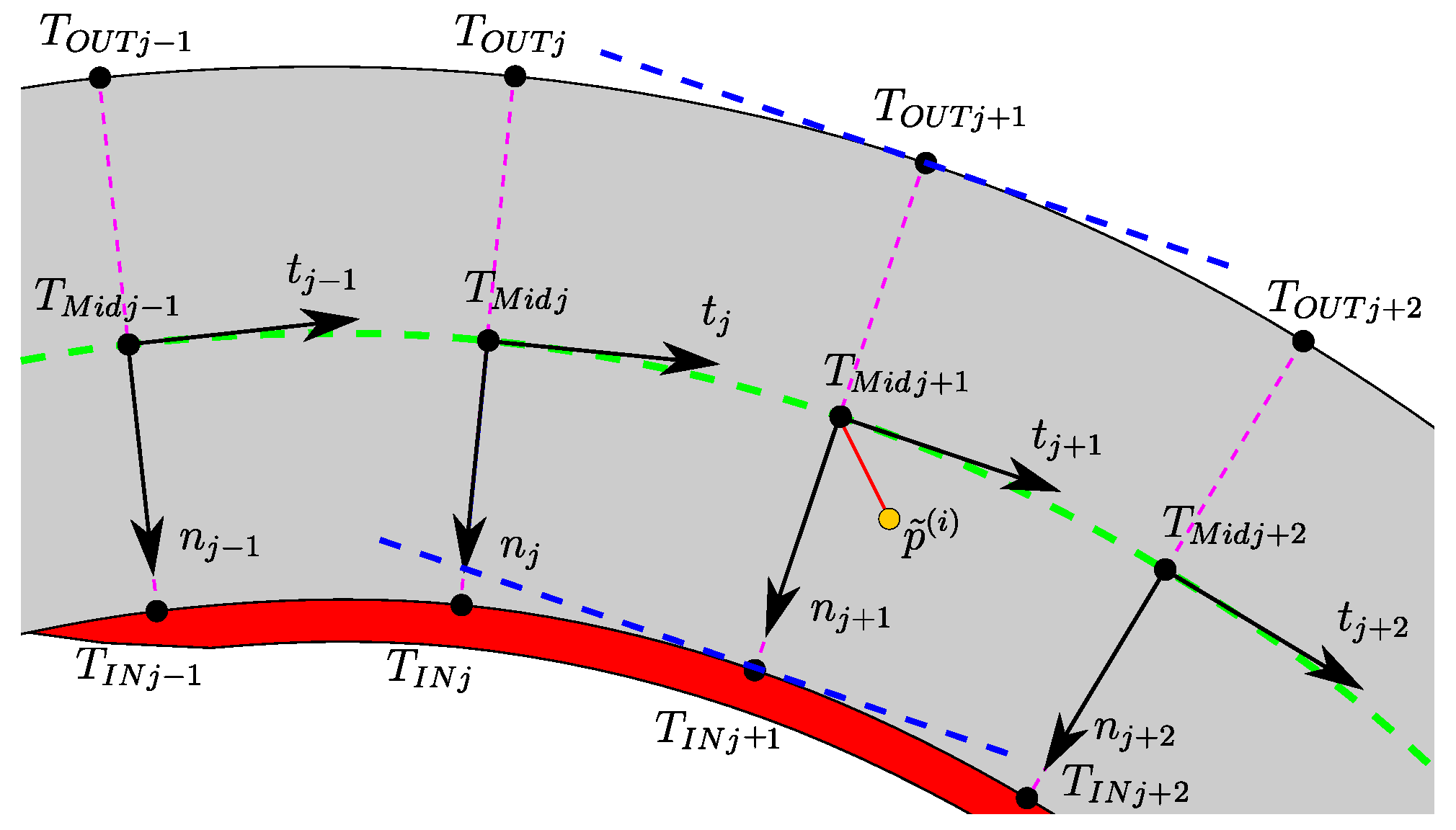
In order to constrain the optimizer to provide output car positions within the path area, the optimization was solved by using the SCP approach as [17] suggested. Thus, the constraint is not the entire racetrack area, which involves a non-convex problem, but smaller racetrack sections where the problem is convex and so solvable. Therefore, it was decided to sample the middle line with points 1 m apart, , and to make these correspond to those intercepted on the inner and outer edge by the normal vector to the middle line and named, respectively, with and in Figure 3. Then, it was possible to constrain the output states of the solver, , within the path area, using the following equations:
where is the position state vector found by the optimization in the current optimization step; and are the limits given by the outer and inner edge referred to the solution found in the previous iteration step, ; is the normal direction to the mid-line, which allows the distance between the two points to be projected in the normal direction; and is the slack variable, which, being constrained in the Bound Constraints Equation (5g) as positive, forces the position of the vehicle to be less than zero making the racetrack constraints more or less rigid depending on the weight assigned to it in the Objective Function (2). Therefore, it is possible to vary the weight of the slack variable in a differentiated way according to the position of the car in the track, being able, for example, to soften it in the presence of a curb by allowing the car to go out of the limits of the track where possible to improve performance.
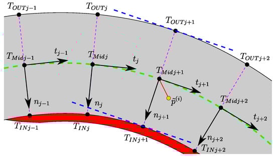
Figure 3.
Representation of the racetrack linear approximation.
3.3.2. GG Limitations
In order to represent the exchange of forces occurring at the point of contact between wheel and road, it was decided to not implement a tire model but to bound the car’s acceleration inside the GG diagram, measured at the center of gravity under steady-state conditions, such as [7,18,19].
The papers [20,21,22] show that the acceleration constraints area has the shape of two semi-ellipses: one stands for the forward acceleration, shown by the blue line in Figure 4a, and the other stands for backward acceleration, shown by the red line in Figure 4a.
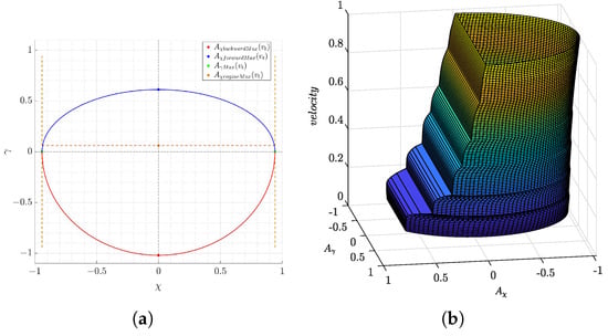
Figure 4.
Single GG diagram of the vehicle and its change with the vehicle speed. (a) Approximation method for the g-g diagram: two half ellipses for tire limits and a line for engine limit. (b) Autonomous driving car GG-V diagram, evaluated through simulation tests.
Empirically defining the maximum acceleration values, , and , the semi-axes of the ellipses are defined and so, the tire, aerodynamic and vehicle system limits are taken into account. Therefore, if the blue and red lines in Figure 4a show the limits just mentioned, the horizontal orange line shows the maximum performance that the car’s engine can achieve in forward acceleration. In addition, these limits change with the vehicle speed because of the drag and engine influence [23,24]; thus, in Figure 4b, different GG diagrams were implemented in the function of the car speed obtaining the car GG-V diagram.
However, to better represent the vehicle dynamic and improve the performance, the idea was to implement the GG-V as quadratic constrains and not linearize its curves as is usually done, while maintaining the sample time under the specification of 0.1 s. However, due to the ability of the LP to handle only one convex quadratic constraint for each variable, a mixed approach was implemented: a conical constraint to reproduce the bigger, lower region associated with the vehicle braking capabilities exactly, and linear constraints to approximate the upper region, which is associated with the vehicle forward acceleration capabilities, being tested empirically, resulting in this region being well-described by the three orange dotted lines shown in Figure 4a. Therefore, the lower GG constraints are implemented as a negative semi-ellipse with the semi-axes values equal to the car’s maximum deceleration. This inequality constraint is shown in the vehicle coordinate system by Equation (11) and in the global coordinate system by Equation (12).
Instead, the upper GG constraints are represented as a set of lines tangent at the positive semi-ellipse. These lines are calculated by finding the tangents at the ellipse in points described by different angles, , thanks to Equation (13) in the coordinate vehicle system and Equation (14) in the global coordinates system.
In all the equations shown, the ratio between the longitudinal speed component, , and speed vector, , is the cosine of the yaw angle ; and the ratio between the lateral speed component, , and speed vector, , is the sine of the yaw angle . Both of these ratios are used to rotate the input vector in the global coordinate system and group the constraints in Equation (4b).
The variable c is a scalar coefficient that can expand or narrow the boundary of the GG diagram and change the tire performances representing degraded contact conditions due, for example, to rain or tire wear. c could be scaled in a global manner for all of the track or could be varied online in local sections being related to the position of the vehicle on the racetrack.
3.3.3. Jerk Limitations
Since the vehicle is modeled as a point mass, sudden variations in acceleration, , can lead to the generation of an angular trajectory that does not represent a real trajectory of a racing car, which actually tends to be smooth. Usually, to avoid this problem, the quadratic variation of the accelerations is implemented as a term of the Objective Function to minimize it. In this study, to maintain the Objective Function as linear, the Jerk Limitations are implemented as constraint equations that require the jerks to be equal to positive slack variables. Therefore, the slack variables are inserted in the cost function as a linear term and a certain weight is assigned to them according to the point on the track where the car is located. In this way, the optimizer is able to determine the accelerations variation necessary to increase performance and maintain a smooth trajectory, and the designer can choose which direction of acceleration to favor in relation to where the car is located on the track, e.g., in a straight line the lateral acceleration can be forced to vary more slowly, favoring a faster variation of the longitudinal accelerations.
In Equation (4c), the strategy is shown, where , are the slack variables used to soften the zero hard limit given to the input vector variation, , rotated in the global coordinate system by . In addition, it was chosen to implement different slack variables for different acceleration vectors diversifying the jerk of the various dynamic system: for forward longitudinal acceleration, for backward longitudinal acceleration, and for lateral acceleration.
3.4. Bound Constraints
As usual, the optimization variables must be limited to effectively guide the solver in the optimization phases. This allows a faster search for the correct solution and reduces the possibility of facing the infeasible problem that results in a reduction in the optimization time. For this reason, the following trust regions were added to the solver: Equation (5a,b), which limit the positions; Equation (5c,d), which limit the speeds; Equation (5e,f), which limit the accelerations; and Equation (5g), which imposes a slack variable that is greater than zero.
4. Path Tracking
Regarding the path tracking, an optimum control was chosen to be implemented by decoupling the longitudinal and lateral vehicle dynamics and ensuring a low computational cost. The developed LQR has a sample time of 0.001 s to define the car input with a certain continuity as a driver will do. In this way, the path planning is embedded with a path tracking to compose the trajectory tracking with a dynamic vehicle model and a reduced time step.
4.1. Vehicle Model
To ensure a linear model to the LQR, the longitudinal and lateral vehicle dynamic are decoupled and modeled separately, obtaining a model where the longitudinal part defines the inputs pedals throttle and brake percentage, and the lateral part defines the steering wheel angle signal input.
4.1.1. Longitudinal Model
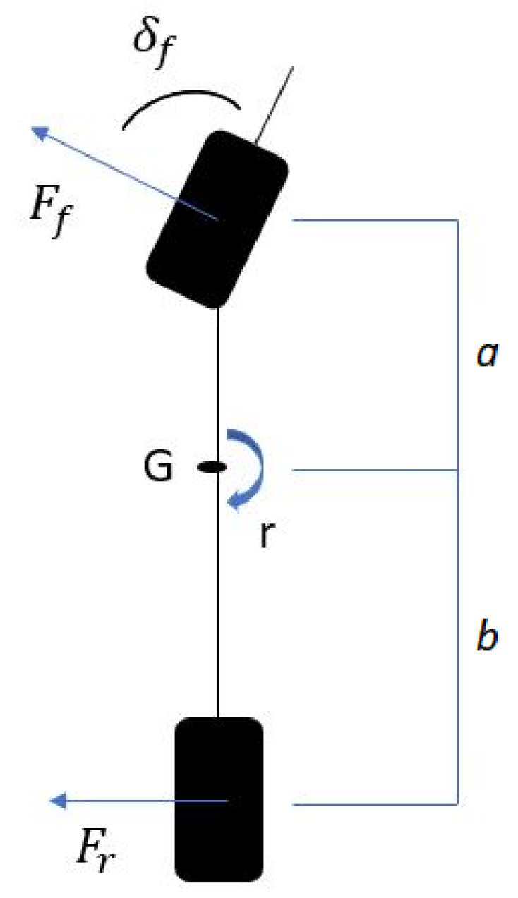
About the longitudinal model, it is supposed to have the single track vehicle model, shown in Figure 5, in which the longitudinal acceleration of the vehicle is set equal to the sum of the longitudinal tire forces:
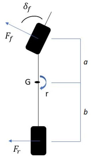
Figure 5.
Single track vehicle model.
Considering the total longitudinal force that the car has to have as a percentage of the maximum tracking force that the engine and braking system can express, the longitudinal vehicle model could be implemented as:
where is the vehicle longitudinal acceleration; C is the throttle or brake pedal percentage in the range [0–100](%); is the maximum force that the engine and brake system can give; and m is the vehicle mass.
4.1.2. Lateral Model
Regarding the lateral model, the single track vehicle model shown in Figure 5 was used, considering the lateral and yaw dynamic balance given by [19], as follows:
where v and r are, respectively, the lateral speed component and yaw rate; and are the cornering stiffness tire parameters; u is the longitudinal speed component; a and b are, respectively, the front and rear wheelbase of the vehicle; m, J and R are the mass, vertical moment of inertia and wheel radius of the car.
4.2. LQR
Considering the longitudinal and lateral vehicle dynamics shown in the previous subsection, a LQR can be implemented by tracking the longitudinal and lateral vehicle speed and position found by the trajectory planning. In fact, the optimized longitudinal vehicle speed can be considered as the target speed that the vehicle has to have and subtracted from the actual longitudinal vehicle speed obtaining:
where and m are constant variable and is the throttle pedal percentage if the speed error, , is positive and the brake pedal percentage if it is negative, saturated from 0 to 100%.
Instead, to follow the lateral dynamics suggested by the path planning, the yaw and lateral vehicle position and speed are tracked, considering the errors between the actual vehicle values and the reference values exiting the trajectory planning. Thus, replacing the Equations (17) and (18) in (21) and considering the longitudinal vehicle speed, u, as a constant variable, the following was obtained:
Therefore, the dynamic state space has the following representation:
where the errors of longitudinal, lateral and yaw position and rate are the states, , which must be minimized by defining the car input as follows:
Here, K is the gains matrix calculated by solving the following offline optimization:
where the state and the input vectors are appropriately weighted by the matrices Q and R.
However, the state space formulation shown in Equation (25) does not ensure that the tracking errors converge to zero, even though the matrix is asymptotically stable [25]. This is due to the omission of the term steady state:
To ensure zero steady state errors, a feed-forward term is added to the state feed-back assuming that the steering controller is obtained by state feed-back plus a feed-forward term:
where is:
where are, respectively, the mass, the total wheelbase, the front and rear wheelbase of the car; are the radius, the front and rear stiffness of the wheel; and is the third component of the matrix gain K calculated with Equation (27).
In addition, to compensate for the delay that the feed-back control produces in the actuation of the longitudinal input, a feed-forward term is added to the longitudinal feed-back state defining the acceleration and brake pedal control as:
where is the feed-forward gain found by a tuning process, and is the longitudinal acceleration target output from the path planning layer.
5. Experimental Results and Discussion
Two sessions of tests were carried out to validate the architecture proposed:
- Comparison with an offline motion planning;
- Comparison with a driver.
The first test session involved the comparison of the developed autonomous control architecture with an offline optimization algorithm developed by VI-Grade CRT. The intention of this comparison was to validate the optimization algorithm developed with a state-of-the- art algorithm and to show how having an online optimization of the trajectory could improve the performance. The test is composed of two phase: the first one involved co-simulation between the trajectory tracking developed in Matlab-Simulink and the car model of the dynamic simulation software CRT; and the second one involved the minimum curvature optimization of Calabogie racetrack and the execution of the max-performance event explained in more detail in the next subsection.
The simulations were carried out using a laptop PC with the characteristics, Hardware 1, given in Table 2 by setting the optimization as in Table 3.
Table 2.
Hardware specifications.
Table 3.
Optimization algorithm settings.
The second test session had the intent of showing the real-time functionality of the entire structure by exploiting the static simulator shown in Figure 6a and located at Meccanica 42 s.r.l. In this way, the model developed in the Matlab-Simulink environment needed to be compiled in C in the simulator’s hardware provided by VI-Grade, and a test model has to be built where the systems communication is simulated as would be in the car. The results obtained are then compared with the performance of a driver obtained at the same simulator to verify that the model-simplified but constraint-enhancing representation of dynamics achieves performance comparable to that of a professional driver, as per the intention of the paper.
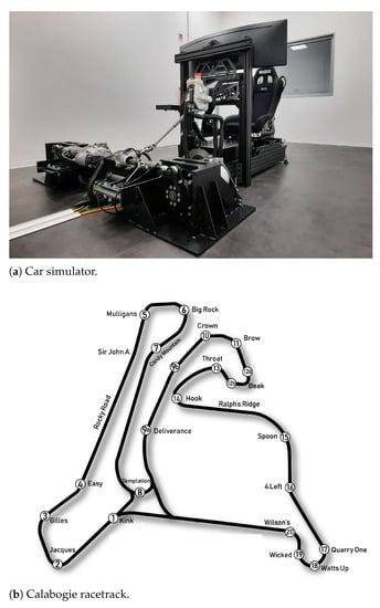
Figure 6.
Tests set-up.
The hardware characteristics and computational performance of the simulator are shown in Table 2 under the name Hardware 2.
In Table 2, it can be seen that the path planning computational time that resulted for both the hardware implementations is below the required specification of 0.1 s.
5.1. Comparison with Offline Motion Planning
These tests have involved the comparison of the architecture proposed with the max-performance event simulation of CRT suite. The max-performance simulation is used to define the dynamic speed limit profile on a given racetrack [26]. This offline simulation uses an iterative process where a specific static solver computes a velocity profile and then a dynamic solver verifies if the computed speed profile is feasible. Basically, the vehicle model used for static prediction has no suspensions and inherits all properties from the full CRT model. The effect of aero forces is considered and the effect of suspension jounce is taken into account by the presence of ride height maps, which link the dependency of ride heights to the vehicle velocity. The trajectory chosen to perform the max-performance event is that of minimum curvature of the Calabogie racetrack shown in Figure 6b. In the literature, this trajectory is often used as a reference, and it has been found that it is a trajectory that allows getting very close to the minimum lap time on a racetrack. For these tests, the simulation road is considered flat, neglecting the dynamics effects that the racetrack slopes and banks have on the performance.
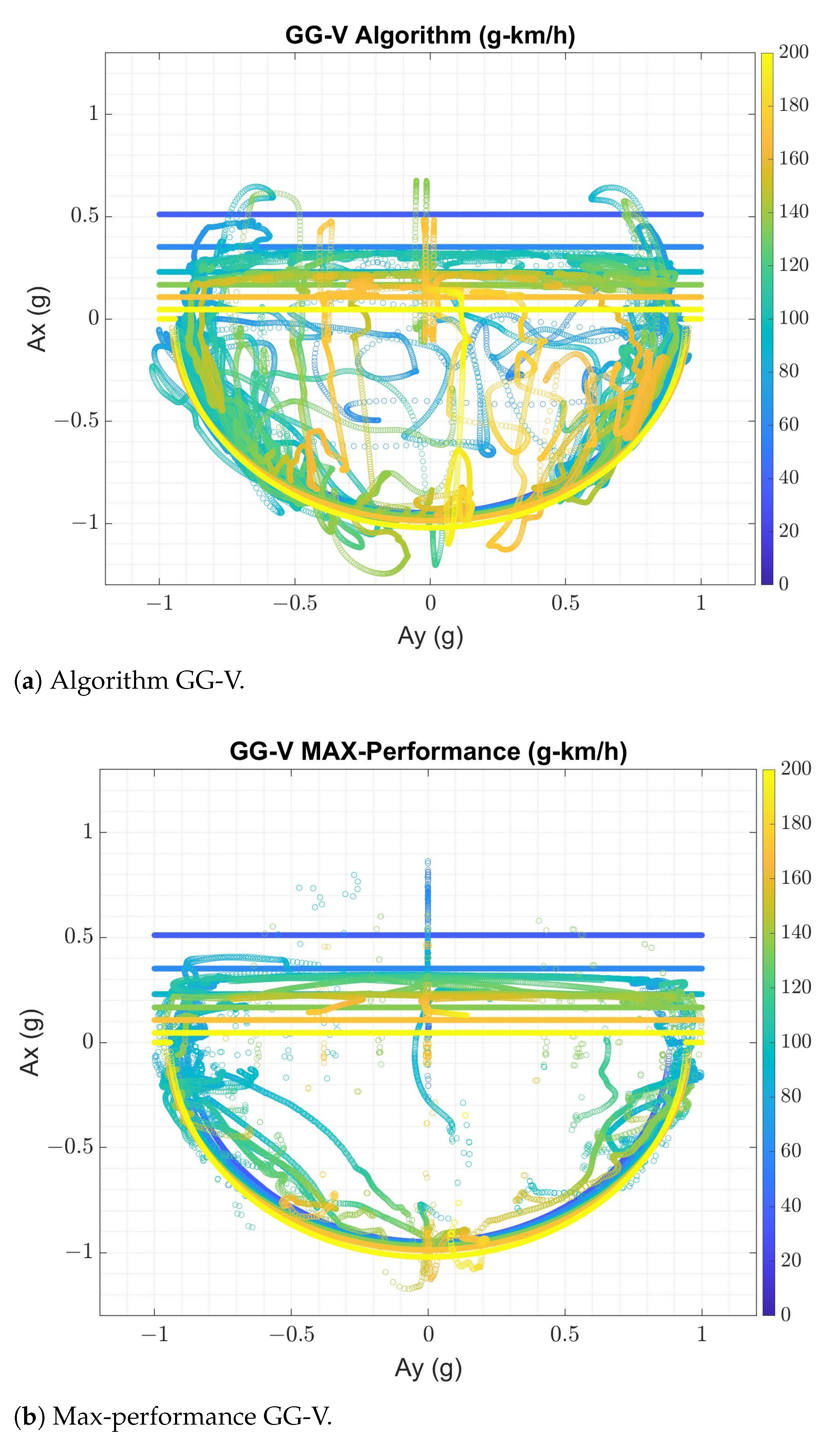
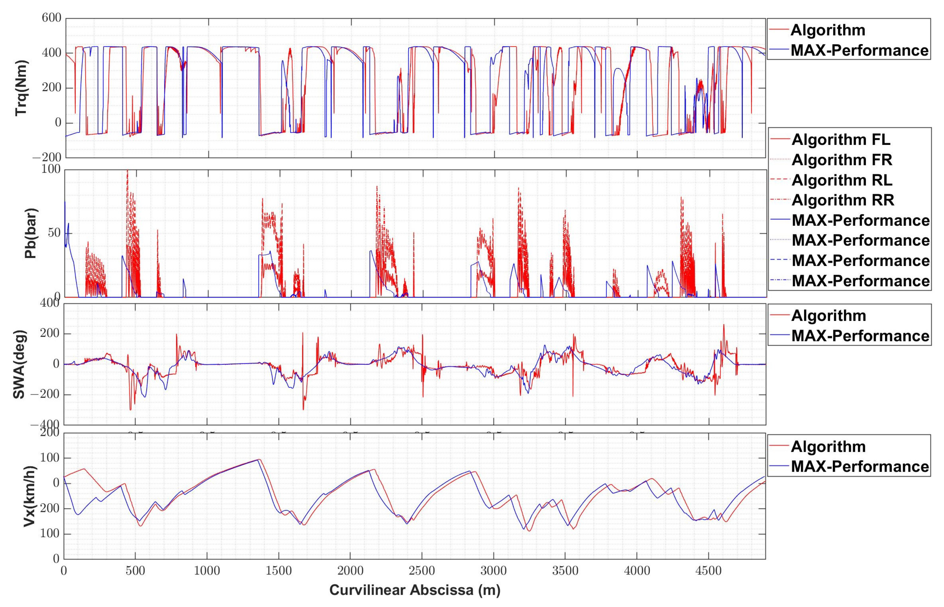
In Figure 7, the car’s longitudinal and lateral accelerations as a function of speed, GG-V, achieved by the car model controlled by the algorithm proposed and by the max-performance event are shown. In the same figures, the GG-V constraints implemented in the path planning are shown. By Figure 7b, it is possible to see that the constraints assumed in the trajectory tracking are representative of the car, and by Figure 7a, it is possible to see that the car controlled by the algorithm developed is able to keep the car inside the constraints imposed, even if with respect to the max-performance results, it goes through the transients more instead of staying within the limits of grip. This may be due to the inputs given to the vehicle being noisier than those of the offline control, as shown in Figure 8. Here, the engine torque, the chamber brake pressures and the steering wheel angle are almost similar in quantities with differences due to the different trajectory made, even if there is a visible difference in the amplitude and timing between the two configurations, i.e., the algorithm performed higher and delayed brake pressures with respect to the max-performance event. This is reflected in the speeds achieved by the car, which are almost similar, but the algorithm’s one brakes later, maintaining the high speed for more time than the max-performance speed, resulting in a reduction of lap time, as shown in Table 4.
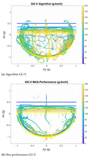
Figure 7.
Acceleration performance comparison.
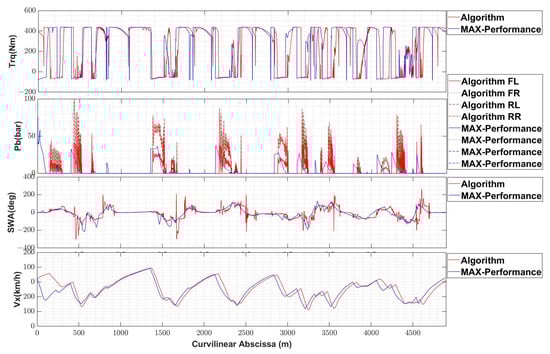
Figure 8.
Comparison of the input given to the vehicle and the output longitudinal speed between the algorithm proposed and the max-performance event.
Table 4.
Lap time performances.
5.2. Comparison with Driver
This second session of tests involved the comparison of the performance achieved by a professional driver and the trajectory tracking proposed. To perform these tests, the algorithm was compiled for use in the real-time simulator environment, and the road used is no longer flat but includes the actual lateral banks and longitudinal slopes of the road. For this reason, the longitudinal and lateral acceleration components due to the pitch and roll body movements and road inclination were added in the acceleration constraints of the path planning knowing the inclination of the road while the car is moving on the track and the pitch and roll of the car due to the brake, acceleration and steering states calculated as proportional to the difference between the front/right and rear/left normal wheel forces.
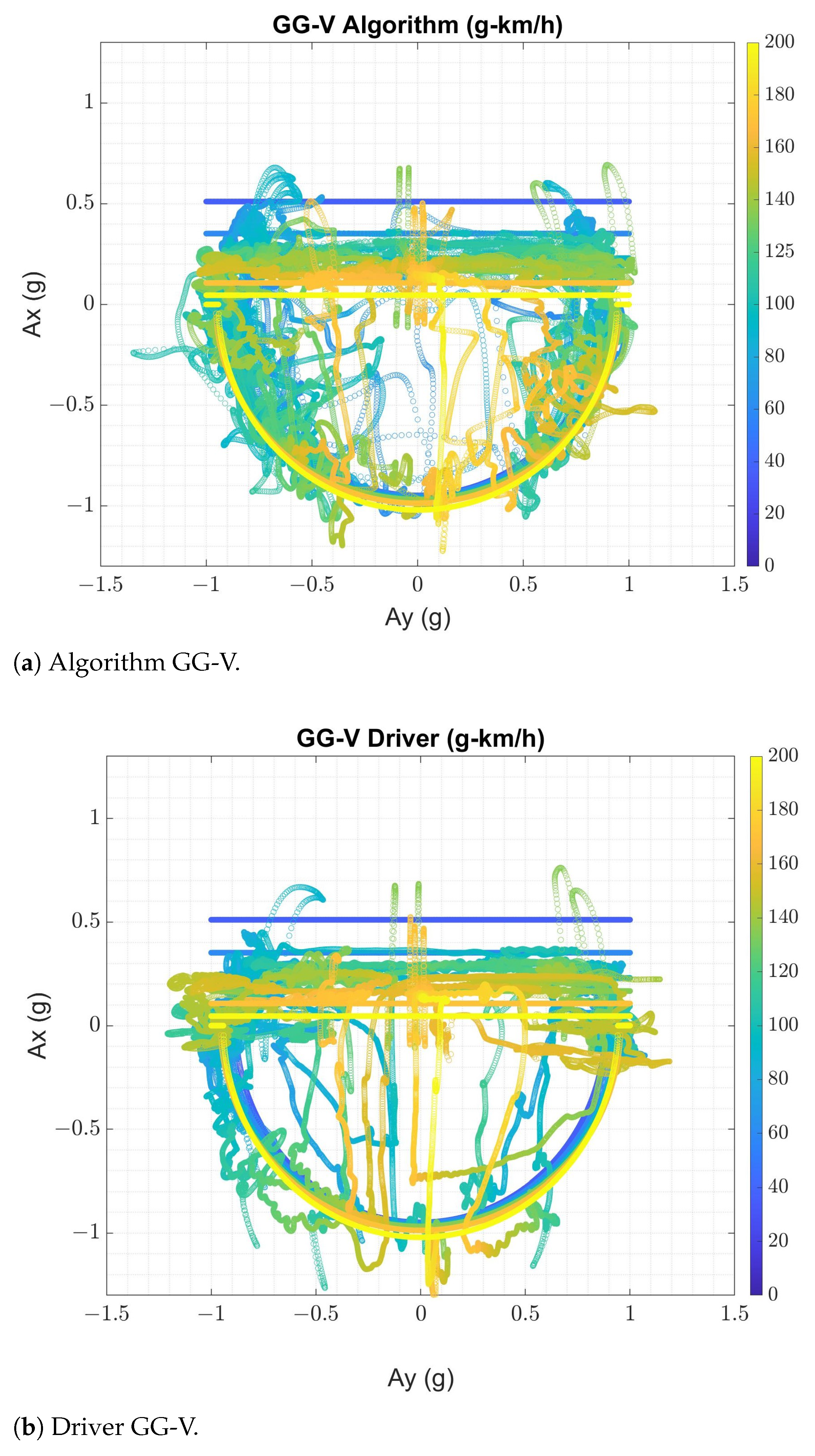
Looking at Figure 9, where the GGs obtained by the vehicle driven by the driver and by the algorithm are shown, it can be seen that the algorithm is able to respect the acceleration constraints imposed, by guaranteeing the limits of the engine and the tires and replicating the results obtained by the driver.
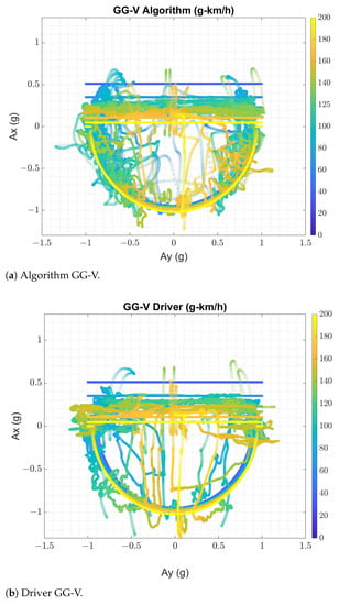
Figure 9.
Accelerations performance comparison.
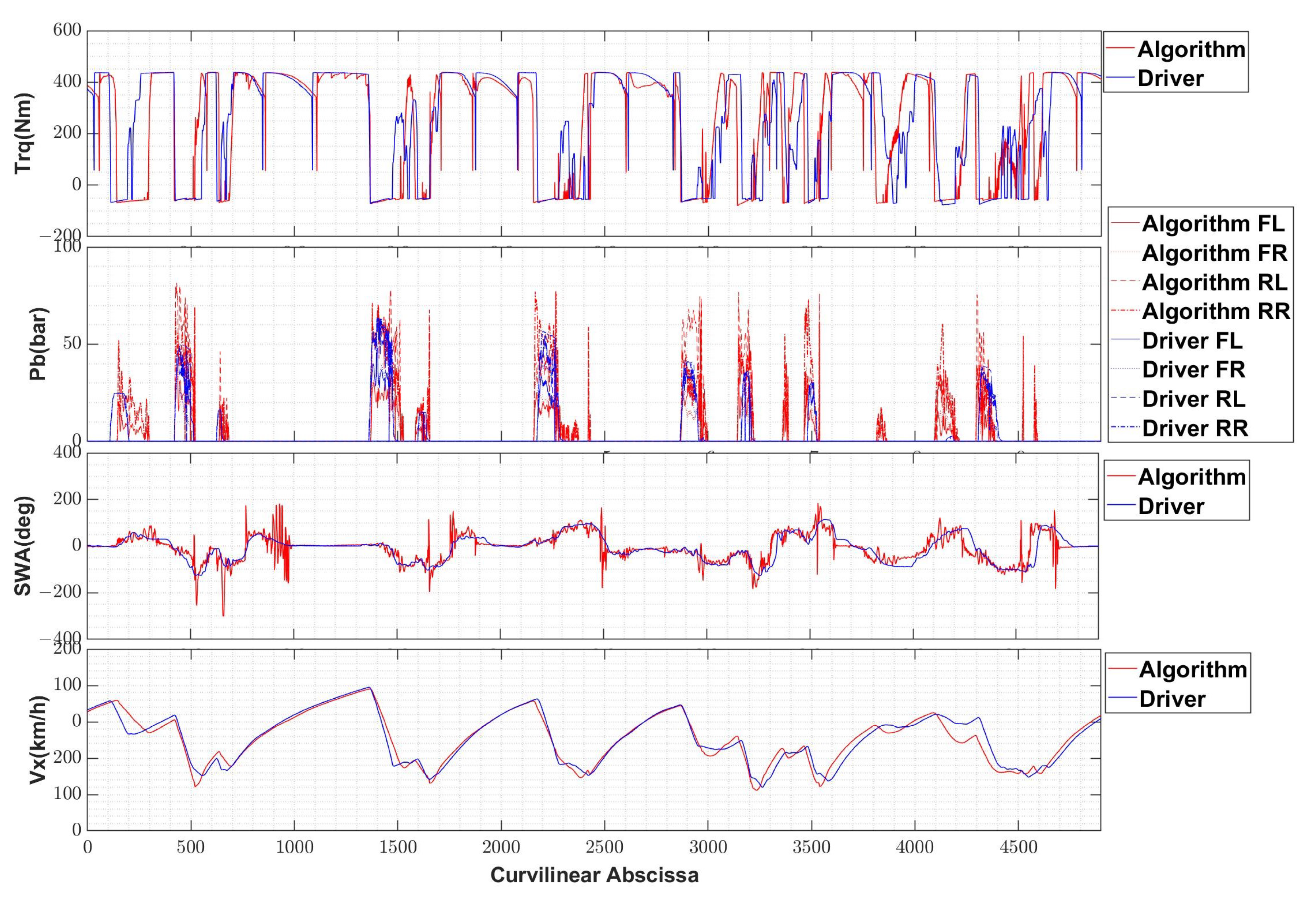
In terms of performance, the results show that the algorithm developed is able to match the ones of the professional driver, although simplifications have been made to the vehicle model to keep the computational cost down, in fact, speed and input curves have the same trend and peak values, as shown in Figure 10. The lap times shown in Table 4 confirm that the trajectory tracking developed is able to replace the results of a human driver, and that the system integration performs well.

Figure 10.
Comparison of the input given to the vehicle and the output longitudinal speed between the algorithm proposed and the driver.
5.3. Trajectory Comparison
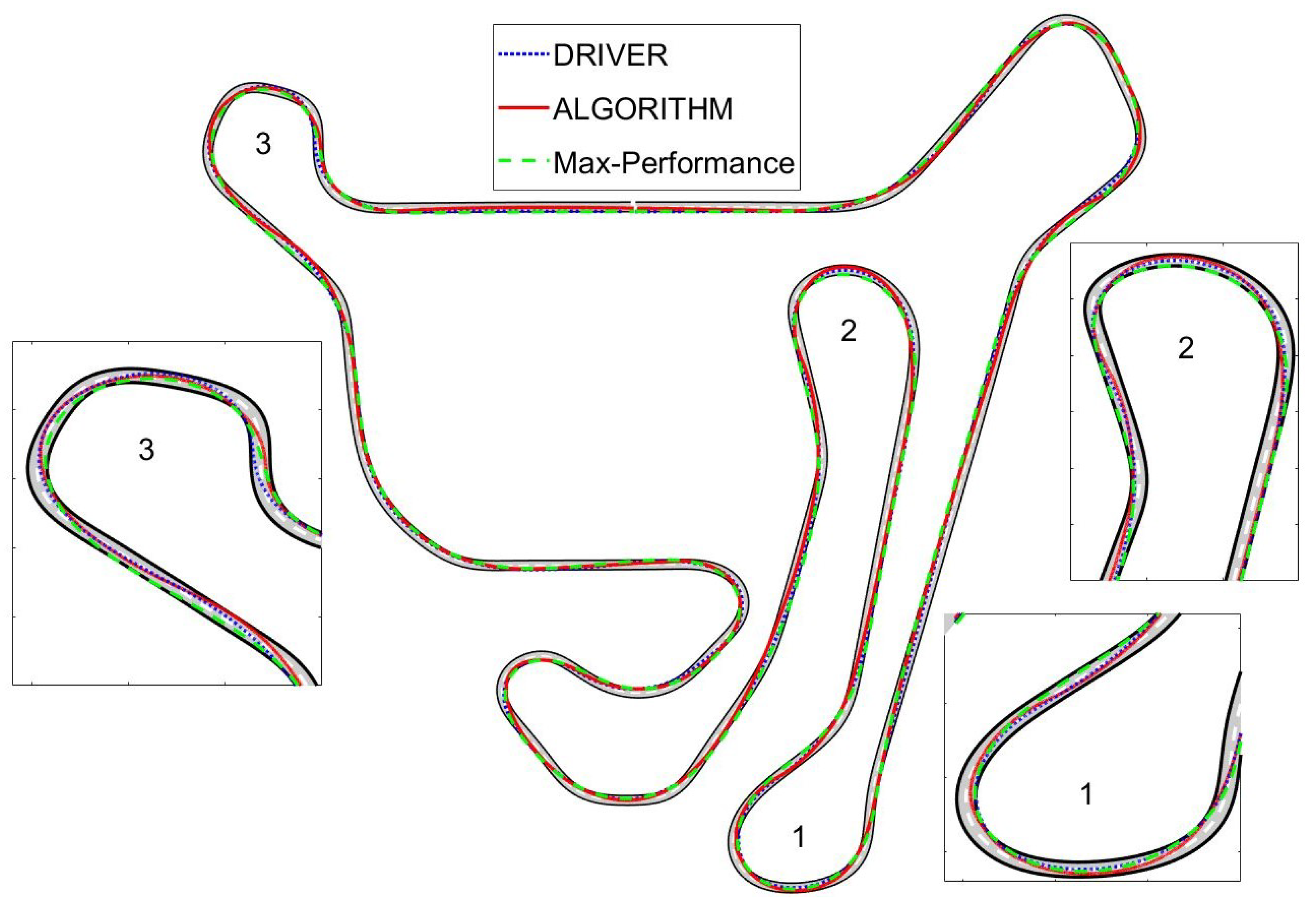
In Figure 11, the trajectories made by the algorithm developed, max-performance event and driver are compared, highlighting the curves where the different strategies are more visible and impact the performance. In zoom 1, it is possible to see that the trajectory of least curvature achieved by the offline optimization exits the curve keeping the car on the outer side of the track, whereas the proposed path planning drives the car to the inner side of the track to anticipate and prepare the car for the following curve, as the driver does, too. In this track section, the max normal distance between the trajectory made by the algorithm with respect to the one made by the max-performance event is 5.86 m; whereas, the one made by the driver can be considered equal to the algorithm one. In zoom 2, the different approaches are more visible and impact more on the performance: the trajectory of least curvature maintains the inner side, whereas the algorithm developed goes to the outer side, achieving a max normal distance of 8.00 m; this behavior was proved by driver tests, which improves the performance of the car and reduces the lap time, even if the driver made a trajectory 3.20 m closer than the algorithm. However, in zoom 3, if at the beginning of the curves, the max-performance optimization maintains the car on the outer side, and the driver and online algorithm choose the narrowest trajectory, achieving a max normal distance of 5.60 m, and at the end of the curves, the algorithm follows the max-performance, enlarging the trajectory later of almost 6.00 m with respect to the driver losing longitudinal speed.
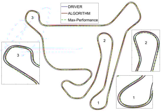
Figure 11.
Comparison of the trajectory made by the algorithm proposed and the driver.
6. Conclusions
In this paper, we developed an autonomous racing car trajectory tracker that was able to update the optimized trajectory online to reduce the time lap as well as control the car, and we validated this by comparing it with the performance of offline path planning and a human driver.
The intention of the paper was to ensure the online functionality of an autonomous controller to match the decisions of a human driver instead of optimizing the trajectory offline considering a possible development for an urban area.
This aim was achieved by dividing the path planning algorithm from the trajectory control one and building a hierarchical control architecture, where the vehicle model complexity increased and the sample time decreased, i.e., the path planning uses a point mass vehicle model with a sample time of 0.1 s, and the path tracking uses a single-track vehicle model with a sample time of 0.001 s. To ensure a correct communication between the two systems and the car, the computational time of the trajectory optimization was chosen to be below 0.1 s: the division between the path planning and path tracking and the implementation of LP instead of QP ensured the respect of these constraints, as shown in Table 2. Furthermore, to increase the path planning representation of the vehicle dynamic, the GG-V constraints were implemented as a quadratic ellipse, and the weights and the constraints of the optimization could be changed as a function of the track sections, adapting the car to the characteristics and conditions of the track. The comparisons made with a state-of-the-art offline path-planner validated the optimizer developed and the better performance achieved in terms of lap time, reducing it by almost a second.
The comparison made with a professional driver can prove that even if the autonomous architecture developed uses a simplified vehicle model to reduce the computational cost, the car is able to replicate its performance, matching the lap time.
In the future the Anti-Lock Brake System developed and published in [27] will be added to the control architecture to ensure an improvement in stability performance.
Author Contributions
Conceptualization and methodology, M.M. and L.R.; validation and data curation, M.M. and L.R.; writing—original draft preparation, M.M.; writing—review and editing, R.C. and C.A.; project administration, R.C. and C.A. All authors have read and agreed to the published version of the manuscript.
Funding
This research received no external funding.
Institutional Review Board Statement
Not applicable.
Informed Consent Statement
Not applicable.
Conflicts of Interest
The authors declare no conflict of interest.
Abbreviations
The following abbreviations are used in this manuscript:
| LP | Linear Programming |
| LQR | Linear Quadratic Regulator |
| QP | Quadratic Programming |
| MPC | Model Predictive Control |
| SCP | Sequential Convex Programming |
| DoF | Degrees of Freedom |
| PID | Proportional-Integral-Derivative |
| CRT | Car-Real-Time |
| UKF | Unscented Kalman Filter |
References
- Dal Bianco, N.; Bertolazzi, E.; Biral, F.; Massaro, M. Comparison of Direct and Indirect Methods for Minimum Lap Time Optimal Control Problems. Veh. Syst. Dyn. 2019, 57, 665–696. [Google Scholar] [CrossRef]
- Liniger, A. Path Planning and Control for Autonomous Racing. Ph.D. Thesis, ETH Zurich, Zurich, Switzerland, 2018. [Google Scholar]
- Liniger, A.; Domahidi, A.; Morari, M. Optimization-Based Autonomous Racing of 1:43 Scale RC Cars: OPTIMIZATION-BASED AUTONOMOUS RACING. Optim. Control Appl. Methods 2015, 36, 628–647. [Google Scholar] [CrossRef] [Green Version]
- Christ, F.; Wischnewski, A.; Heilmeier, A.; Lohmann, B. Time-Optimal Trajectory Planning for a Race Car Considering Variable Tyre-Road Friction Coefficients. Veh. Syst. Dyn. 2021, 59, 588–612. [Google Scholar] [CrossRef]
- Verschueren, R.; De Bruyne, S.; Zanon, M.; Frasch, J.V.; Diehl, M. Towards Time-Optimal Race Car Driving Using Nonlinear MPC in Real-Time. In Proceedings of the 53rd IEEE Conference on Decision and Control, Los Angeles, CA, USA, 15–17 December 2014; pp. 2505–2510. [Google Scholar]
- Verschueren, R.; Zanon, M.; Quirynen, R.; Diehl, M. Time-Optimal Race Car Driving Using an Online Exact Hessian Based Nonlinear MPC Algorithm. In Proceedings of the 2016 European Control Conference (ECC), Aalborg, Denmark, 29 June–1 July 2016; pp. 141–147. [Google Scholar]
- Alrifaee, B.; Maczijewski, J. Real-Time Trajectory Optimization for Autonomous Vehicle Racing Using Sequential Linearization. In Proceedings of the 2018 IEEE Intelligent Vehicles Symposium (IV), Changshu, China, 26–30 June 2018; pp. 476–483. [Google Scholar]
- Heilmeier, A.; Wischnewski, A.; Hermansdorfer, L.; Betz, J.; Lienkamp, M.; Lohmann, B. Minimum Curvature Trajectory Planning and Control for an Autonomous Race Car. Veh. Syst. Dyn. 2019, 2, 1497–1527. [Google Scholar] [CrossRef]
- Lot, R.; Dal Bianco, N. The significance of high-order dynamics in lap time simulations. In Proceedings of the 24th Symposium of the International Association for Vehicle System Dynamics (IAVSD 2015), Graz, Austria, 17–21 August 2015; Rosenberger, M., Plöchl, M., Six, K., Edelmann, J., Eds.; CRC Press: Boca Raton, FL, USA, 2016. [Google Scholar]
- Theodosis, P.A.; Gerdes, J.C. Generating a Racing Line for an Autonomous Racecar Using Professional Driving Techniques. In Proceedings of the ASME 2011 Dynamic Systems and Control Conference and Bath/ASME Symposium on Fluid Power and Motion Control, ASMEDC, Arlington, VA, USA, 31 October–2 November 2011; Volume 2, pp. 853–860. [Google Scholar]
- Perantoni, G.; Limebeer, D.J. Optimal Control for a Formula One Car with Variable Parameters. Veh. Syst. Dyn. 2014, 52, 653–678. [Google Scholar] [CrossRef] [Green Version]
- Gerdts, M. A Moving Horizon Technique for the Simulation of Automobile Test-Drives. ZAMM 2003, 83, 147–162. [Google Scholar] [CrossRef]
- Gerdts, M.; Karrenberg, S.; Müller-Beßler, B.; Stock, G. Generating Locally Optimal Trajectories for an Automatically Driven Car. Optim. Eng. 2009, 10, 439–463. [Google Scholar] [CrossRef]
- Timings, J.P.; Cole, D.J. Minimum Maneuver Time Calculation Using Convex Optimization. J. Dyn. Syst. Meas. Control 2013, 135, 031015. [Google Scholar] [CrossRef]
- Gurobi 8.1 Optimizer Reference Manual. 2018. Available online: https://www.gurobi.com/documentation/9.1/refman/index.html (accessed on 17 May 2020).
- Boyd, S.P.; Vandenberghe, L. Convex Optimization; Cambridge University Press: Cambridge, UK, 2004. [Google Scholar]
- Duchi, J. Sequential Convex Programming; Notes for EE364b; Stanford University: Stanford, CA, USA, 2018. [Google Scholar]
- Subosits, J.K.; Gerdes, J.C. From the Racetrack to the Road: Real-Time Trajectory Replanning for Autonomous Driving. IEEE Trans. Intell. Veh. 2019, 4, 309–320. [Google Scholar] [CrossRef]
- Guiggiani, M. The Science of Vehicle Dynamics: Handling, Braking, and Ride of Road and Race Cars, 2nd ed.; The Sciene of Vehicle Dynamics; Springer: Berlin/Heidelberg, Germany, 2018. [Google Scholar]
- Segers, J. Analysis Techniques for Racecar Data Acquisition, 2nd ed.; SAE International: Warrendale, PA, USA, 2014. [Google Scholar]
- Milliken, W.F.; Milliken, D.L. Race Car Vehicle Dynamics; SAE International: Warrendale, PA, USA, 1995. [Google Scholar]
- Pacejka, H.B.; Besselink, I. Tire and Vehicle Dynamics, 3rd ed.; Elsevier/Butterworth-Heinemann: Amsterdam, The Netherlands, 2012. [Google Scholar]
- Veneri, M.; Massaro, M. A Free-Trajectory Quasi-Steady-State Optimal-Control Method for Minimum Lap-Time of Race Vehicles. Veh. Syst. Dyn. 2019, 58, 1–22. [Google Scholar] [CrossRef]
- Altche, F.; Polack, P.; de La Fortelle, A. A Simple Dynamic Model for Aggressive, near-Limits Trajectory Planning. IEEE Intell. Veh. Symp. 2017, IV, 141–147. [Google Scholar]
- Rajamani, R. Vehicle Dynamics and Control; Springer Science: Berlin/Heidelberg, Germany, 2006. [Google Scholar]
- VI-CarRealTime 18.2 Web Help Documentation; VI-Grade GmbH: Darmstadt, Germany, 2018.
- Montani, M.; Vitaliti, D.; Capitani, R.; Annicchiarico, C. Performance Review of Three Car Integrated ABS Types: Development of a Tire Independent Wheel Speed Control. Energies 2020, 13, 6183. [Google Scholar] [CrossRef]


Publisher’s Note: MDPI stays neutral with regard to jurisdictional claims in published maps and institutional affiliations. |
© 2021 by the authors. Licensee MDPI, Basel, Switzerland. This article is an open access article distributed under the terms and conditions of the Creative Commons Attribution (CC BY) license (https://creativecommons.org/licenses/by/4.0/).