Abstract
Reducing the energy consumption of the heating, ventilation, and air conditioning (HVAC) systems while ensuring users’ comfort is of both academic and practical significance. However, the-state-of-the-art of the optimization model of the HVAC system is that either the thermal dynamic model is simplified as a linear model, or the optimization model of the HVAC system is single-timescale, which leads to heavy computation burden. To balance the practicality and the overhead of computation, in this paper, a multi-timescale bilinear model of HVAC systems is proposed. To guarantee the consistency of models in different timescales, the fast timescale model is built first with a bilinear form, and then the slow timescale model is induced from the fast one, specifically, with a bilinear-like form. After a simplified replacement made for the bilinear-like part, this problem can be solved by a convexification method. Extensive numerical experiments have been conducted to validate the effectiveness of this model.
1. Introduction
It has been well known that heating, ventilation, and air conditioning (HVAC) systems, which are widely applied to various buildings, directly affect the user’s comfort and are responsible for a large proportion of the building’s energy consumption. Over the last several years, the problem of optimizing the energy consumption of HVAC systems while ensuring user’s comfort has been extensively investigated [1,2,3,4].
In an HVAC system, the thermal dynamics of a residential house may be modeled at a minute level, while the load profile for the maximum power consumption is usually specified at an hourly level. If the optimization problem of the HVAC system is modeled in single-timescale, the time should be slotted with the length of the smallest timescale (e.g., minute). Clearly, in this case, the number of decision variables increases dramatically, which leads to the curse of dimensionality [5,6,7]. In addition, the thermal dynamic model of the HVAC systems in a building is complex, which may further increase the dimension of optimization problem and the computational complexity [8,9,10,11,12]. References [13,14] proposed a two-timescale stochastic optimization model for control and scheduling the appliances to satisfy user’s thermal comfort requirement under the peak power and cost constraints. The two-timescale model could efficiently reduce both the dimension of the problem and its computational complexity. Despite the two-timescale models in [13,14] can appropriately characterize the optimization problem of HVAC systems, the consistency of the models in two timescales was not guaranteed. To solve this problem, article [15] improved these two-timescale models and developed a two-timescale induced model to ensure the consistency. The consistency mentioned above refers to the consistent models established no matter it is the fast timescale model obtained by decomposing the slow timescale model or the slow timescale model induced reversely from the fast timescale model.
In the above-mentioned research, the thermal dynamic model is simplified as a linear model. Although the linear models are easy to solve, the bilinear models are more practical to describe the thermal dynamics of buildings [16,17,18,19,20]. In [16], a Swiss office building was formulated as a bilinear model to analyze its implementation, results, and cost–benefit under model predictive climate control. In [17], a problem of HVAC control in a typical commercial building was studied, which was formulated as a bilinear model. At present, there already exist some mature algorithms for bilinear system optimization, e.g., dynamic planning and maximum principle. In [18], a sequential quadratic programming method was proposed to solve bilinear HVAC control problems, which is computationally expensive for nonconvex problems and needs a good initialization to achieve local convergence. In [19,20], a convex relaxation method is developed to reduce the computation burden efficiently. The bilinear models in the above articles are modeled in single-timescale.
To make a trade-off between the practicality and the overhead of computation, this paper formulates the optimization problem of HVAC system as a multi-timescale bilinear model. In [15], a multi-timescale linear model is built. The current paper extends the results in [15] to a multi-timescale bilinear model, which is more practical to describe the thermal dynamics of HVAC systems. However, the coupling of multi-timescale and bilinearity makes the induced slow timescale model not be the standard bilinear form. The relationship between the slow timescale model and fast timescale model is clarified, and then the multi-timescale bilinear model can be solved by the convexification method after simplified replacement. In addition, a multi-timescale deterministic model is adopted in this paper against the mixture of the inconsistency deviation and the random error.
The contribution of this paper is formulating the multi-timescale bilinear optimization model of HVAC systems to balance the practicality and the overhead of computation. Based on the induction method for multi-timescale model in [15], the fast timescale bilinear model is built first, and then the slow timescale model is induced from the fast one, in which the consistency of models in different timescales is guaranteed. Compared with single-timescale bilinear models, the proposed model can decrease the computational complexity; while compared with multi-timescale linear models (e.g., [15]), the proposed model can describe the thermal dynamic of HVAC systems more practically and get better optimization results in some cases, and the accuracy and the computational cost are acceptable.
The remainder of this paper is outlined as follows. In Section 2, the multi-timescale HVAC bilinear induced model is formulated. In Section 3, the solution algorithm is introduced. In Section 4, the performance of the proposed strategy is illustrated through case studies. In Section 5, we conclude this paper. Due to space limitation, proofs of theorems are omitted and can be found in [21].
2. Problem Formulation
2.1. Single-Timescale Bilinear Optimization Model
An HVAC system draws power and drives the indoor temperature by following a thermal dynamic model, and the HVAC control directly affects the user’s comfort. The user’s comfort in this paper reflects that the deviation from the indoor temperature and the desired temperature of the user is minimized. This paper regulates the indoor temperature by control and decision for HVAC.
Based on a practical building, the HVAC optimization model is built as follows, in which the objective is to improve user’s comfort with limited energy. The details can be seen in our previous work [15] and are not repeated here. For simplicity, some random factors are not considered in this paper.
where xk is the indoor temperature at time k. dk is the user’s desired temperature at time k. uk is the control variable of HVAC at time k. umax denotes the maximum limit of control variable of HVAC. Umax denotes the maximum total limit of control variable of HVAC. a, b, c are coefficients.
(P1) min ∑|xk − dk|
s.t.xk+1 = axk + buk + cxkuk
0 ≤ uk ≤ umax
∑uk ≤ Umax
Constraint (2) is a bilinear state transfer equation. Bilinear system is a kind of system derived by introducing the product term of state variable and control variable in linear state equation. It is relatively linear to state variable and control variable, respectively, but not linear to state variable and control variable simultaneously. In fact, bilinear system is a special nonlinear system with simple form. Bilinear system model is a promotion from linear system model, which can more practically describe the indoor temperature state transfer process.
In the system, the time domain is divided into two timescales, as shown in Figure 1, where K is the number of time slot in slow timescale, and n is the number of time slot in fast timescale of slow timescale. According to [15], states transfer in fast timescale, that is, the model in (P1) is the fast timescale model, and the slow timescale model should be induced by it.
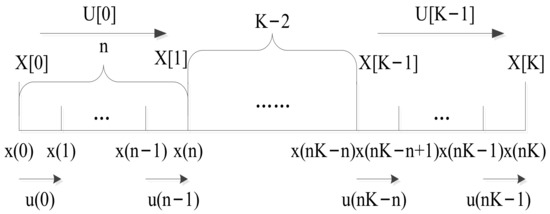
Figure 1.
Slow timescale and fast timescale diagram.
2.2. Two-Timescale Bilinear induced Model
For simplicity, we select one interval of slow timescale, including four slots of fast timescale, as shown in Figure 2.

Figure 2.
One interval of slow timescale.
The standard bilinear state transfer equation of fast timescale is known as (2).
The relationship between state variables of slow timescale and fast timescale is assumed as follows.
X[0] = x0, X[1] = x4
When the slow timescale state transfers from X[0] to X[1], the fast timescale state transfers from x0 to x4, both of them transfer n times fast timescales.
According to the fast timescale state transfer equations, this transfer process can be described as
Combine (5) with (6) we can obtain the slow timescale state transfers from X[0] to X[1] as follows.
The slow timescale bilinear state transfer equation should have been the same form as fast timescale, however, unless in the particular condition that a = 1, there does not exist a uniform control variable U[k] in (7). In other words, the control variables in control term and bilinear term are different, so we describe the two as UB[k] and UC[k], respectively. UB[k] is the second term at the right-hand side of (7), and x0UC[k] is the third term. Comparing UB[k] with UC[k], we find that the former still carries the quality of weighted sum with coefficient a, while the latter reflects such quality similar to simple sum 15.
Therefore, unlike the linear system in our previous work, the slow timescale state transfer equation of bilinear system cannot be described as the standard bilinear state transfer equation, but a bilinear-like form as follows.
where X[k] is the indoor temperature at kth slow timescale. A, B, C are coefficients in slow timescale.
X[k + 1] = AX[k] + BUB[k] + CX[k]UC[k]
To extend n = 4 to general cases, we formulate the following theorems.
Theorem 1.
The fast timescale system state equation is (2). The relationship between state variables of slow timescale and fast timescale is X[k] = xnk. Thus, the slow timescale system state equation can be induced as (8), where the coefficients are
A = an, B = b, C = c
The slow timescale control variable is
Proof of Theorem 1.
See [21]. □
In this mode, UB[k] and UC[k] indicate two different kinds of control effect.
Corollary 1.
By solving the slow timescale model, the control variable is obtained with a set of unk decomposition, i.e., (10). Thus, the decision is realizable in the fast timescale, in other words, there is a set of fast timescale state transfer as X[k] = xnk.
Theorem 2.
The fast timescale system state equation can be described as the standard bilinear system state Equation (2), and the relationship between the state variables of slow timescale and fast timescale is X[k] = xnk. When a ≠ 1, there does not exist two same U[k], making the slow timescale system state equation have the standard bilinear form like (2).
Proof of Theorem 2.
See [21]. □
2.3. Two-Timescale Bilinear Optimization Model
Based on the proposed theorems in last section, the two-timescale bilinear optimization model is built as follows.
Slow timescale:
where D[k] is the desired temperature at kth slow timescale. Uc[k] denotes the total of fast timescale control variables of HVAC at kth slow timescale, which is an actual physical quantity.
(P2) min ∑|X[k] − D [k]|
s.t. (8), (10)
0 ≤ Uc[k] ≤ Umax
Constraint (12) expresses the energy conversation law. Constraint (13) restricts the maximum limit of the actual consumption of HVAC in the slow timescale.
Fast timescale:
s.t.xnk+1 = axnk + bunk + cxnkunk
0 ≤ uk ≤ umax
Constraint (15) ensures that fast timescale state/control variables satisfy the bilinear state transfer equations. Constraint (10) ensures the consistency of decomposition from the slow timescale to the fast timescale. Constraint (17) ensures that the total consumption of control variables in this period shall not exceed that in the scheduling plan of slow timescale.
3. Convexification Solution Method
The aforementioned optimization problem is nonconvex due to the bilinear term. To solve this issue, a convex relaxation method is used in this section.
3.1. Simplified Constraint
Before convexification, constraint (10) is so complicated that should be simplified to solve. We find that both UB[k] and UC[k] consist of first-order term to n-order term of u. The terms are divided into n = 6 parts in Table 1.

Table 1.
Terms in U[k].
According to the physical meaning of the system, the state variable denotes indoor temperature, the control variable u is related to air flow rate of HVAC, a is a self-loss coefficient, b denotes air temperature from HVAC, K is the number of time slot in slow timescale, so values of u of HVAC are always small rated with other variables. The value of the fourth-order term tends to 0, so the fifth-order to nth-order terms can be ignored. Although the values of second-order term to fourth-order term are small, with numbers of these terms not small, they cannot be ignored simply. For example, the number of u’s second-order terms is , the number of u’s third-order terms is , etc. However, also because these terms have little influence on the whole formula, they can be replaced by two constant terms, CB[k] and CC[k], for UB[k] and UC[k], respectively. In other words, S1 remains and S2–S4 is replaced by CB[k] and CC[k]. Constraint (10) is changed as follows.
UB[k] ≈ an−1u0 + an−2u1 + … + un−1 + CB[k]
UC[k] ≈ an−1(u0 + u1 + … + un−1) + CC[k]
UC[k] ≈ an−1(u0 + u1 + … + un−1) + CC[k]
In this mode, UB[k] is not the simple sum of u, but the weighted sum with coefficient a. UC[k] has a linear relationship with the simple sum of u, i.e., the actual energy consumption, a physical quantity.
Let all u of S2–S4 equal ue[k], the values of S2–S4 in UB[k] and UC[k] equal CB[k] and CC[k], respectively. ue[k] means the control variable that is needed over one slot in fast timescale to keep the desired temperature at kth slow timescale. Namely, the state variable in (15) is replaced with the desired temperature D[k], as follows.
D[k] = aD[k] + bue[k] + cD[k]ue[k]
We will make a preliminary estimate roughly whether user can accept the error from the above replacement. Firstly, S2/S1 ≈ u2/nu = (n − 1)u/2. For example, u ranges [0.05, 0.15], n = 6, S2/S1 ≈ 0.125~0.375. With the value of u small, S2/S1 is small, i.e., the changes of S2 have little influence on S1 + S2. The absolute value of relative error of S2 changed before and after is estimated as follows.
where δ denotes the deviation between ue and u, and is generally an order magnitude smaller than u. |δ| is from 0 to [0.005, 0.015], so δ2 can be ignored. Equation (21) is transformed as follows.
|εS2| = |2 C2nuδ + C2nδ2|/(nu + C2nu2) = |δ|/(1/n − 1 + u/2)
Considering the ranges of u and δ, |εS2| is estimated as 0~[0.02, 0.05]. Thus, the influence of S2 replaced before and after is little for the formula. For the same reason, the influences of S3 and S4 decrease progressively. It will be further illustrated through numerical examples in Chapter IV.
Then, in order to further simplify Equation (10), let ζB[k] = (an−1 + … + 1)ue[k], ζC[k] = nan−1ue[k], we can obtain
CB[k] = c[dζB[k]/da]ue[k] + … + (ci/i)[diζB[k]/dai]uei[k] + … + (cn−1/n − 1) [dn−1ζB[k]/dan−1]uen−1[k]
CC[k] = c[dζC[k]/da]ue[k] + … + (ci/i)[diζC[k]/dai]uei[k] + … + (cn−1/n − 1) [dn−1ζC[k]/dan−1]uen−1[k]
3.2. Convex Relaxation Method
Another computational issue is the bilinear model always results in nonconvex optimization problem. To solve this issue, some convex relaxation method will be developed.
McCormick Envelopes is a common method of convex relaxation used in bilinear nonlinear programming problem [19,20,22,23,24,25]. According to the method, the bilinear term can be bounded by its convex and concave envelopes. We need to confirm the upper and lower bound of the bilinear term first.
The optimization objective is to minimize the deviation from indoor temperature and the user’s desired temperature, so state variable is constrained within the scope above and below near the user’s desired temperature.
dk − Δ ≤ xk ≤ dk + Δ
The upper and lower bound of control variable is (16).
Therefore, the bilinear term xkuk is bounded by
xkuk ≥ max{(dk − Δ)uk, (dk + Δ)uk + umaxxk − umax(dk + Δ)}
xkuk ≤ min{umaxxk + (dk − Δ)uk − umax(dk − Δ), (dk + Δ)uk}
The nonconvex problem can be relaxed by replacing the bilinear term xkuk with an additional variable yk. The relaxed state transfer equation is
xk+1 = axk + buk + cyk
Additional constraints are needed as follows.
0 ≤ (buk + cyk)/(b + cxk) ≤ umax
It is worth noting that the above convex relaxation method is applied to fast timescale under the default condition, yk = xkuk. However, for slow timescale, there is not Y[k] = X[k]U[k].
The bilinear term in slow timescale is X[k]UC[k], which can also be bounded by its convex and concave envelopes. We confirm its upper and lower bound first.
Similarly, state variable of slow timescale is constrained within the scope above and below near the user’s desired temperature.
D[k] − Δ ≤ X[k] ≤ D[k] + Δ
According to (12), (13) and (18), we can obtain the upper and lower bound of UC[k] as follows.
CC[k] − Δ ≤ UC[k] ≤ an−1Umax + CC[k]
Therefore, the bilinear term X[k]UC[k] is bounded by
Let Y[k] = X[k]UC[k], the relaxed slow timescale state transfer equation is
X[k + 1] = AX[k] + BUB[k] + CY[k]
Additional constraint is needed as follows.
CC[k] ≤ (BUC[k] + CY[k])/(B + CX[k]) ≤ an−1Umax + CC[k]
Moreover, according to Theorem 1 in 15, there are U*[k] and Y*[k] satisfying
U*[k] = UB[k] − CB[k] = an−1unk + an−2unk+1 + … + unk+n−1
Y*[k] = Y[k] + (B/C)CB[k] = an−1uynk + an−2ynk+1 + … + ynk+n−1
To guarantee the consistency of the two-timescale model, additional constraint is needed as follows.
3.3. Relaxed Two-Timescale Bilinear Optimization Model
With the aforementioned additional constraints, a modification of (P2)(P3) is proposed below.
Slow timescale:
(P4) min ∑|X[k] − D [k]|
s.t. (12), (13), (18), (35), (36)
Y[k] ≥ CC[k]X[k] + (D[k] − Δ)UC[k] − CC[k](D[k] − Δ)
Y[k] ≥ (D[k] + Δ)UC[k] + (an−1Umax + CC[k])X[k] − (an−1Umax + CC[k])(D[k] + Δ)}
Y[k] ≤ (an−1Umax + CC[k])X[k] + (D[k] − Δ)UC[k] − (an−1Umax + CC[k])(D[k] − Δ)
Y[k] ≤ (D[k] + Δ)UC[k] + CC[k]X[k − CC[k](D[k] + Δ)}
Fast timescale:
s.t. (16), (17), (28)–(30), (37)–(39)
yk ≥ (dk − Δ)uk
yk ≥ (dk + Δ)uk + umaxxk − umax(dk + Δ)
yk ≤ umaxxk + (dk − Δ)uk − umax(dk − Δ)
yk ≤ (dk + Δ)uk
The solution methodology for the two-timescale optimization problem has been described in our work [15] in details. In brief, after removing the absolute value sign of the objective functions, the slow timescale optimization problem is solved first, and then the fast timescale optimization problem is solved with the results of slow timescale. Based on the linear constraints, we formulate the relaxed model as a linear programming (LP) problem, which can be efficiently solved using Cplex.
4. Numeric Results
In this chapter, we demonstrate the performance of the two-timescale bilinear optimization model on an HVAC system. For simplicity, we choose one of rooms to illustrate, where a = 0.95, b = 38, c = −1, n = 6, K = 16.
4.1. Error Analysis
The error analysis in this section is aimed at the simplified replacement mentioned in III-A. To highlight the problem, we select the kth slow timescale, where X[k] = xnk = 24, D[k + 1] = 25, Δ = 0. According to (10),
UB[k] = (a5u0 + a4u1 + … + u5) + (a4cu0(u1 + … + u5) + a3cu1(u2 + … + u5) + cu4u5) + … + c5u0u1u2u3u4u5
UB[k] = a5(u0 + … + u5)+ a4c(u0(u1 + … + u5)+ u1(u2 + … + u5) + u4u5) + … + c5u0u1u2u3u4u5
Solving the kth slow timescale optimization, we can obtain a set of u = [u0, …, u5], and then the numerical values of S1–S6 are shown in Table 2.

Table 2.
The Contrast of Replacement Before and After.
Let U^[k] = BUB[k]CX[k]UC[k], and X[k + 1] = AX[k] + U^[k]. The absolute values of relative error for U^[k] and X[k + 1] is calculated as follows, respectively.
|εU^[k]| = |U^[k] − U^’[k]|/U^[k]
The numerical results are shown in Table 3.

Table 3.
Absolute Value of Relative Errors.
Although |εU^[k]| = 4.39%, |εX[k+1]| = 1.29% merely, indicating that final output of state is weakly affected. In terms of indoor temperature, 1.29% error is almost imperceptible for user body.
Moreover, we compare the situation1 that simply deletes S2–S6 with the aforementioned situation 2 during the whole optimization process. The indoor temperature of the original formula is regarded as the standard compared with those in the two situations, and the mean absolute percentage error (MAPE) is calculated as follows [26].
The MAPE of state variable are contrasted in Table 4.

Table 4.
MAPE1.
In summary, the error from the way we make the simplification is acceptable.
4.2. Accuracy
The accuracy of the proposed optimization solution will be discussed in this section.
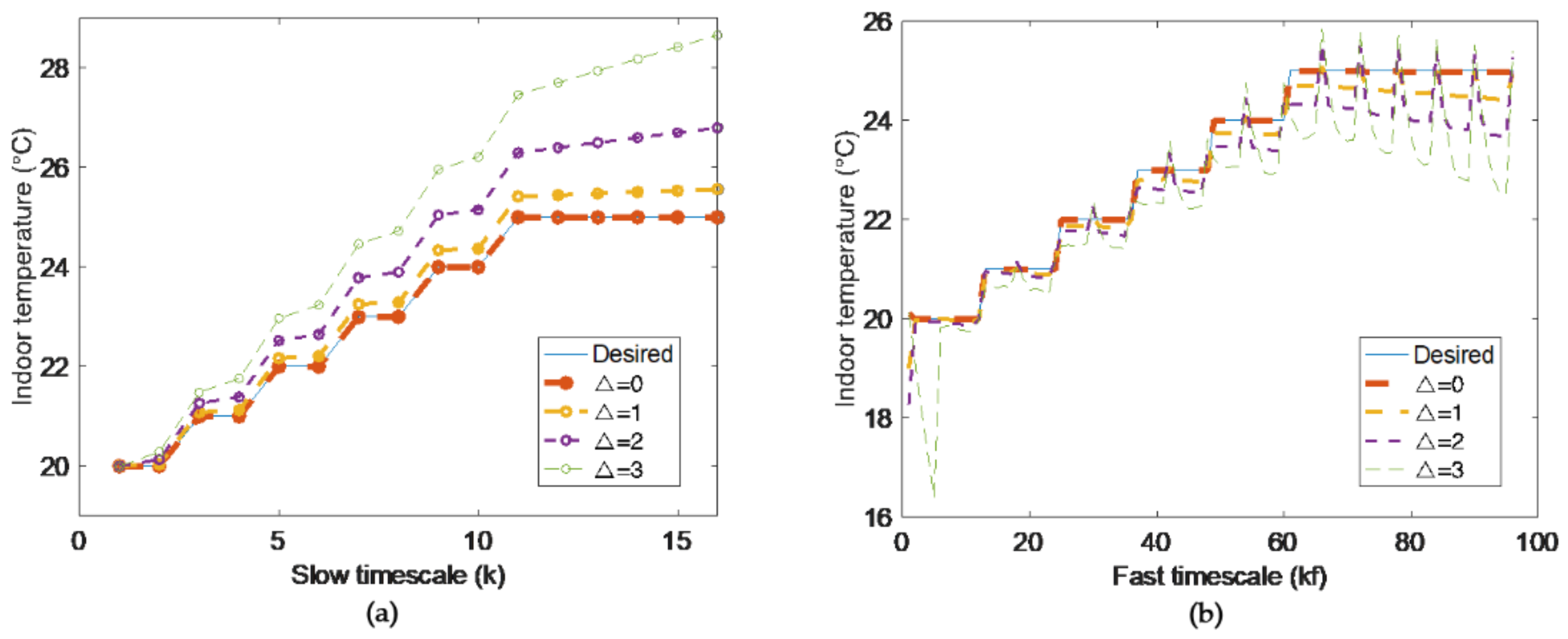
Through simulation, it is found that the value of Δ can directly affect the accuracy of optimization result from the proposed model. The less Δ values, the more accuracy will be. With the decrease of Δ, the range of state variable becomes less, and the bound by convex and concave envelopes is more practical.
The actual indoor temperature from simulation is compared with user’s desired temperature and MAPE is calculated for each Δ. The MAPE formula is shown as follows, which sums up all the absolute percentage error for one value and then finds the average.
When Δ = 0, 1, 2, 3, respectively, the MAPEs are shown in Table 5, where Δ = 0 for reference only.

Table 5.
MAPE2.
Under different values of Δ, the accuracy of the proposed model are contrasted in Figure 3.
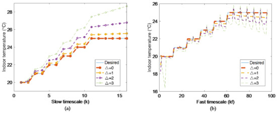
Figure 3.
Model in slow timescale (a) and fast timescale (b).
Figure 3 shows the states and the desired temperature under different values in the slow timescale and fast timescale. We see that the deviation from desired temperature become more with the increase of Δ. When Δ < 3, deviations are acceptable.
4.3. Comparison with The Linear Model
The results obtained from the proposed bilinear model are compared with those obtained from the linear model in [15]. It should be pointed out that the linear model in [15] is a Jacobian linearization [27] of the bilinear model in the current paper, i.e., the dynamics at every time step are linearized around the equilibrium points of the system. Next, the performances of linear model and bilinear model are compared through numerical results.
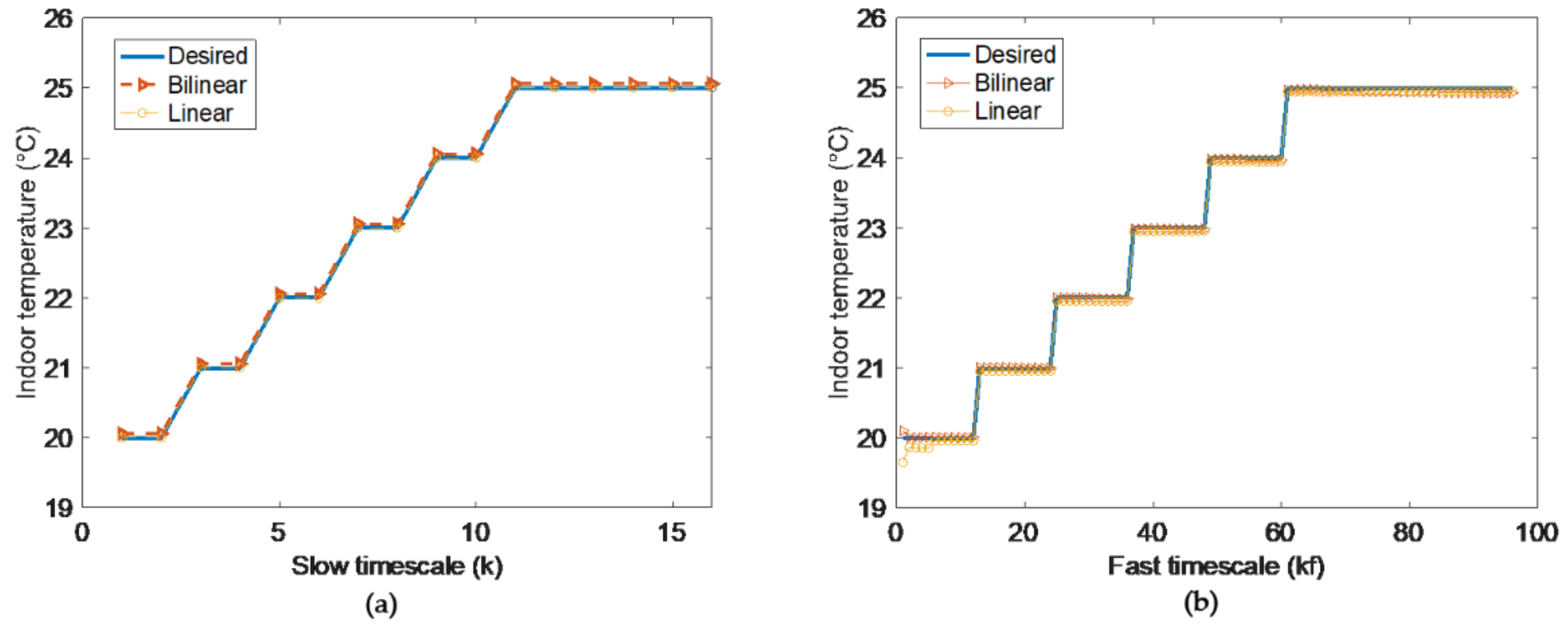
If the indoor temperatures at all time could satisfy the desired temperatures, as shown in Figure 4, there does not exist linearization error in the linear model, so whose performance is good in our previous work. Generally speaking, the indoor temperature in slow timescale can meet the desired temperature with sufficient energy budget. However, when the decision result of slow timescale is decomposed in fast timescale, only the states of endpoint in fast timescale can be guaranteed, and the other states would transfer to the endpoint through arbitrary paths, i.e., except the states of endpoint, not all of the other states can meet the desired temperature [15]. At this time, deviation occurs in fast timescale linear model.
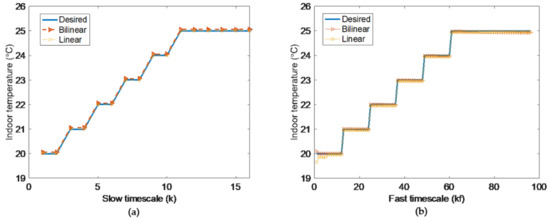
Figure 4.
Two-timescale indoor temperatures in bilinear model (a) and linear model (b).
In the cases mentioned above, the optimization results of the bilinear model and linear model are shown in Figure 5. In slow timescale, we see that all states of linear model satisfy the desired temperatures, and the states of bilinear model also behave well with just acceptable little error. However, in fast timescale, if user set the desired temperatures with fluctuation at the first two periods (k = 1–2) of slow timescale (i.e., kf = 1–12 of fast timescale), and the desired temperatures at the endpoints (kf = 6, 12) coincide with that in slow timescale (k = 1, 2), there will be great deviation in linear model. Once state cannot meet the desired temperature, linear model will make the following optimization process based on a biased model after that. Since bilinear model is built in practice, following the practical situation well, it can satisfy the desired temperatures within acceptable scope.
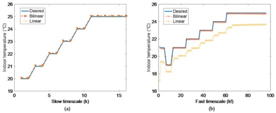
Figure 5.
Two-timescale indoor temperatures in bilinear model (a) and linear model (b) with fluctuant desired temperatures.
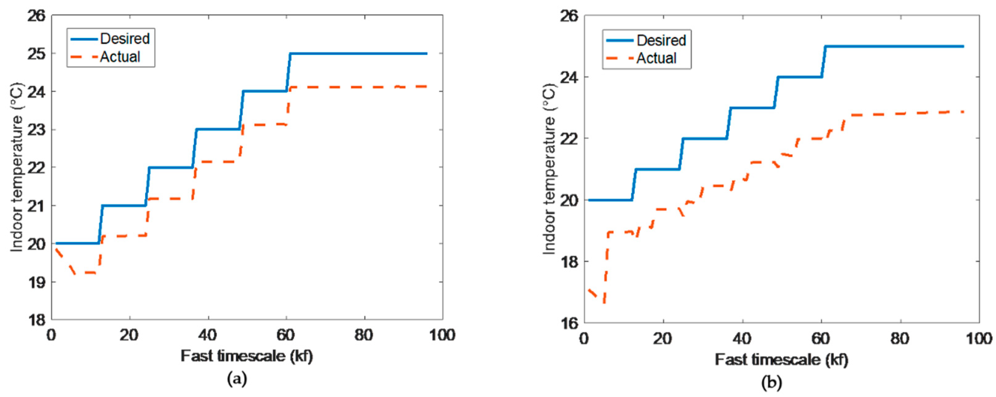
Under some special circumstances with not sufficient energy budget, where the main aim is not for user comfort, the optimization results are shown in Figure 6.
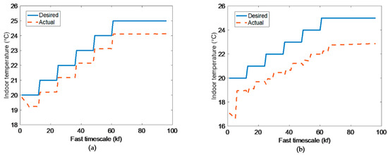
Figure 6.
Fast timescale indoor temperatures in bilinear model (a) and linear model (b).
Because of insufficient energy, states cannot satisfy the desired temperatures both in bilinear model and linear model. As shown in Figure 6, it is obvious that the optimization result of bilinear model is better than linear model.
Extensive simulation experiments have been carried out. The results show that the mean computational time of the linear model solution is 2.14 s and of the bilinear model solution is 11.47 s. Although the bilinear model gives better results at the price of more computations, the overhead of computation is acceptable.
5. Conclusions
A method to build a two-timescale bilinear optimization model for HVAC system is proposed in this paper. The bilinear term generated by bilinear system will couple with two-timescale. Based on a single-timescale convex relaxation method, this paper proposes the two-timescale convex relaxation method after reasonable simplified replacement, which can solve the optimization problem easily and guarantee the consistency. The two-timescale bilinear optimization model is to minimize the deviation from indoor temperature and the user’s desired temperature. Case studies demonstrate the performance of the proposed model, which is better than the linear model.
Author Contributions
Writing–original draft, Z.N.; Writing–review & editing, F.G. and C.-B.Y. All authors have read and agreed to the published version of the manuscript.
Funding
This work was supported in part by the National Key Research and Development Program of China under Grant 2016YFB0901900 and in part by the National Natural Science Foundation of China under Grant 61773308, Grant 61603294 and Grant 61903293.
Institutional Review Board Statement
Not applicable.
Informed Consent Statement
Not applicable.
Data Availability Statement
Data is contained within the article.
Conflicts of Interest
The authors declare no conflict of interest.
References
- Mansy, H.; Kwon, S. Optimal HVAC Control for Demand Response via Chance-Constrained Two-Stage Stochastic Program. IEEE Trans. Smart Grid 2020, 1. [Google Scholar] [CrossRef]
- Adhikari, R.; Pipattanasomporn, M.; Rahman, S. Heuristic Algorithms for Aggregated HVAC Control via Smart Thermostats for Regulation Service. IEEE Trans. Smart Grid 2020, 11, 2023. [Google Scholar] [CrossRef]
- Yu, L.; Xie, D.; Huang, C.; Jiang, T.; Zou, Y. Energy Optimization of HVAC Systems in Commercial Buildings Considering Indoor Air Quality Management. IEEE Trans. Smart Grid 2019, 10, 5103–5113. [Google Scholar] [CrossRef]
- Jia, Q.; Wu, J.; Wu, Z.; Guan, X. Event-Based HVAC Control–A Complexity-Based Approach. IEEE Trans. Autom. Sci. Eng. 2018, 15, 1909–1919. [Google Scholar] [CrossRef]
- Zhuang, P.; Liang, H.; Pomphrey, M. Stochastic Multi-Timescale Energy Management of Greenhouses with Renewable Energy Sources. IEEE Trans. Sustain. Energy 2019, 10, 905–917. [Google Scholar] [CrossRef]
- Beaudin, M.; Zareipour, H.; Bejestani, A.K.; Schellenberg, A. Residential Energy Management Using a Two-Horizon Algorithm. IEEE Trans. Smart Grid 2014, 5, 1712–1723. [Google Scholar] [CrossRef]
- Huang, Q.; Jia, Q.-S.; Guan, X. A Multi-Timescale and Bilevel Coordination Approach for Matching Uncertain Wind Supply with EV Charging Demand. IEEE Trans. Autom. Sci. Eng. 2017, 14, 694–704. [Google Scholar] [CrossRef]
- Lin, Y.; Middelkoop, T.; Barooah, P. Issues in identification of control-oriented thermal models of zones in multi-zone buildings. In Proceedings of the 2012 IEEE 51st IEEE Conference on Decision and Control (CDC), Maui, Hawaii, USA, 10–13 December 2012; Institute of Electrical and Electronics Engineers (IEEE): Maui, Hawaii, USA, 2012; pp. 6932–6937. [Google Scholar]
- Obando, G.; Pantoja, A.; Quijano, N. Building temperature control based on population dynamics. IEEE Trans. Control. Syst. Technol. 2014, 22, 404–412. [Google Scholar] [CrossRef]
- Hao, H.; Lian, J.; Kalsi, K.; Stoustrup, J. Distributed flexibility characterization and resource allocation for multi-zone commercial buildings in the smart grid. In Proceedings of the 54th Conference on Decision and Control, Osaka, Japan, 15–18 December 2015; pp. 3161–3168. [Google Scholar]
- Zhang, X.; Shi, W.; Yan, B.; Malkawi, A.; Li, N. Decentralized and distributed temperature control via HVAC systems in energy efficient buildings. arXiv 2017, arXiv:1702.03308. [Google Scholar]
- Minakais, M.; Mishra, S.; Wen, J.T. Database-Driven Iterative Learning for Building Temperature Control. IEEE Trans. Autom. Sci. Eng. 2019, 16, 1896–1906. [Google Scholar] [CrossRef]
- Jia, L.; Yu, Z.; Murphy-Hoye, M.C.; Pratt, A.; Piccioli, E.G.; Tong, L. Multi-scale stochastic optimization for home energy management. In Proceedings of the International Workshop on Computational Advances in Multi-Sensor Adaptive Processing, San Juan, PR, USA, 13–16 December 2011; pp. 113–116. [Google Scholar]
- Yu, Z.; Jia, L.; Murphy-Hoye, M.C.; Pratt, A.; Tong, L. Modeling and stochastic control for home energy management. IEEE Trans. Smart Grid 2013, 4, 2244–2255. [Google Scholar] [CrossRef]
- Nie, Z.; Gao, F.; Yan, C.-B.; Guan, X. Multi-timescale decision and optimization for HVAC control systems with consistency goals. IEEE Trans. Control. Syst. Technol. 2020, 17, 296–309. [Google Scholar] [CrossRef]
- Sturzenegger, D.; Gyalistras, D.; Morari, M.; Smith, R.S. Model predictive climate control of a Swiss office building: Implementation, results, and cost–benefit analysis. IEEE Trans. Control. Syst. Technol. 2016, 24, 1–12. [Google Scholar] [CrossRef]
- Kelman, A.; Ma, Y.; Borrelli, F. Analysis of local optima in predictive control for energy efficient buildings. J. Build. Perform. Simul. 2013, 6, 236–255. [Google Scholar] [CrossRef]
- Kelman, A.; Borrelli, F. Bilinear model predictive control of a HVAC system using sequential quadratic programming. IFAC Proc. Vol. 2011, 44, 9869–9874. [Google Scholar] [CrossRef]
- Wang, Z.; Hu, G.; Spanos, C.J. Distributed model predictive control of bilinear HVAC systems using a convexification method. In Proceedings of the 2017 11th Asian Control Conference (ASCC), Gold Coast, Australia, 17–20 December 2017. [Google Scholar]
- Yang, Y.; Hu, G.; Spanos, C.J. HVAC energy cost optimization for a multizone building via a decentralized approach. IEEE Trans. Control. Syst. Technol. 2020, 17, 1950–1960. [Google Scholar] [CrossRef]
- Nie, Z.; Gao, F.; Yan, C.-B. Proof of Theorems for A Multi-Timescale Bilinear Model for Optimization and Control of HVAC Systems with Consistency. Xi’an Jiaotong University, May 2020. Available online: http://gr.xjtu.edu.cn/web/chaoboyan/reports (accessed on 7 January 2021).
- Castro, P.M. Tighter Piecewise McCormick Relaxation for Bilinear Problems. Comp. Chem. Eng. 2015, 72, 300–311. [Google Scholar] [CrossRef]
- Westerlund, T.; Lundell, A.; Westerlund, J. On convex relaxations in noncomvex optimization. In Proceedings of the 10th International Conference on Chemical and Process, Engineering, Florence, Italy, 8–11 May 2011. [Google Scholar]
- Gupte, A. Mixed Integer Bilinear Programming with Applications to the Pooling Problem; Georgia Institute of Technology: Atlanta, GA, USA, 2012. [Google Scholar]
- Namazifar, M. Convex Envelopes for Bounded Multilinear Functions; University of Wisconsin Madison: Madison, WI, USA, 2009. [Google Scholar]
- Sun, J.; Hu, G.; Spanos, C.J. Development and verification of a multizone building HVAC model with TRNSYS. In Proceedings of the 12th IEEE Conference on Industrial Electronics and Applications (ICIEA), Siem Reap, Cambodia, 18–20 June 2017; pp. 2158–2297. [Google Scholar]
- Mehdi, M.H. Modeling and optimal control algorithm design for hvac systems in energy efficient buildings. Master’s Thesis, University of California, Berkeley, CA, USA, 2011. [Google Scholar]
Publisher’s Note: MDPI stays neutral with regard to jurisdictional claims in published maps and institutional affiliations. |
© 2021 by the authors. Licensee MDPI, Basel, Switzerland. This article is an open access article distributed under the terms and conditions of the Creative Commons Attribution (CC BY) license (http://creativecommons.org/licenses/by/4.0/).


