A Potential Method to Predict Performance of Positive Stirling Cycles Based on Reverse Ones

Abstract

There are two kinds of working mechanisms for the Stirling cycle, i.e., the positive and the reverse cycles, and a Stirling engine (SE) can be operated as a Stirling refrigerator (SR). This indicates that a probable practical method for evaluating the performance of a Stirling engine is to run it as a refrigerator, which is much easier to operate. For this purpose, an improved Simple model for both the positive and the reverse Stirling cycles, considering the various loss mechanisms and actual operating conditions, is proposed and verified by a self-designed Stirling engine. As to the positive cycle with helium and nitrogen at 2.8 MPa, the model errors range from 5.4–11.3% for the indicated power, and 1–10.2% for the cycle efficiency. As to the reverse cycle with helium and nitrogen, the errors of the predicted input power range from 7.9–15.3% and from 2.5–10.9%, respectively. The experimental cooling temperatures can reach −92.2 and −53.6 °C, respectively, for the reverse cycle with the helium and nitrogen at 2.8 MPa. This Stirling-cycle analysis model shows a good adaptability for both the positive and the reverse cycles. In addition, the p-V maps of the positive and reverse cycles are compared in terms of “pressure ratio” and “curve shape”. The pressure ratio of the reverse cycle is significantly higher than that of the positive one at the same mean pressure. A method is proposed to predict the indicated work of the positive Stirling cycles using the reverse ones. A mathematical model to predict the indicated power of the positive Stirling cycles based on the reverse ones is proposed: $\frac{W_{heat2}}{-W_{cool1}}=\mathrm{A}·{(\frac{T_{ge2}-T_{gc2}}{T_{gc1}-T_{ge1}})}^B$. The most critical issue with this method is to establish an associated model of the temperatures of the expansion and the compression space. This model shows a good adaptability for both the positive and the reverse cycles and can provide detailed information for deep discussion between the positive and the reverse cycles.

Highlights:

• An analysis model is proposed for positive and reverse Stirling cycles.
• Positive and reverse cycles are analyzed at different gases and rotary speeds.
• Maximum relative error is <15.3% for both the Stirling engine and the refrigerator.
• A method to predict performance of positive cycles is based on reverse ones.

1. Introduction

It is imperative to search for other alternative sources of energy on account of the finite amount of fossil fuels in the world. Solar energy is an attractive option due to its availability in a large portion of the world. The Stirling engine is a reciprocating piston power machine driven by flexible heating sources, which has a broad potential for application in the fields of solar thermal power, waste-heat utilization, and combined cooling, heating, and power systems [1,2,3,4].

The Stirling-cycle analysis methods can be divided into five categories (zeroth-order, first-order, second-order, third-order, and fourth-order analysis methods). Recently, some models have been developed to accurately predict the performance of Stirling engines. However, most of these models are not suitable for wide speed range, especially at a high rotational speed. Fawad et al. [5] analyzed the heat-transfer and flow-friction effects of the heater, cooler, and regenerator on the performance of the engine using a quasi-steady flow approach. Tlili [6] proposed an optimization method for an endoreversible Stirling heat engine with finite heat-capacitance rates of the external fluids in the heat source/sink reservoirs, which provided a finite time thermodynamic for the design, performance evaluation, and improvement of the Stirling heat engine. Hosseinzade, H. and H. Sayyaadi [7] established an analysis model called CAFS, which combined adiabatic analysis with finite speed thermodynamics. Stirling engines can be designed in different types and capacities, and most performance tests need flexible, stable heat sources, whose heat-exchange efficiency is relatively high, especially for some engines with a high power level, such as the V-160 [8], Cummins Power Generation [9], I-98 [10], I-365 [11], Mod I [8], and some double-acting Stirling engines [4,8]. It is noted that tests at high temperatures are not easy to fulfil. Çınar et al. [12] tested an α-type Stirling engine heated with an electrical heater within the range of a heater temperature of 800–1000 °C with 50 °C increments; however, the maximum output power was only 30.7 W at 1000 °C. Cheng et al. [13,14] developed and tested a beta-type 300 W Stirling engine whose results showed that the shaft power can reach 390 W at 1400 rpm with 32.2% thermal efficiency. They also studied a 1-kW class prototype Stirling engine heated by a 3-kW electric infrared heater whose results showed that the output power may reach a maximum value at a certain rotational speed when the control pressure of the working gas is not higher than 1 MPa. In addition, the Stirling engine with a low temperature difference can be realized easily, and many researchers have designed and tested different Stirling engines with a low temperature difference [15,16,17,18].

There are two kinds of working mechanisms for the Stirling cycle, i.e., the positive and the reverse cycles, and a Stirling engine can be also operated as a refrigerator based on a reverse Stirling cycle. Batooei et al. [19] optimized a γ-type Stirling refrigerator using a multi-objective optimization method and found out that the cooling capacity increased with the rotational speeds while the COP had a maximum value. Guo et al. [20] proposed a general analytical model for various types of Stirling refrigerators with a good agreement with the experiment. Hachem et al. [21] studied a β-type Stirling engine under different operating and geometrical parameters and investigated the effect of the geometric parameters. The results showed that regenerator porosity should be about 85% for the maximum refrigeration power, and the optimal values of the regenerator length and diameter for the prototype were about 60 mm and 22 mm, respectively. Tekin et al. [22] performed a thermodynamic analysis of a V-type refrigerator with air, H₂, and He, and the instantaneous pressure and the COP were calculated. The results showed that the COP for the H₂ was higher than that for the He or air due to the low pressure drop and high specific heat. Cheng et al. [23] developed a β-type Stirling refrigerator that could reach 93 K with He at 1000 r/min and 3 atm. In addition, the total heat losses and the input power increased with the cooling temperature decreasing, while the COP decreased. Li et al. [24] built a free-piston Stirling refrigerator with an experimental cooling power of 350 W at 80 K and a relative Carnot efficiency of 26.8%. Smirnov et al. [25] developed an α-type Stirling refrigerator with a high-tolerance, lubricated piston-cylinder pair and a Ross-yoke transmission structure, finding that the loss of the ideal cooling capacity due to gas leakages amounted to 2.2%.

A Stirling engine usually works with a stable heating source of 500–800 °C to produce power, while a motor is required to drive a Stirling refrigerator in order to produce a cold source of usually less than −80 °C. Generally, the operation of a Stirling refrigerator is more convenient than that of a Stirling engine, whereby an operation can be easily regulated by a motor. It is probably a practical method to test the design and test characteristics of a Stirling engine run as a refrigerator, i.e., from a reverse cycle to a positive cycle.

However, most of the models were mainly used in a positive cycle or a reverse cycle. Most of the models of a Stirling refrigerator were more concerned with the acquisition and optimization of the cooling temperature. It is worthy of research if a reverse Stirling cycle can provide useful information for a positive cycle.

In the present work, a Simple model was improved to analyze the performance of both the Stirling engines and the refrigerators by modifying various power and heat losses. An experimental system based on a β-type Stirling prototype was built to study the positive and reverse Stirling cycles. The performance was further analyzed by experiment and model to understand the effects of the rotational speed, pressure, and working gases. The indicated power difference of the Stirling engine and the refrigerator is mainly caused by the upper and lower temperature limit, and it is possible to use the temperature ratio to establish the relationship between the positive and the reverse Stirling cycles, which means the performance of a Stirling engine can be predicted by a Stirling refrigerator. A novel method was developed to predict the performance of the positive Stirling cycles based on the reverse ones.

2. Modeling and Experimental System of Positive and Reverse Stirling Cycles

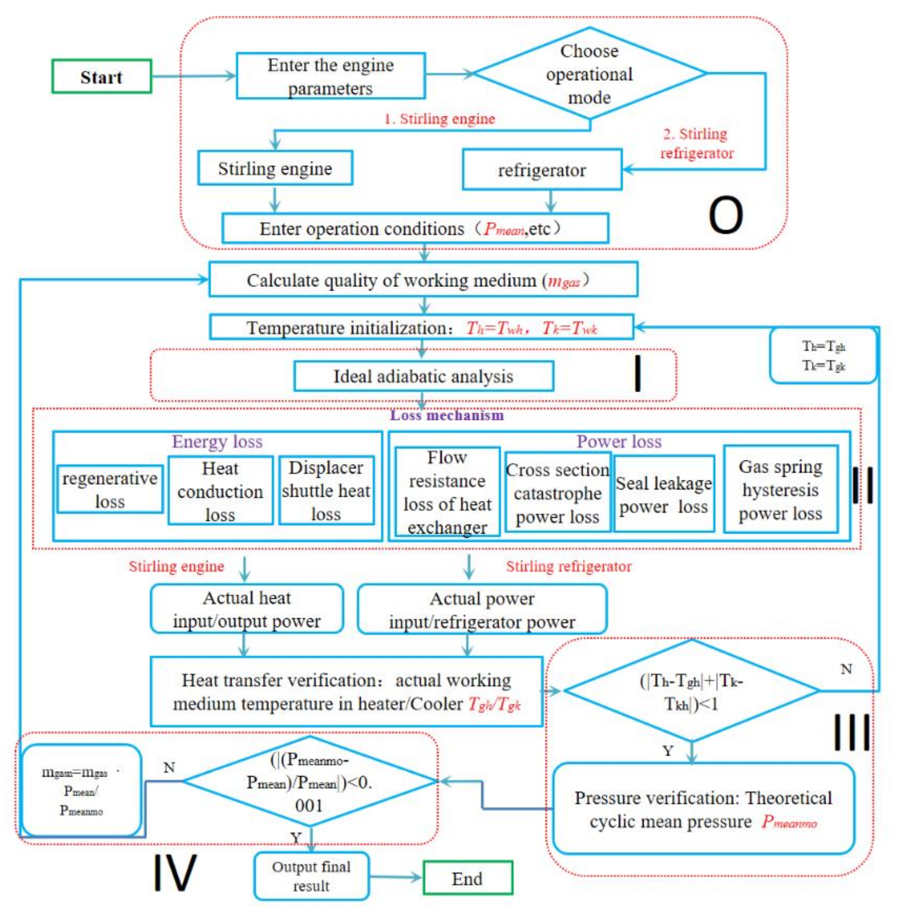
2.1. Improved Simple Model Combined with Various Heat and Power Losses

Figure 1 illustrates a schematic diagram for a framework of an improved Simple model combined with various heat and power losses, which was developed based on an ISAM model [26,27] and can be applied to Stirling engines and refrigerators simultaneously. The Stirling-cycle analysis model mainly consists of four parts: the adiabatic analysis module, the loss analysis module, and the temperature and pressure check modules. Based on an ideal adiabatic model, the power/heat losses of engine components and the actual heat-transfer processes are fully considered. The control equations of the adiabatic analysis model [4] are shown in Appendix A. The heat/power losses considered in the model mainly include the heat conduction loss, regenerative heat loss, displacer shuttle heat loss, flow resistance loss of the heat exchanger, cross-section mutation power loss, gas spring hysteresis power loss, and seal leakage power loss.

(1) Heat conduction loss: heat conduction through the engine body.

(2) Regenerative heat loss: the temperature difference between the fillers and gas cannot be neglected for an actual regenerator, indicating that more heat is needed for a thermal cycle.

(3) Shuttle heat loss of the displacer: the displacer brings some heat from the hot chamber into the cold one, which means the heater should absorb more heat.

(4) Flow resistance power loss of the heat exchanger: pressure drops in the heat exchangers, especially in the regenerator, reduce the final power output.

(5) Cross-section mutation power loss: the velocity direction and pressure distribution of the gas flow, due to the sudden expansion or contraction of the pipe section, which makes a drop in the output power.

(6) Gas spring hysteresis power loss: for an ideal gas, the pressure/volume relationship is either isothermal or adiabatic. For real gas, this imperfect thermodynamic process dissipates some work.

The corresponding calculation equations of these losses are shown in

Table 1. Heat and power losses in analytical model.

Category		Equation	Description
Heat losses	heat conduction loss (W) [28]	$Q_w=\frac{k_m{A}_w\Delta T}{l}$	Qw: heat conduction loss (W) km: material thermal conductivity (WK−3) Aw: cross-sectional area (m2) l: component length (m)
	regenerative heat loss (W) [29]	$Q_{rloss}=Q_r\left(1-\epsilon \right)$ $\epsilon =\frac{NTU}{1+NTU}$ $NTU=\frac{1}{2}St{A}_{wg}/A_r$ $St=0.46R{e}^{-0.4}P{r}^{-1}$	Qrloss: regenerative heat loss (W) Qr: heat transferred to the regenerator (W) ε: regenerator effectiveness St: Stanton number Awg: regenerator internal wetted area (m2) Ar: regenerator internal free-flow area (m2)
	displacer shuttle heat loss (W) [30]	$Q_{sh}=\frac{\pi }{6}\frac{S_p^2{k}_g\left(Th-Tk\right)D_{cy}^2}{\delta L_p}\left(\frac{1+\lambda }{1+{\lambda }^2}\right)$ $\lambda =1+\frac{k_g}{2\pi \delta }\left(\frac{L_{tc}}{k_{mc}}+\frac{L_{tp}}{k_{mp}}\right)$ $L_{tc}=2\pi \sqrt{\frac{2k_{mc}}{{\rho }_{mc}{C}_{pc}2\pi \omega }}$ $L_{tp}=2\pi \sqrt{\frac{2k_{mp}}{{\rho }_{mp}{C}_{pp}2\pi \omega }}$	Qsh: shuttle heat loss (W) Sp: displacer stroke (m) Kg: gas heat conductivity coefficient (Wm−1K−1) Lp: displacer length (m) δ: gap between displacer and cylinder wall (m) Lt: thermal wavelength (m) Ltc: thermal wavelength of cylinder wall (m) Ltp: thermal wavelength of displacer wall (m) Kmc: material thermal conductivity of cylinder (Wm−1K−1) kmp: material thermal conductivity of displacer (Wm−1K−1)
Power losses	flow resistance loss of heat exchanger (W) [31]	$\Delta p_r=-\frac{2C_{ref}{\mu }_g{\rho }_g{u}_{g}V}{A_0{d}^2}$ $W_{fr}={{\displaystyle \int }}_0^{2\pi }\left(\Delta p_r\frac{\partial V}{\partial \theta }\right)d\theta$	Wfr: flow resistance loss of heat exchanger (W) Cref: Reynolds friction factor V: void volume (m3) A0: cross-sectional (free flow) area (m2)
	cross-section mutation power loss (W) [28,32]	$h_j=1-{\frac{A_1}{A_2}}^2\cdot \frac{u_1^2}{2g}$ $\Delta p_j=1-{\frac{A_1}{A_2}}^2\cdot \frac{{\mu }_g{\rho }_g{u}_g}{2}$ $W_{fj}={{\displaystyle \int }}_0^{2\pi }\left(\Delta p_j\frac{\partial V}{\partial \theta }\right)d\theta$	hj: cross-sectional loss coefficient A1: small free flow area (m2) A2: large free flow area(m2)
	gas spring hysteresis power loss (W) [33]	$W_{gp}=\sqrt{\frac{1}{32}\omega {\gamma }^3\left(\gamma -1\right)T_w{P}_{mean}{k}_g}{(\frac{\Delta V}{V_B})}^2{A}_w$	Wgp: gas spring hysteresis power loss (W) γ: insulation factor Tw: average wall temperature (K) Pmean: average pressure (MPa) ΔV: volume amplitude (m3) VB: mean volume of the gap spring cavity (m3) Aw: mean wetted area (m2)
	seal leakage power loss (W) [33,34]	$W_{leak}=q_{leak}\cdot C_p\cdot T_{leak}$ $q_{mleak}=\rho \pi D_c\left(\frac{\Delta P{h}_0^3}{12\eta L}+\frac{u_p{h}_0}{2}\right)$	Wleak: seal leakage power loss (W) qmleak: leakage mass flow (kg·s−1) Tleak: leakage gas temperature (K) ΔP: pressure difference (MPa) Dc: cylinder diameter (m) h0: cylinder wall roughness up: piston velocity (ms−1) L: piston ring axial length (m)

. In the model, the actual mass of the working gas calculated by the Schmidt model was corrected, and the change of the physical parameters of the gas and the change of pressure and temperature were coupled. The convergence criterion is achieved when the temperature error is less than 1 °C and the relative error of the pressure is less than 0.1%. The smaller values (such as 0.1 °C and 0.01%) were adopted, and the convergence results were almost the same when calculating the convergence results. The above values (1 °C and 0.1%) were adopted in order to save calculation time.

As for the positive cycle, power losses directly affect the engine power whilst heat losses affect its ability to absorb heat directly, impacting the working gas temperature of the compression/expansion space and the cycle efficiency of the engine. However, for the reverse cycle, the power losses directly affect the input power, with heat losses affecting the actual cooling power of a cold head. This will also affect the temperature of the working gas and COP. The heat absorption/cooling capacity and cycle power equations of positive and reverse can be expressed as follows.

For the positive cycle:

$$Q_{ach}=Q_{adh}+Q_w+Q_{rloss}+Q_{sh}$$

(1)

$$Q_{acco}=Q_{adco}+Q_w+Q_{rloss}+Q_{sh}+W_{fr}+W_{fj}+W_{gp}+W_{leak}$$

(2)

$$W_{acipo}=W_{adip}-W_{fr}-W_{fj}-W_{gp}-W_{leak}$$

(3)

While for the reverse cycle:

$$Q_{acc}=Q_{adh}-Q_w-Q_{rloss}-Q_{sh}$$

(4)

$$Q_{acco}=Q_{adco}+Q_w+Q_{rloss}+Q_{sh}+W_{fr}+W_{fj}+W_{gp}+W_{leak}$$

(5)

$$W_{acipi}=W_{adip}-W_{fr}-W_{fj}-W_{gp}-W_{leak}$$

(6)

The heat transfer process is implemented to obtain the actual gas temperature in the hot/cold ends.

$$T_{ge}=T_{wh}-\frac{Q_{acc}}{h_{Ah}}$$

(7)

$$T_{gc}=T_{wk}-Q_{acco}/h_{Aco}$$

(8)

$$h=Nu·\lambda /d$$

(9)

$$Nu=0.023·Re·0.8·P{r}^n \left(heat: n=0.4, cool: n=0.3\right)$$

(10)

where Q_ach is the actual heat input (W) of SE; Q_adh is the adiabatic analysis heat input (W); Q_acco is the actual cooling power (W); Q_adco is the adiabatic analysis cooling power (W); W_acipo is the actual cycle power (W) of SE; W_adip is the adiabatic analysis cycle power (W); T_ge/T_gc is the working gas temperature in the expansion/compression space (°C); T_wh/T_wk is the heater (heat absorber)/cooler wall temperature (°C); A_h/A_co is the heater (heat absorber)/cooler convection heat transfer area (m²); Q_acc is the actual cooling power of SR (W); W_acipi is the actual cycle input power (W) of SR; Q_w is the heat conduction loss (W); Q_rloss is the regenerative heat loss (W); Q_sh is the displacer shuttle heat loss (W); W_fr is the flow resistance loss of the heat exchanger (W); W_fj is the cross-section mutation power loss (W); W_gp is the gas spring hysteresis power loss (W); and W_leak is the seal leakage power loss (W).

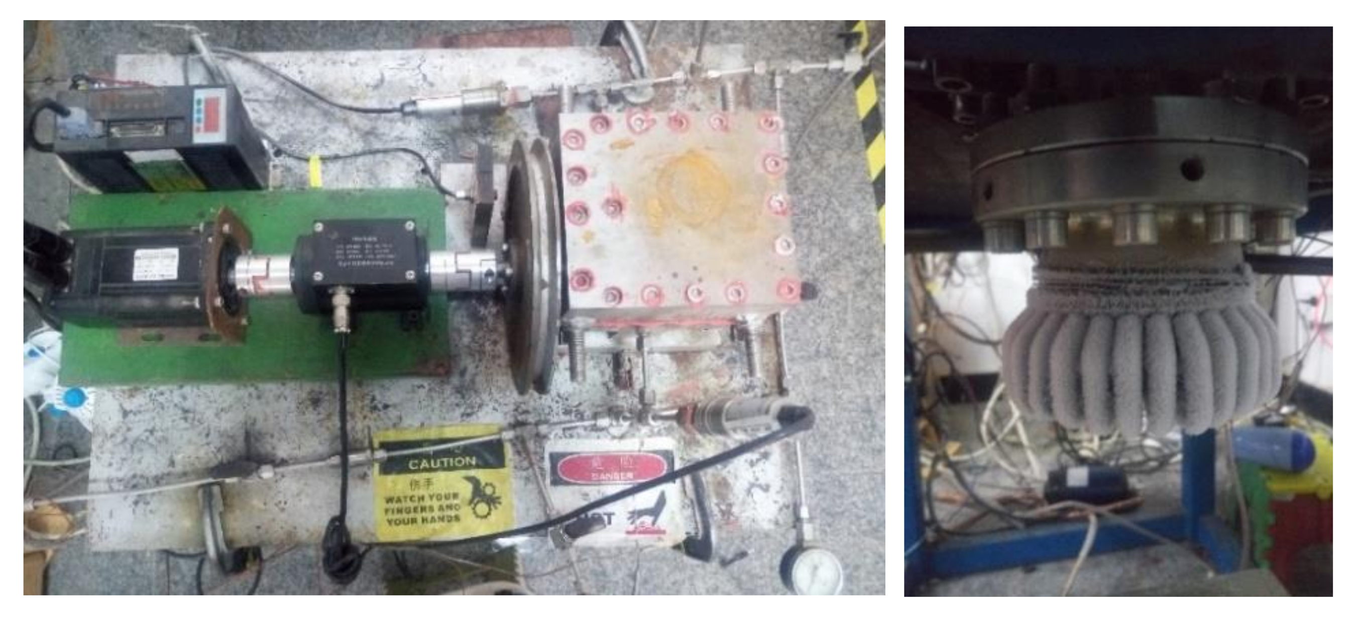
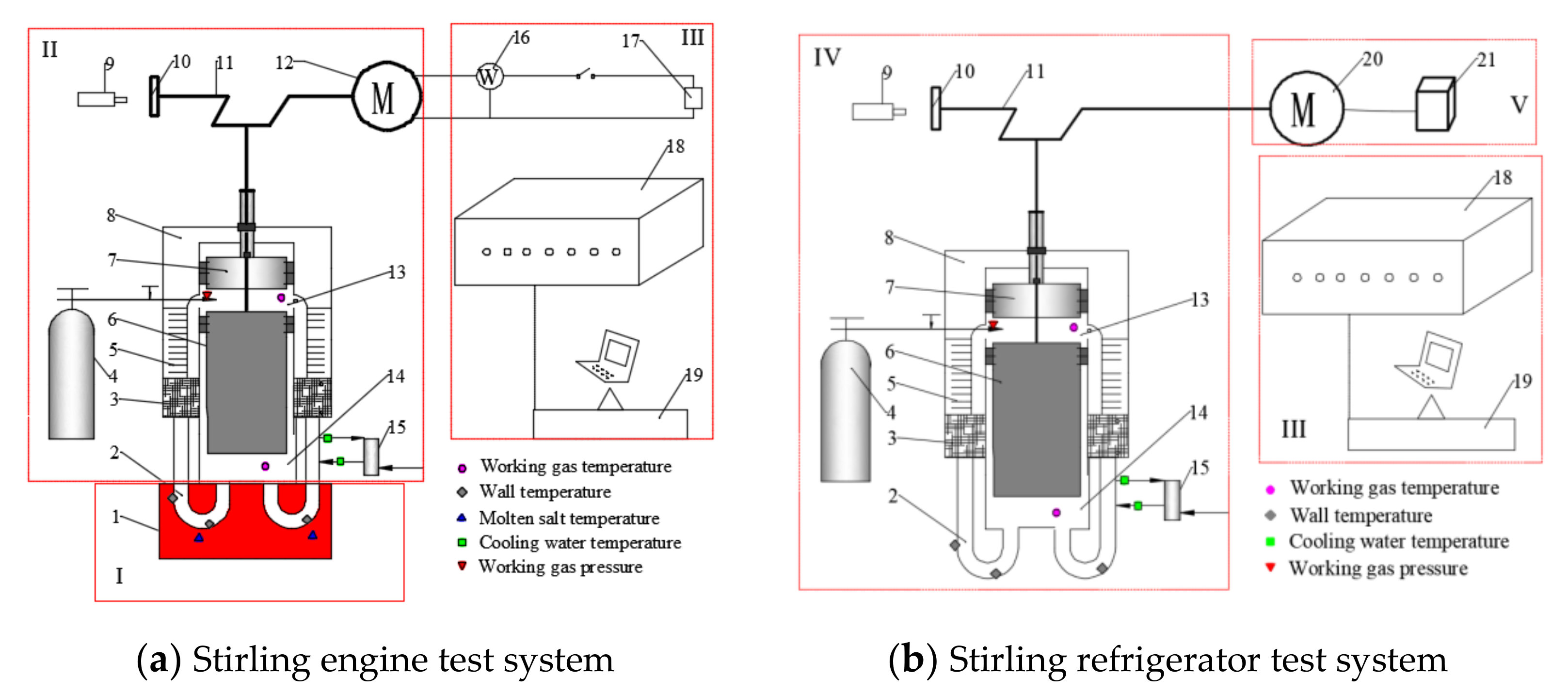
2.2. Experimental System

The performance of the Stirling engine and the refrigerator was studied to verify the accuracy and applicability of the improved Simple model. The three-dimensional structure of the engine and the measuring point arrangement are shown in Appendix A, with detailed parameters of the Stirling engine and the measuring instruments. Figure 2 shows the Stirling engine and the refrigerator-performance test system, consisting of three parts: a salt bath heating system, a β-type Stirling engine, and a data acquisition system [26]. The Stirling engine was heated by a salt bath whose temperature was maintained at 535 °C ± 2 °C. The internal working gas of a Stirling engine experiences a Stirling cycle, and the outputs work externally, driving a generator to create electricity. The Stirling refrigerator-performance test system also included three main parts: a servo motor, a refrigerator, and a data acquisition system. The measuring points of the Stirling engine and the refrigerator mainly included the gas temperature in the expansion/compression space, the gas pressure in the compression space, the temperature of the cooling water, the engine speed, and the crank angle of the flywheel.

3. Verification of the Model with GPU-3 Stirling Engine

The model was validated and analyzed by taking the GPU-3 Stirling engine, which was developed by General Motors [2,4], as a case. Some second-order analysis models [4,5,7,26,30] produced good results and exhibited good agreement with the experimental data when compared with the original Simple model proposed by Urieli and Berchowitz [4]. Timoumi’s team [30] considered five kinds of energy losses, i.e., regenerator heat transfer loss, shuttle heat loss, flow resistance loss, gas spring hysteresis loss, and heat conduction loss. The finite speed thermodynamics principles were incorporated in the CAFS model [7]. The quasi-steady flow approach was adopted to analyze the heat-transfer and flow-friction effects of the heater, cooler, and regenerator on the performance of the engine in Fawad’s optimization model [5].

Table 2. Comparison of different models’ results with experimental data of the GPU-3 Stirling engine.

Type of model	Cycle Power (W)	Error of Cycle Power	Cycle Efficiency (%)	Error of Cycle Efficiency
Experiment [2]	3958		35
Adiabatic model (Urieli and Berchowitz [4])	8300	109.7%	62.5	78.6%
Simple model (Urieli and Berchowitz [4])	6700	69.3%	52.5	50.0%
Dynamic best model (Timoumi [30])	4273	8.3%	38.49	10.0%
CAFS model (Hosseinzade [7])	4107	3.8%	36.2	3.4%
Fawad’s optimization model [5]	4507	13.9%	36.56	4.5%
Improved Simple analysis model in this paper	4256	7.5%	35.3	0.9%

shows the model results compared with those of some previous methods under rated conditions (a heat source temperature of 977 K, a heat sink temperature of 288 K, an average pressure of 4.14 MPa, a rotational speed of 2500 r/min, and a total mass of working gas of 1.1362 g). Compared with the ISAM model [23], the cycle’s average pressure was corrected, and the accuracy was greatly improved with the average pressure reduced from 4.26 MPa to 4.14 MPa and the mass from 1.255 g to 1.137 g.

The model has a good applicability with a wide operating range. Figure 3 and Figure 4 compare the indicated power and the cycle efficiency between the model values and the experimental ones of the GPU-3 Stirling engine when working at different conditions. The indicated power for H₂ increases, while the cycle efficiency increases at first and then decreases with the rise of rotational speed. The optimal rotational speed of H₂ is around 1500–2500 r/min. In general, the greater the pressure, the greater the corresponding indicated power and cycle efficiency. As to He, the indicated power increases at first and then gradually decreases with the increasing of the rotational speed, while the cycle efficiency shows an overall downward trend. This is due to the sharp increase in the flow resistance loss of the heat exchanger and the cross-section mutation power loss as the rotational speed increases. Indicatively, the predicted errors of the power and cycle efficiency are within 12% and 14%, respectively, when the rotational speed is in a range of 1000–3500 r/min with the H₂ at a constant pressure of 1.38 MPa and 2.76 MPa. The predicted errors of the indicated power and cycle efficiency are within 9% and 13%, respectively.

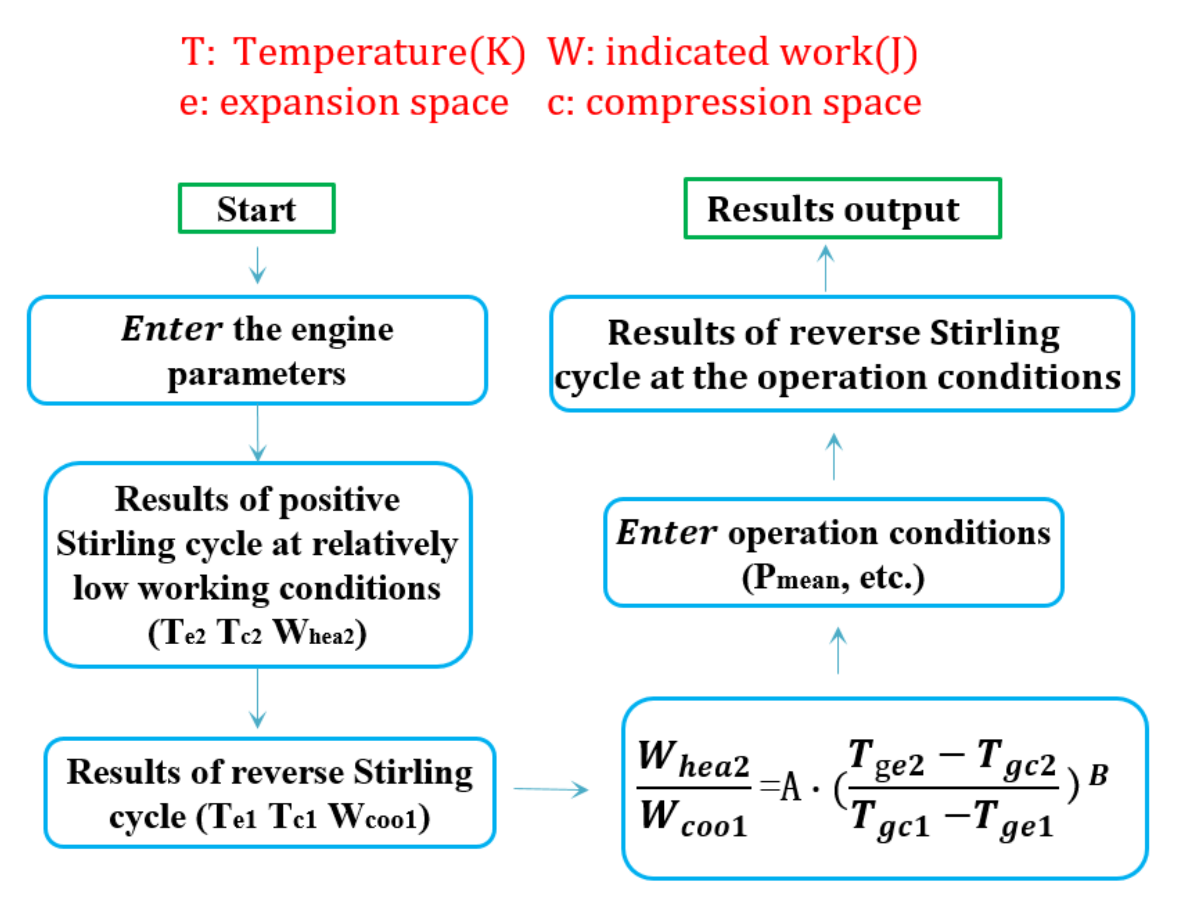
4. A Method to Predict the Performance of Positive Stirling Cycles Based on Reverse Stirling Cycles

The Stirling cycle, which consists of two isothermal processes and two isochoric processes, can be used as a prime mover, a refrigerator, and a heat pump depending on the direction of the cycle and the difference in the temperature of the hot and cold end. When used as the prime mover, the Stirling cycle goes along the clockwise direction and absorbs heat at a higher temperature. When used as a refrigerator, the direction of cycle is exactly the opposite. The refrigerator is driven by a motor and requires an external input of electric energy. Moreover, the cycle absorbs heat from the outside at a lower temperature.

Figure 5 shows the p-V map and the T-S map of the ideal Stirling cycle, showing the cycle direction and temperature domain of the ideal Stirling cycle. The 1-2-3-4-1 positive cycle is the prime-mover cycle, and the 1-2-3’-4’-1 reverse cycle is the refrigerator cycle. Based on the ideal Stirling cycle, the positive and reverse cycles have the same compression work, but the expansion work of the positive cycle is much larger than the compression work, and the area of 1-2-3-4-1 is the indicated work of the Stirling engine. As to the refrigerator, the expansion work of the cycle is much smaller than the compression work, and the area of 1-2-3’-4’-1 is the indicated work input; that is the reason why the refrigerator needs a motor to drag. According to the ideal Stirling-cycle map, the cycle thermal efficiency of the prime-mover cycle and the coefficient of the performance of the refrigerator are shown in Equations (11) and (12), respectively. The efficiency of the Stirling cycle is the same as that of the Carnot cycle at the same temperature.

$${\mathsf{\eta }}_C=\frac{\mathrm{Cycle}\mathrm{power}\left(\mathrm{W}\right)}{Absorbed heat ({\mathrm{Q}}_E)}=1-\frac{T_C}{T_E}$$

(11)

$${\mathrm{COP}}_{ref}=\frac{Absorbed heat ({\mathrm{Q}}_E)}{\mathrm{Cycle}\mathrm{power}\left(\mathrm{W}\right)}=\frac{T_{ref}}{T_C-T_{ref}}$$

(12)

where ${\mathsf{\eta }}_C$ is the cycle thermal efficiency of the Stirling engine, ${\mathrm{COP}}_{ref}$ is the coefficient of the performance of the Stirling refrigerator, T_C is the temperature of the gas in the compression space, T_E is the temperature of the gas in the expansion space, and T_ref is the refrigerator temperature.

The internal working gas of the Stirling engine carries on the complex oscillating flow-heat and mass-transfer process, and in the applicability and accuracy of the Stirling cycle model similar problems also exist. Some problems of the performance evaluation of the Stirling engine caused by testing difficulties can be solved if the indicated work of the Stirling refrigerator can be used to predict the Stirling positive-cycle results. Figure 6 is the logic graph of the method to predict the performance of the positive Stirling cycles based on the reverse ones. The method mainly includes three parts:

I.

Carry out the positive and reverse Stirling cycles at the same low conditions according to the same Stirling engine working as both a prime mover and a refrigerator.

II.

Establish a mathematical model based on the positive and reverse Stirling cycles in part I.

III.

Carry out reverse Stirling cycles at high conditions and predict the performance of the positive Stirling cycles based on the mathematical model in part II.

Specifically, the Stirling positive- and reverse-cycle experiments were carried out under the same low conditions (mean pressure and rotational speed) to obtain the upper and lower temperature limits of the Stirling cycle, including the gas temperature of the expansion and compression space as well as the cyclic p-V diagram, which can be used to calculate the indicated work. The most important part is to use mathematical models to establish the relationship between the work of the positive and reverse Stirling cycles. The mathematical model to predict the indicated power is shown in Equation (13). The difference between the cycle works of the positive and the reverse Stirling cycles is mainly affected by the cycle temperature difference in the case of controlling the same mean pressure and the rotational speed. Equation (13) is used to establish a dimensionless parameter based on temperature difference.

$$\frac{W_{heat2}}{-W_{cool1}}=\mathrm{A}·{(\frac{T_{ge2}-T_{gc2}}{T_{gc1}-T_{ge1}})}^B$$

(13)

where W_heat2/W_cool1 is the cycle power (W) of the positive/reverse Stirling cycle, T_ge2/T_gc2 is the gas temperature in the expansion/compression space for the positive Stirling cycle, and T_ge1/T_gc1 is the gas temperature (K) in the expansion/compression space for the reverse Stirling cycle, where A is the pressure term coefficient, related to the pressure. When A < 1, the control pressures of the positive/reverse Stirling cycles are equal, and the average temperature of the reverse Stirling cycle is lower, which means that the mass of corresponding working fluid is larger. B is the temperature term coefficient, which is assumed to be unchanged for the same Stirling engine. The Stirling engine cycle power results under the needed conditions are predicted by performing a refrigeration cycle under the required operating conditions and the indicated work relationship model.

5. Results and Discussion

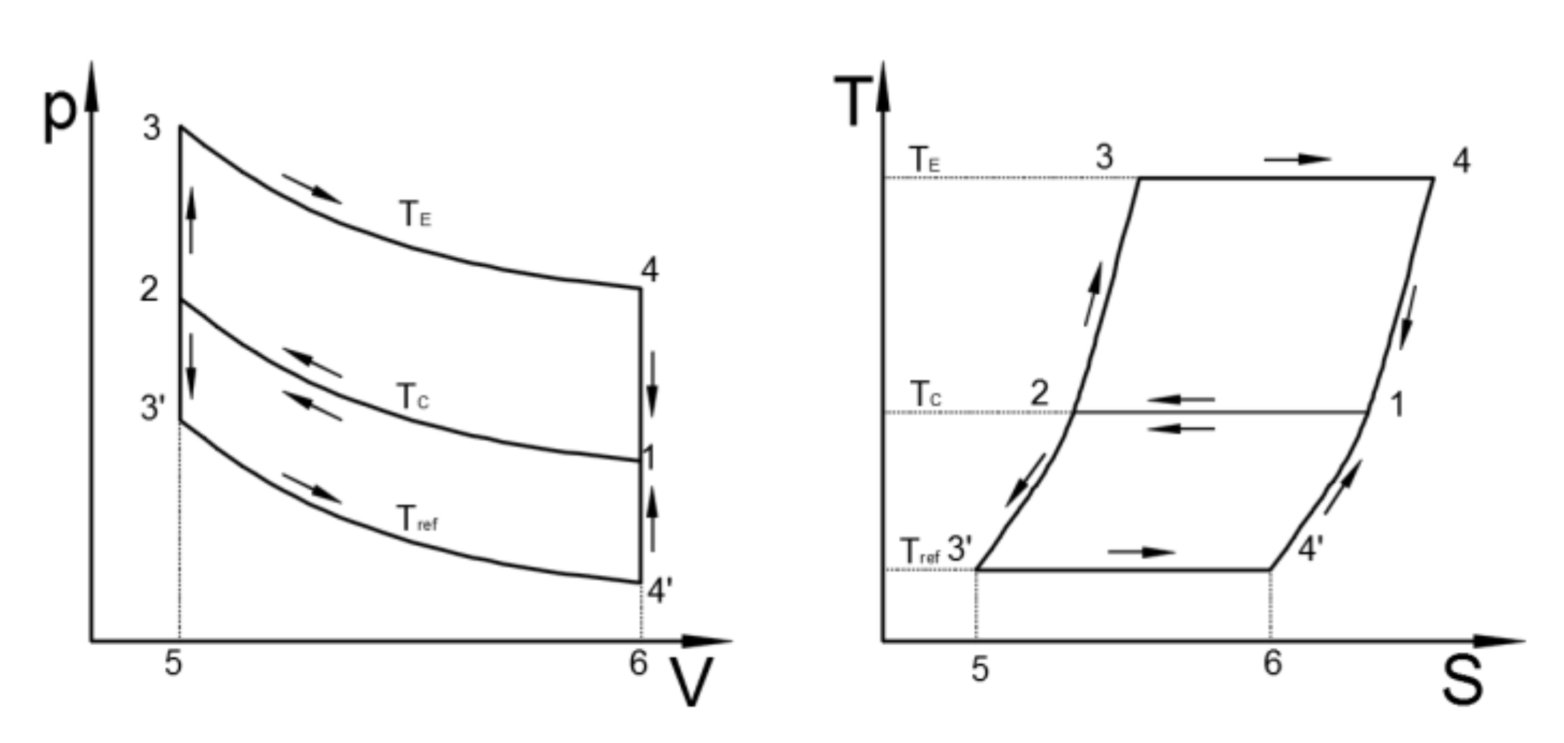
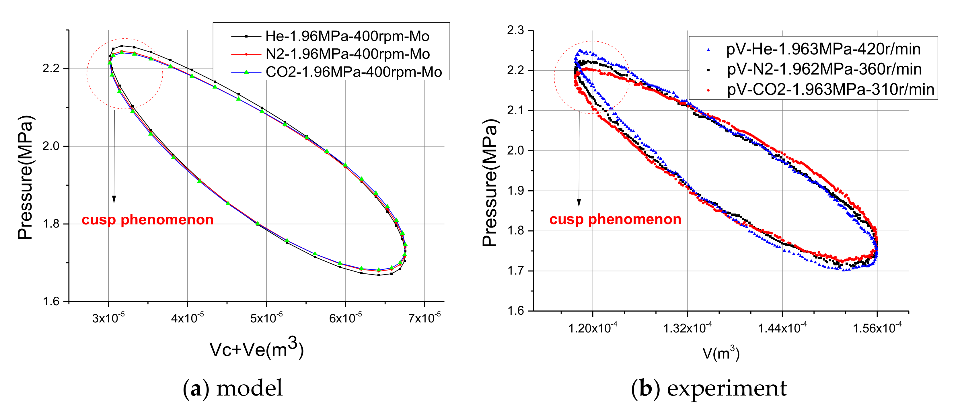
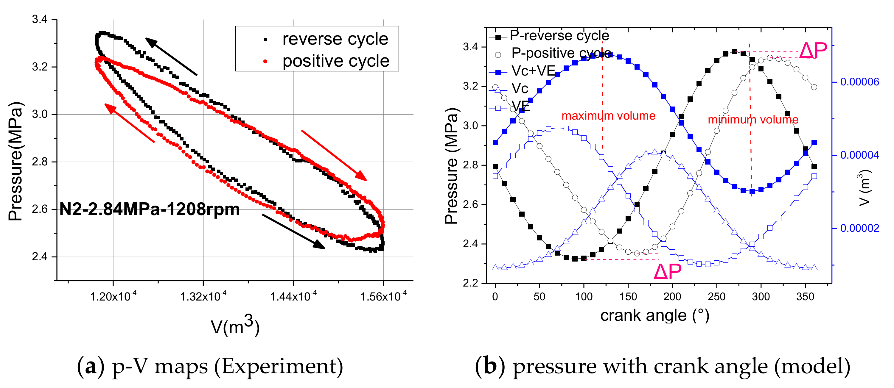
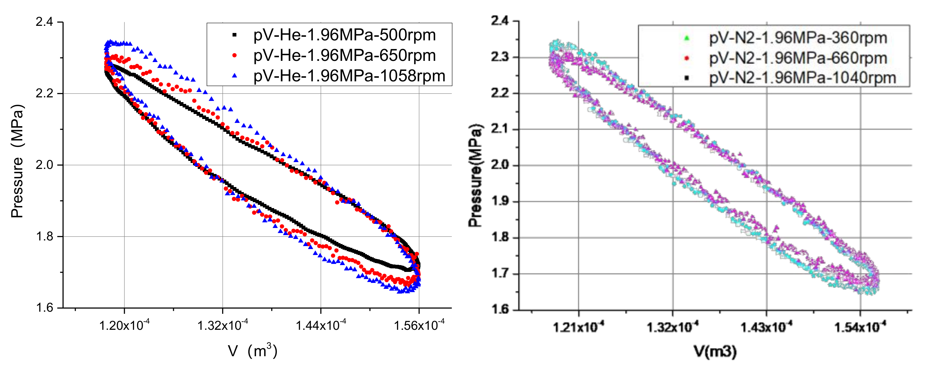
5.1. Positive and Reverse Stirling Cycles’ p-V Maps

As shown in Figure 7a, there is a “cusp phenomenon” in the p-V map obtained by the ideal adiabatic model, which is more remarkable in the experimental results (Figure 7b). The “cusp phenomenon” refers to the fact that the minimum volume part of the p-V map is sharper than the maximum volume part. Figure 8 shows the variation between the total volume of the expansion and compression spaces with the crank angle. The change rate of the volume near the minimum volume point is greater than that near the maximum volume point, which contributes to the “cusp phenomenon”.

Figure 9a shows the p-V maps of the positive and reverse Stirling cycles at the same mean pressure. The distinction between the p-V maps is mainly reflected in the “pressure ratio” and “curve shape”. The pressure ratio of the reverse Stirling cycle is significantly higher than that of the positive one, and the p-V map of the Stirling engine is asymmetric, while relatively harmonious, for the refrigerator.

For the positive cycle, the expansion-space volume continues to increase while the compression-space volume decreases after the minimum volume point, and the temperature of the working gas increases overall; thus, the maximum pressure of the positive cycle is ahead of the minimum volume point. Similarly, the maximum pressure of the reverse cycle lags behind the minimum volume point, as shown in Figure 9b. The maximum pressure of the positive cycle is smaller than that of the reverse one, as shown in Figure 9b. In addition, the minimum pressure of the positive cycle is ahead of the minimum volume point; however, that of the reverse cycle lags behind the maximum volume point. The minimum pressure of the positive cycle is larger than that of the reverse one. The peak pressure occurs at the expansion progress for the positive cycle and the compression progress for the reverse cycle, while the trough pressure occurs at the compression progress for the positive cycle and the expansion progress for the reverse cycle. The effect of the minor loss caused by the sudden change of the cross-section area and flow resistance loss on the positive cycle is more remarkable than on the reverse cycle, which is a possible reason for the obvious “higher pressure ratio” phenomenon of the reverse cycle.

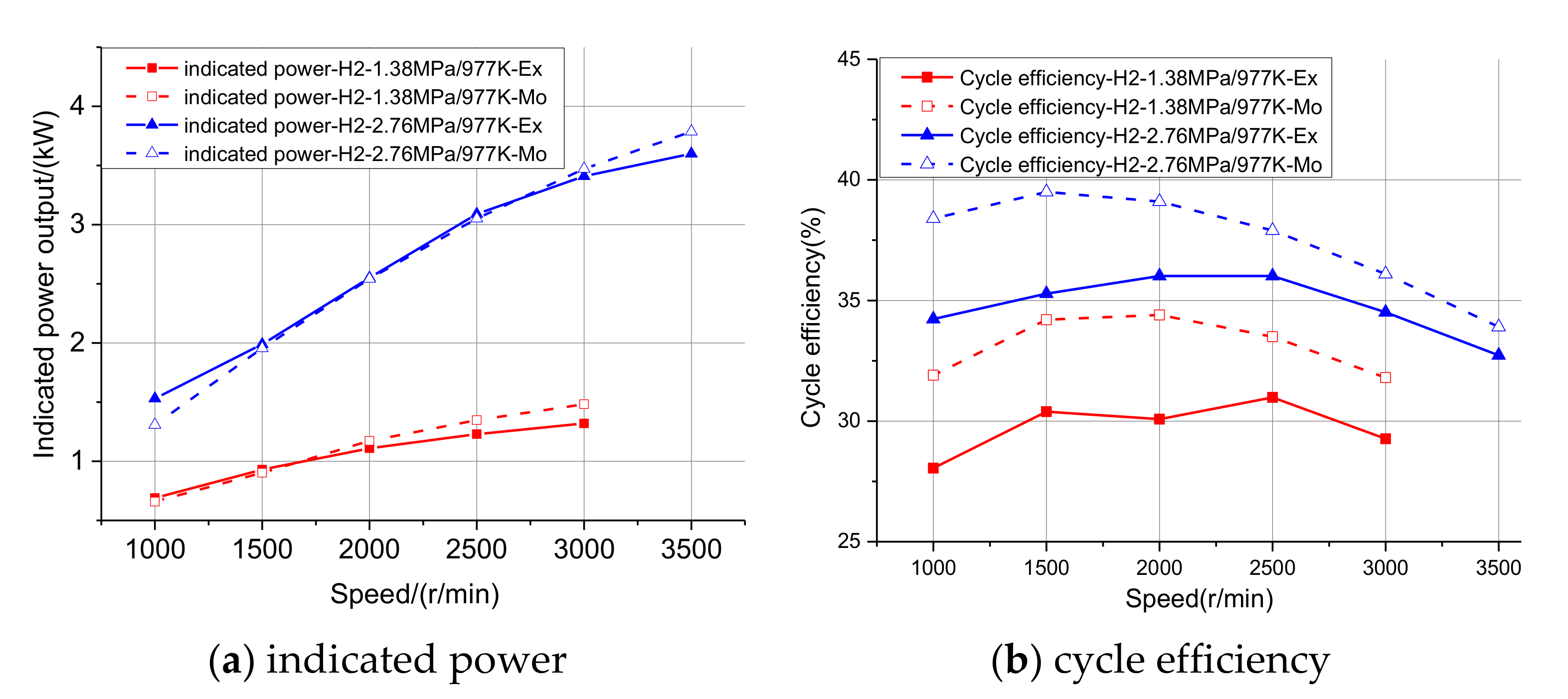
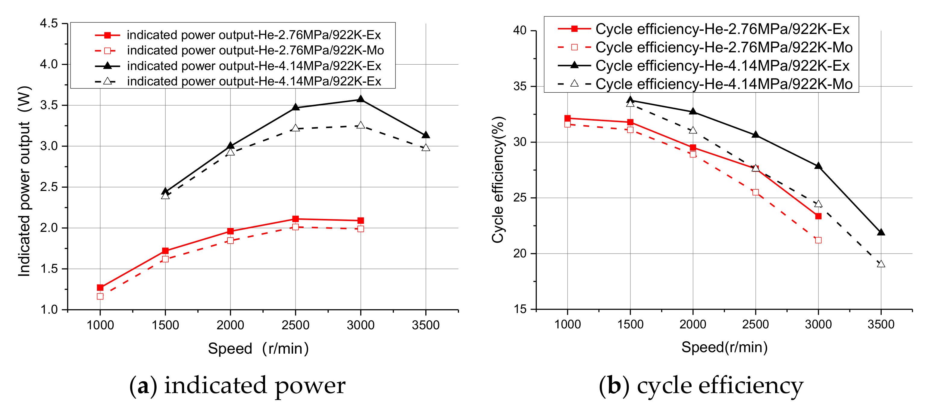
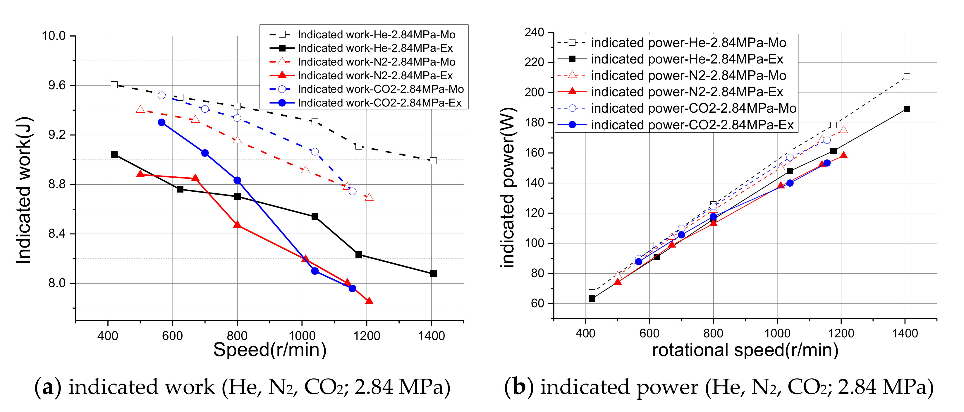
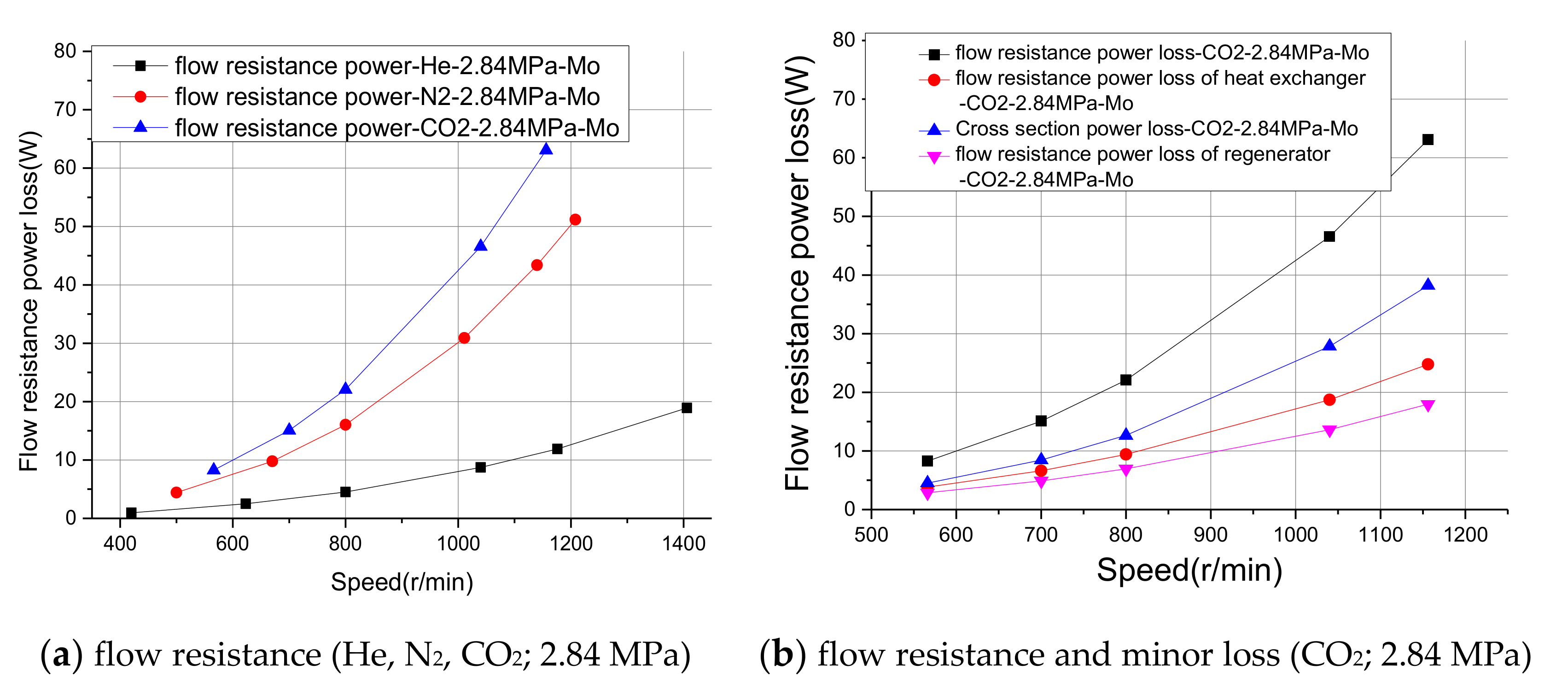
5.2. Performance of Stirling Engine

Figure 10a,b shows the changes in the indicated work and power with the rotational speeds at a constant pressure of 2.84 MPa. Both the model and the experimental results demonstrate that the indicated work gradually decreases while the indicated power increases, with a relative error range of 6.2–11.3%, as the rotational speed increases with He.

Figure 10c shows that the cycle efficiency for He increases with the rotational speed, while the slope of the increase gradually slows down. However, the cycle efficiency for N₂ and CO₂ increases at first and then decreases, indicating that there is an optimal rotational speed for a certain pressure. The value of the optimal rotational speed is ordered as He > N₂ > CO₂ and decreases with the increasing pressure, as shown in Figure 10d. The flow resistance loss of the heat exchangers and the regenerative heat loss of the regenerator increases sharply as the rotational speed increases, resulting in a decrease for the indicated power and a dramatic increase in the heat-absorption rate. The model’s predicted errors are within 10.2%, 7.5%, and 13.7% for the He, N₂, and CO₂, respectively.

The indicated work and cycle efficiency are mainly influenced by temperature ratio, pressure ratio, regenerative heat loss, flow resistance loss, and minor loss. The leakage loss is independent whilst the flow resistance loss increases exponentially along with the increase in the rotational speed, as shown in Figure 11; thus, the cycle power increases slowly and even decreases. The total flow resistance loss increases from 1.0 W to 18.9 W, from 4.42 W to 51.2 W, and from 8.26 to 63.1 W for the He, N₂, and CO₂ at 2.84 MPa, respectively. The flow resistance for CO₂ is larger than that for He and N₂, and the difference is more noticeable with the increase in rotational speed. The regenerator is the largest flow-resistant component in the Stirling engine and has a great influence on the cycle efficiency. About 50% of the power and heat losses are related to the regenerator [35]. Gheith et al. [36] proposed that the regenerator is a key component of the Stirling engines. Furthermore, the flow asymmetry should be considered for a deep analysis of the internal flow and temperature fields. The researcher put much focus on the inner structure of a regenerator, filling porosity, or material [37,38]. Here, we focus on the internal heat and mass transfer with different working gases, as shown in

Table 3. Stirling engine operating characteristics of different working gases.

Experimental Value	Mean Pressure (MPa)	Speed (r/min)	Cycle Power (W)	Cycle Efficiency (%)	Indicated Work (J)	Shaft Power (W)	Electric Power (W)	Pressure Difference (MPa)	tge (°C)	tgc (°C)
He	2.84	1040	148.02	13.98	8.54	82.65	51	0.77	469	53.8
N2	2.84	1011	138.06	12.08	8.19	53.5	24	0.73	472.2	48.2
CO2	2.84	1040	140	11.26	8.1	46.37	12	0.71	473.9	40.7
Numerical Value	Cycle Power (W)	Indicated Work (J)	Cycle Efficiency (%)	Heat Conduction Loss (W)	Regenerative Heat Loss (W)	Shuttle Heat Loss (W)	Flow Resistance Loss (W)	Leakage Loss (W)	Spring Hysteresis Loss (W)	Flow Resistance Loss of Regenerator (W)
He	161.34	9.31	15.22	407.5	41.6	62.5	8.7	42.4	4	5.3
N2	150.17	8.91	12.53	407.1	132.5	10.8	30.9	27.4	1	10.6
CO2	157.1	9.06	12.96	407.3	182.4	11.4	46.6	16.6	0.9	13.6

.

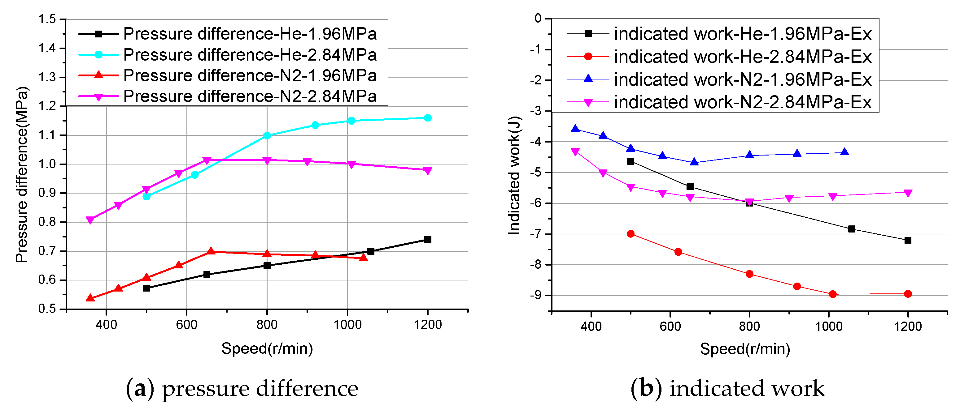
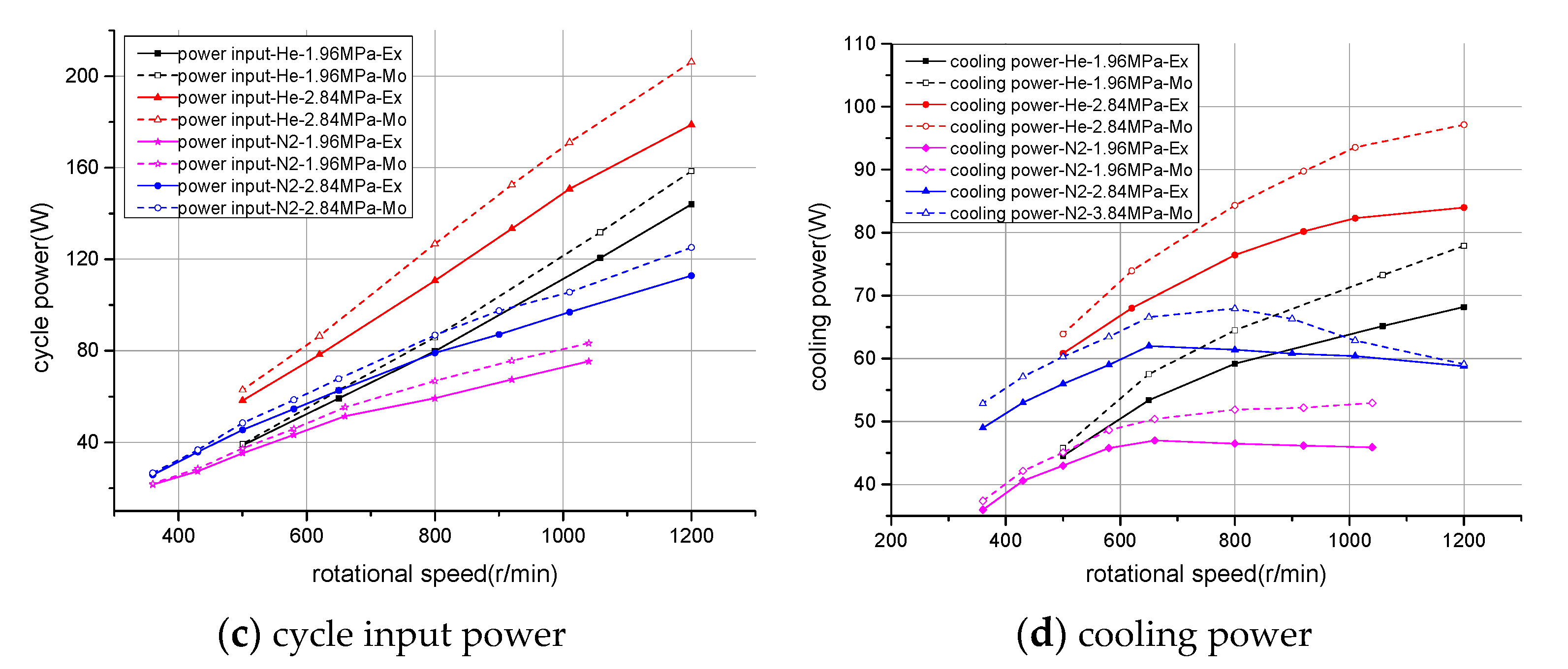
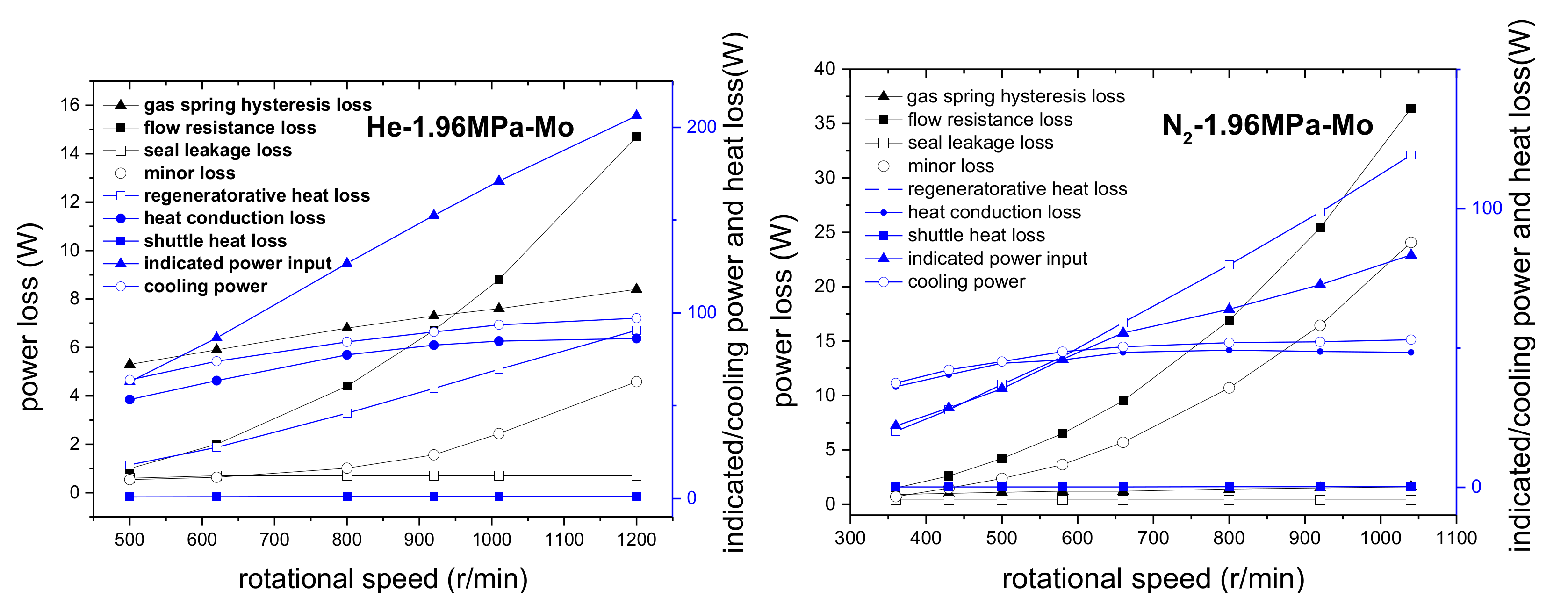
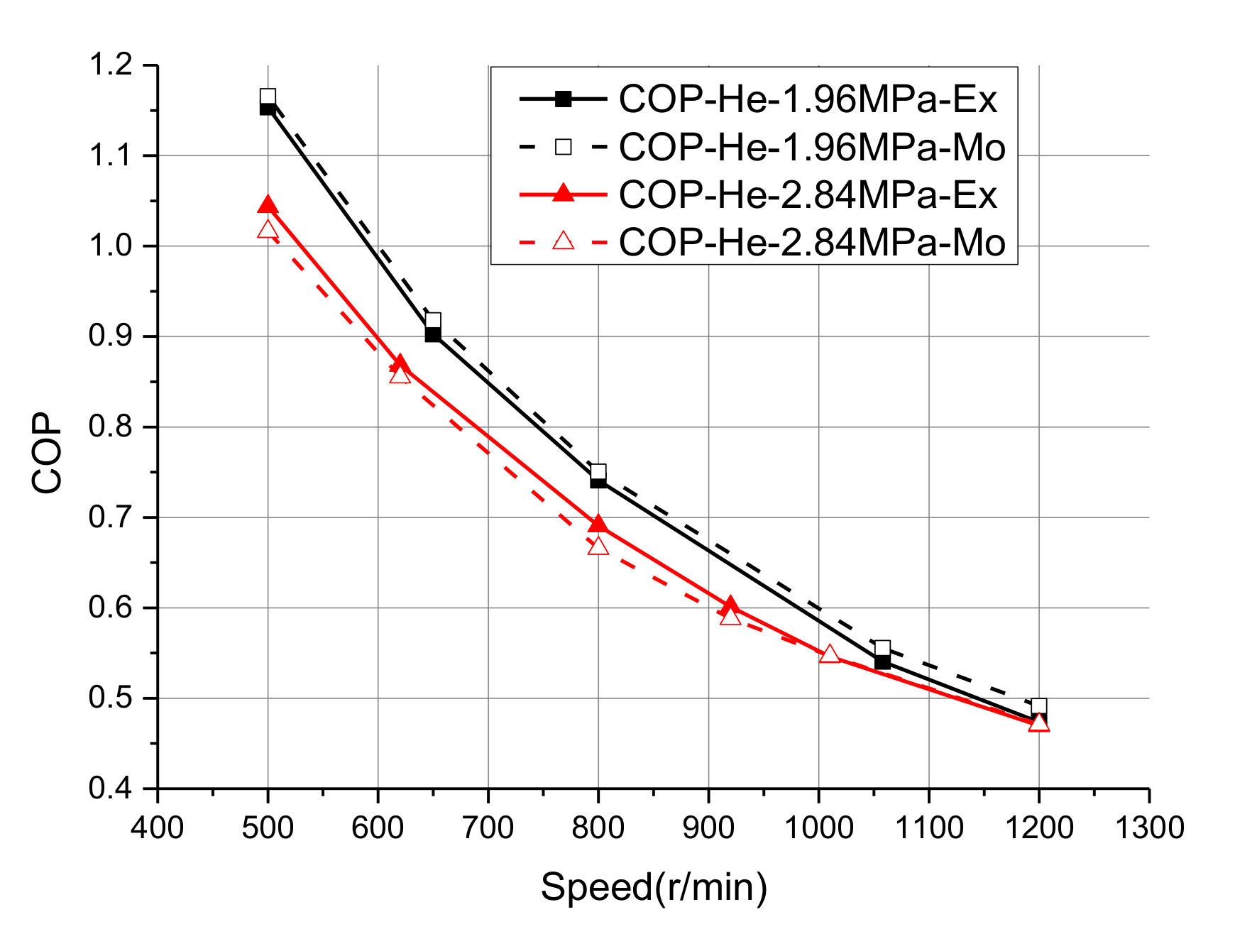
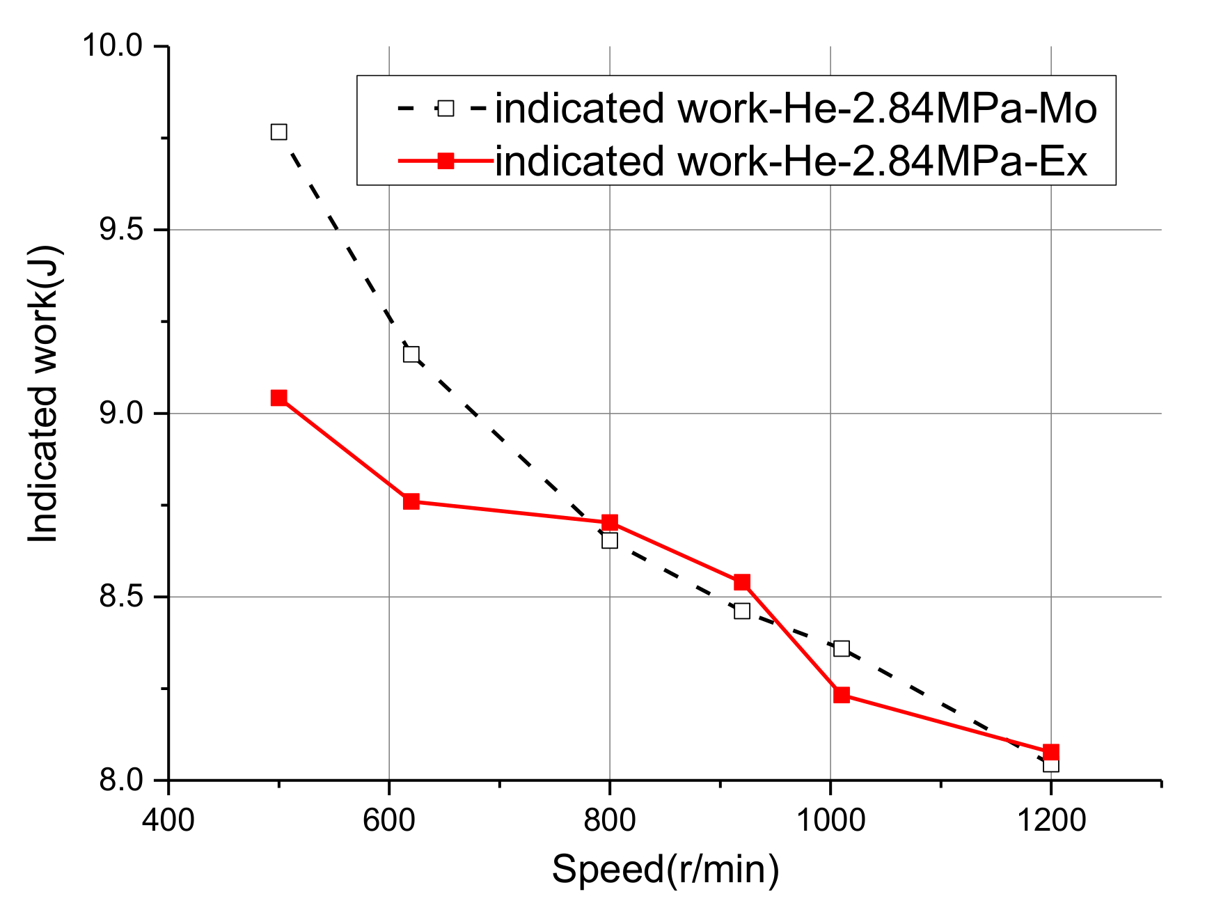
5.3. Performance of Stirling Refrigerator

The gas temperature of the expansion space reaches a relatively stable state after a certain period when the Stirling engine is connected with a servo motor. Both the model and the experimental results show that the cooling temperature for He decreases as the rotational speed increases, while the cooling temperature for N₂ decreases at first and then maintains a flat level with even a slight increase, as shown in Figure 12. The minimum cooling temperatures for He are smaller than those for N₂ at same mean pressures. The minimum cooling temperatures are −92.2 °C and −53.6 °C for He and N₂ at 2.84 MPa, respectively. The regenerative heat loss of He is much smaller than that of N₂, which leads to a significant decrease in the cooling power of N₂. Furthermore, there is an optimal rotational speed for the minimum cooling temperature, which is related to the type of working gases and pressures. It can be seen from Figure 12a that the optimal rotational speed for He is higher than that for N₂ and decreases as the mean pressure increases, as shown in Figure 12b. In addition, the cooling temperatures for He and N₂ are similar at lower rotational speeds (500 r/min), and the cooling temperature for He is lower compared with that of N₂ at higher rotational speeds, which indicates that He and other small molecule refrigerants have a greater refrigeration capacity in the Stirling refrigerator. Figure 13 shows the temperature variation of the gas in the compression space and the wall of cold head at different rotational speeds. The mass-flow rate increases as the rotational speed increases, resulting in an overall increase in the heat-exchange rate, and the temperature of the working gas in the compression space also increases. The minimum wall temperatures of the cold head are −87.2 °C and −46.1 °C for He and N₂, respectively.

It can be found from Figure 14 that the pressure ratio of the p-V map for He increases with the rotational speed, while for the N₂ it is almost invariant, which is closely related to the temperature ratio. The pressure difference for the He increases with an increase in the rotational speed, while that for the N₂ increases first and then decreases, as shown in Figure 15a. The indicated work reduces from −4.64 J to −7.20 J, and the cycle input power increases from 38.6 W to 144.0 W for He when the rotational speed increases from 500 to 1200 r/min at 1.96 MPa, as shown in Figure 15b,c, while for the N₂, it reduces from −3.59 J to −4.68 J (660 r/min) and then increases to −4.35 J when the rotational speed increases from 360 to 1200 r/min at 1.96 MPa. The cooling power for the He increases when the rotational speed increases, while the cooling power for the N₂ increases at first but then gradually decreases, as shown in Figure 15d. The predicted errors of the cycle input power and cooling power are within 10.9% and 14.5%, respectively, for the He and N₂ at different mean pressures.

The decrease in cooling power is mainly caused by an increase in heat conduction loss and regenerative heat loss. Figure 16 shows the variation of the cycle input power and the heat/power losses in the model at different rotational speeds. With the increasing of the rotational speed, the displacer shuttle heat loss is practically unchanged, while the heat conduction loss and the regenerative heat loss increase significantly. The regenerative heat loss for N₂ is greater for a lower thermal conductivity and a higher heat capacity compared with that of He. This indicates that the performance of the Stirling refrigerator is worse for N₂ at a high rotational speed. The COP coefficient (defined as: COP = $\frac{\mathrm{cold}\mathrm{head}\mathrm{cooling}\mathrm{power}}{\mathrm{cycle}\mathrm{input}\mathrm{power}})$ gradually decreases with the rotational speeds with a relative error of <4.5%, as shown in Figure 17, which is a combined result of an increase in the cycle input power and an overall decrease in the cooling power.

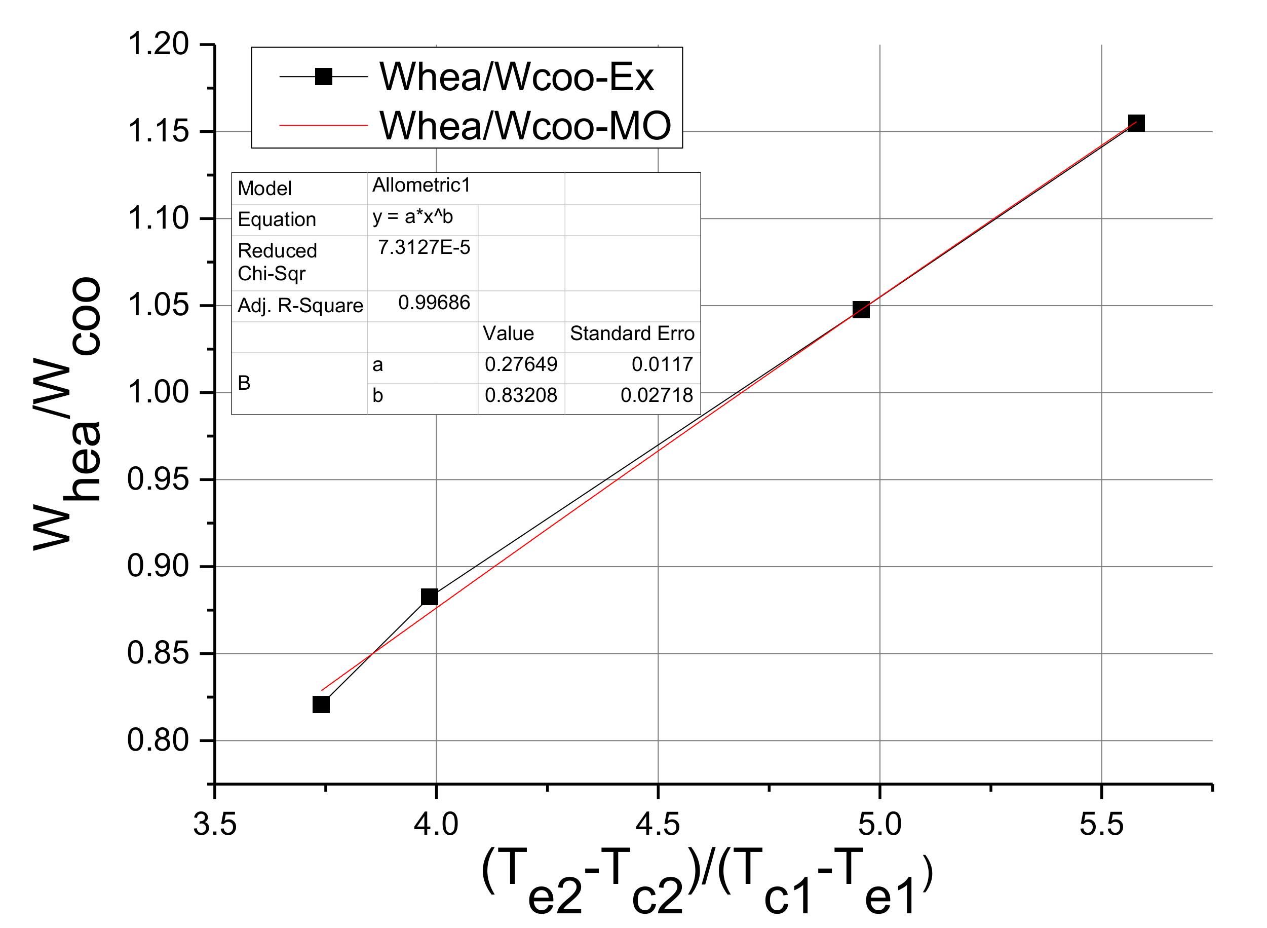
5.4. Relationship between the Indicated Work of Stirling Engine and Refrigerator of the 100 W Stirling Engine

The partial experimental results of the Stirling engines and refrigerators at 1.96 MPa and 800 r/min are listed in

Table 4. Stirling engines and refrigerators results with rotational speed (1.96 MPa, He).

Working Gas	Mean Pressure (MPa)	Speed (r/min)	Tc-Co (K)	Te-Co (K)	Indicated Work-Coo (J)	Cycle Power-Coo (W)	Te-He (K)	Tc-He (K)	Indicated Work-He (J)	Cycle Power-He (W)
He	1.96	650	299.30	222.11	5.46	59.19	746.39	315.74	6.31	68.35
He	1.96	800	301.02	214.73	5.99	79.89	746.42	318.62	6.28	83.69
He	1.96	1058	304.26	198.33	6.84	120.55	744.32	322.20	6.03	106.50
He	1.96	1200	306.50	194.20	7.20	144.00	743.43	323.36	5.91	117.30

and

Table 5. Stirling engines and refrigerators results with mean pressure (800 r/min, He).

Working Gas	Mean Pressure (MPa)	Speed (r/min)	Tc-Co (K)	Te-Co (K)	Indicated Work-Coo (J)	Cycle Power-Coo (W)	Te-He (K)	Tc-He (K)	Indicated Work-He (J)	Cycle Power-He (W)
He	1.42	800	298.61	224.00	4.32	57.66	747.25	316.05	3.93	60.40
He	1.96	800	301.02	214.73	5.99	79.89	746.42	318.62	6.28	83.69
He	2.15	800	301.39	205.64	6.52	86.96	745.52	319.63	6.70	89.36
He	2.41	800	302.30	197.80	7.28	97.07	745.47	320.02	7.39	98.53
He	2.84	800	304.10	191.00	8.30	110.67	743.58	322.27	8.70	116.03

. According to the numerical model given by Equation (13), detailed relations between the cycle work of the 100 W beta-type Stirling engine and the refrigerator are obtained according to Figure 18, as shown in Equation (14).

$$\frac{W_{hea2}}{-W_{coo1}}=\mathrm{A}·{(\frac{T_{ge2}-T_{gc2}}{T_{gc1}-T_{ge1}})}^{0.8321}$$

(14)

Furthermore, combined with the characteristics under different pressures, the pressure coefficient A is obtained, referring to

Table 6. The relationship between the pressure factor coefficient A and the pressure (He).

Mean Pressure (MPa)	A
1.42	0.211
1.96	0.276
2.15	0.297
2.41	0.316
2.84	0.351

. The reason for the pressure coefficient A < 1 is due to the mass of the working gas difference on account of the difference of the temperature at the same mean pressure.

Figure 19 shows the experiment and model results for He at the constant pressure of 2.84 MPa. The error between the model and the experimental value is at the range of −0.5–7.4%. Based on the results of the reverse cycle, the cycle power of the Stirling engine is predicted relatively accurately (the cycle-power result error is the same as with the cycle-indicated work on account of the same rotational speed).

6. Conclusions

In order to develop a practical method to evaluate the performance of a Stirling engine by it running as a refrigerator, an improved Simple model was proposed at first for positive and reverse Stirling cycles simultaneously. A self-designed β-type Stirling engine was tested and the experimental results verified the good applicability and accuracy of the model. As to the positive Stirling cycles, the model errors of the indicated power and the cycle efficiency were within 11.3% and 13.7%, respectively. The indicated power maximum was 189.3 W, with a cycle efficiency of 14.7% at 1406 r/min for He. As to the reverse cycles, the predicted errors of the cycle input power and cooling power were within 10.9% and 14.5%, respectively. The experimental cooling temperatures could reach −92.2 °C and −53.6 °C, respectively, for He and N₂ at 2.8 MPa.

The p-V maps of the positive and reverse Stirling cycles were obtained at the same control pressures. The distinction between the positive and reverse Stirling cycles’ p-V maps was mainly reflected in the “pressure ratio”. The pressure ratio of the reverse cycle was higher than that of positive one at the same mean pressure. The peak pressure occurred at the expansion progress for the positive cycle and the compression progress for the reverse cycle, while the trough pressure occurred at the compression progress for the positive cycle and the expansion progress for the reverse cycle.

In addition, a method was proposed to predict the indicated work of the positive Stirling cycles based on the reverse ones. The most critical issue with this method was to establish an associated model of the gas temperatures in the expansion/compression space. A mathematical model to predict the indicated power of the positive and reverse Stirling cycles was proposed: $\frac{W_{heat2}}{-W_{cool1}}=\mathrm{A}·{(\frac{T_{ge2}-T_{gc2}}{T_{gc1}-T_{ge1}})}^B.$ The error between the values of the model and the experiment with He at 2.8 MPa was at the range of −0.5–7.4%. These results indicate that the model can provide much useful information for studying a Stirling engine and a refrigerator simultaneously and will probably bring a practical method for forecasting a positive cycle through a reverse one.

References

1. Awan, A.B.; Zubair, M.; Memon, Z.A.; Ghalleb, N.; Tlili, I. Comparative analysis of dish Stirling engine and photovoltaic technologies: Energy and economic perspective. Sustain. Energy Technol. Assess. 2021, 44, 101028. [Google Scholar]
2. William R, M.; Martini Engineering. Stirling engine design manual. 1983. Available online: https://ntrs.nasa.gov/api/citations/19830022057/downloads/19830022057.pdf (accessed on 25 October 2021).
3. Ferreira, A.C.; Silva, J.; Teixeira, S.; Carlos Teixeira, J.; Azucena Nebra, S. Assessment of the Stirling engine performance comparing two renewable energy sources: Solar energy and biomass. Renew. Energy 2020, 154, 581–597. [Google Scholar] [CrossRef]
4. Urieli, I.; David, M. Berchowitz, Stirling Cycle Engine Analysis; A Hilger: Hilger, MT, USA, 1984. [Google Scholar]
5. Ahmed, F.; Huang, H.L.; Khan, A.M. Numerical modeling and optimization of beta-type Stirling engine. Appl. Therm. Eng. 2019, 149, 385–400. [Google Scholar] [CrossRef]
6. Tlili, I. Finite time thermodynamic evaluation of endoreversible Stirling heat engine at maximum power conditions—ScienceDirect. Renew. Sustain. Energy Rev. 2012, 16, 2234–2241. [Google Scholar] [CrossRef]
7. Hosseinzade, H.; Sayyaadi, H. CAFS: The Combined Adiabatic-Finite Speed thermal model for simulation and optimization of Stirling engines. Energy Convers. Manag. 2015, 91, 32–53. [Google Scholar] [CrossRef]
8. Crowley, J.L. Standardized efficiency terms: Comparison of some Stirling engine performance figures. In Proceedings Intersociety Energy Conversion Engineering Conference; Engineering Technology Division, Oak Ridge National Laboratory: Oak Ridge, TN, USA, 1984; Volume 3. Available online: https://www.osti.gov/biblio/5854341 (accessed on 25 October 2021).
9. Stine, W.B.; Diver, R.B. A Compendium of Solar Dish/Stirling Technology. 1994. Available online: https://www.researchgate.net/publication/235087117_A_Compendium_of_Solar_DishStirling_Technology (accessed on 25 October 2021).
10. Michels, A.P.J. The Philips Stirling Engine: A Study of Its Efficiency as a Function of Operating Temperatures and Working Fluids. In Proceedings of the Intersociety Energy Conversion Engineering Conference, 11th, Proceedings 1976 (SAE 769258 Proceeding), 12–17 September 1976; Available online: https://trid.trb.org/view/51882 (accessed on 25 October 2021).
11. Percival, W.H. History and Overview of Stirling Engines. In Proceedings of the 8th Energy Technology Conference; 1981. Available online: https://pascal-francis.inist.fr/vibad/index.php?action=getRecordDetail&idt=PASCAL82X0308649 (accessed on 25 October 2021).
12. Çınar, C.; Aksoy, F.; Solmaz, H.; Yılmaz, E.; Uyumaz, A. Manufacturing and testing of an α-type Stirling engine. Appl. Therm. Eng. 2018, 130, 1373–1379. [Google Scholar] [CrossRef]
13. Cheng, C.H.; Yang, H.-S.; Keong, L. Theoretical and experimental study of a 300-W beta-type Stirling engine. Energy-Oxford 2013, 59, 590–599. [Google Scholar] [CrossRef]
14. Yang, H.S.; Cheng, C.H.; Huang, S.T. A complete model for dynamic simulation of a 1-kW class beta-type Stirling engine with rhombic-drive mechanism. Energy 2018, 161, 892–906. [Google Scholar] [CrossRef]
15. Kato, Y. Indicated diagrams of low temperature differential Stirling engines with channel-shaped heat exchangers. Renew. Energy 2017, 103, 30–37. [Google Scholar] [CrossRef]
16. Tavakolpour-Saleh, A.R.; Zare, S.H.; Bahreman, H. A novel active free piston Stirling engine: Modeling, development, and experiment. Appl. Energy 2017, 199, 400–415. [Google Scholar] [CrossRef]
17. Romanelli, A. Stirling engine operating at low temperature difference. Am. J. Phys. 2020, 88, 319–324. [Google Scholar] [CrossRef] [Green Version]
18. Takeuchi, M.; Suzuki, S.; Abe, Y. Development of a Low-temperature-difference Indirect-heating Kinematic Stirling Engine. Energy 2021, 229, 120577. [Google Scholar] [CrossRef]
19. Alireza, B.; Ali, K. A Gamma type Stirling refrigerator optimization: An experimental and analytical investigation. Int. J. Refrig. 2018, 91, 89–100. [Google Scholar]
20. Guo, Y.; Chao, Y.; Wang, B.; Wang, Y.; Gan, Z. A general model of Stirling refrigerators and its verification. Energy Convers. Manag. 2019, 188, 54–65. [Google Scholar] [CrossRef]
21. Hachem, H.; Gheith, R.; Aloui, F.; Ben Nasrallah, S. Optimization of an air-filled Beta type Stirling refrigerator. Int. J. Refrig. 2017, 76, 296–312. [Google Scholar] [CrossRef]
22. Tekin, Y.; Ataer, O.E. Performance of V-type Stirling-cycle refrigerator for different working fluids. Int. J. Refrig. 2010, 33, 12–18. [Google Scholar] [CrossRef]
23. Cheng, C.H.; Huang, C.Y.; Yang, H.S. Development of a 90-K beta type Stirling cooler with rhombic drive mechanism. Int. J. Refrig. 2019, 98, 388–398. [Google Scholar] [CrossRef]
24. Li, X.; Dai, W.; Zhang, W.; Zhou, R.; Xiao, Q.; Yu, G.; Luo, E.; Zhu, S. A high-efficiency free-piston Stirling cooler with 350 W cooling capacity at 80 K. Energy Procedia 2019, 158, 4416–4422. [Google Scholar] [CrossRef]
25. Smirnov, D.; Dvortsov, V.; Saichenko, A.; Tkachenko, M.; Kukolev, M.; Bischi, A.; Ouerdane, H. Experimental study of a high-tolerance piston-cylinder pair in the alpha Ross-yoke Stirling refrigerator. Int. J. Refrig. 2019, 100, 235–245. [Google Scholar] [CrossRef]
26. Ni, M.J.; Shi, B.; Xiao, G.; Peng, H.; Sultan, U.; Wang, S.; Luo, Z.; Cen, K. Improved Simple Analytical Model and experimental study of a 100 W beta-type Stirling engine. Appl. Energy 2016, 169, 768–787. [Google Scholar] [CrossRef]
27. Xiao, G.; Huang, Y.; Wang, S.; Peng, H.; Ni, M.; Gan, Z.; Luo, Z.; Cen, K. An approach to combine the second-order and third-order analysis methods for optimization of a Stirling engine. Energy Convers. Manag. 2018, 165, 447–458. [Google Scholar] [CrossRef]
28. Holman, J.P. Heat Transfer, 10th ed.; China Machine Press: Beijing, China, 2011. [Google Scholar]
29. Gedeon, D.; Wood, J.G. Oscillating-flow regenerator test rig: Hardware and theory with derived correlations for screens and felts. NASA CR-198442; 1996. Available online: https://www.researchgate.net/publication/24300665_Oscillating-Flow_Regenerator_Test_Rig_Hardware_and_Theory_With_Derived_Correlations_for_Screens_and_Felts (accessed on 25 October 2021).
30. Timoumi, Y.; Tlili, I.; Nasrallah, S.B. Design and performance optimization of GPU-3 Stirling engines. Energy 2008, 33, 1100–1114. [Google Scholar] [CrossRef]
31. Kays, W.M.; London, A.L. Compact Heat Exchangers; Krieger Pub Co: Malabar, FL, USA, 1998. [Google Scholar]
32. Wang, K.; Dubey, S.; Choo, F.H.; Duan, F. A transient one-dimensional numerical model for kinetic Stirling engine. Appl. Energy 2016, 183, 775–790. [Google Scholar] [CrossRef] [Green Version]
33. Babaelahi, M.; Sayyaadi, H. Simple-II: A new numerical thermal model for predicting thermal performance of Stirling engines. Energy 2014, 69, 873–890. [Google Scholar] [CrossRef]
34. Muller, H.K.; Nau, B.S. Fluid Sealing Technology: Principles and Applications; Marcel Dekker: New York, NY, USA, 1998. [Google Scholar]
35. Szczygiel, I.; Stanek, W.; Szargut, J. Application of the Stirling engine driven with cryogenic exergy of LNG (liquefied natural gas) for the production of electricity. Energy 2016, 105, 25–31. [Google Scholar] [CrossRef]
36. Gheith, R.; Hachem, H.; Aloui, F.; Ben Nasrallah, S. Experimental and Theoretical Investigation of Flows Inside a Gamma Stirling Engine Regenerator; Springer: Cham, Switzerland, 2018; pp. 383–395. [Google Scholar]
37. Ma, J.; Lv, P.; Luo, X.; Liu, Y.; Li, H.; Wen, J. Experimental investigation of flow and heat transfer characteristics in double-laminated sintered woven wire mesh. Appl. Therm. Eng. 2016, 95, 53–61. [Google Scholar] [CrossRef]
38. Amel, A.N.; Kouravand, S.; Zarafshan, P.; Kermani, A.M.; Khashehchi, M. Study the Heat Recovery Performance of Micro and Nano Metfoam Regenerators in Alpha Type Stirling Engine Conditions. Nanoscale Microscale Thermophys. Eng. 2018, 22, 137–151. [Google Scholar] [CrossRef]
Figure 1. Framework of the improved Simple model combined with various heat and power losses. O-Parameter initialization, I-adiabatic analysis module, II-loss analysis module, III-temperature check module, IV-pressure check module.
Energies 14 07040 g001
Figure 2. Stirling engine and refrigerator-performance test system. 1-molten salt heater, 2-heat tube, 3-regenerator, 4-gas cylinder, 5-cooler, 6-displacer, 7-power piston, 8-buffer chamber, 9-Hall element, 10-flywheel, 11-diamond transmission, 12-generator, 13-compression space, 14-expansion space, 15-flow meter, 16-power meter, 17-electric load, 18-data acquisition instrument, 19-computer, 20-motor, 21-motor controller. (I) salt bath, (II) Stirling engine, (III) data acquisition system, (IV) Stirling refrigerator, (V) servo motor.
Energies 14 07040 g002
Figure 3. Variation of operating performance with rotational speed (H2; 1.38 MPa, 2.76 MPa).
Energies 14 07040 g003
Figure 4. Variation of operating performance with rotational speed (He; 2.76 MPa and 4.14 MPa).
Energies 14 07040 g004
Figure 5. Cyclic PV and TS diagrams of the Stirling cycle as prime mover and refrigerator.
Energies 14 07040 g005
Figure 6. Method to predict performance of positive Stirling cycles based on reverse ones.
Energies 14 07040 g006
Figure 7. P-V map of different working gases (He, N2, CO2; 1.96 MPa).
Energies 14 07040 g007
Figure 8. Variation of total volume and its differentiation of positive cycle.
Energies 14 07040 g008
Figure 9. Performance variation of positive and reverse cycles.
Energies 14 07040 g009
Figure 10. Variation of performance with rotational speed.
Energies 14 07040 g010aEnergies 14 07040 g010b
Figure 11. Variation of some power losses with rotational speed.
Energies 14 07040 g011
Figure 12. Variation of cooling temperature with rotational speed.
Energies 14 07040 g012
Figure 13. Variation of temperature with rotational speed.
Energies 14 07040 g013
Figure 14. P-V map of reverse Stirling cycle (He, N2).
Energies 14 07040 g014
Figure 15. Variation of performance of refrigerator with rotational speed (He, N2; 1.96 MPa, 2.84 MPa).
Energies 14 07040 g015aEnergies 14 07040 g015b
Figure 16. Variation of the cycle input power and the heat/power loss of the model.
Energies 14 07040 g016
Figure 17. Variation of COP and shaft power with rotational speed.
Energies 14 07040 g017
Figure 18. Relationship between of the indicated work of Stirling engine and refrigerator.
Energies 14 07040 g018
Figure 19. Experimental and predicted indicated work of Helium under2.84 MPa.
Energies 14 07040 g019