Abstract
The CSEM method, which is frequently used as a risk-reduction tool in hydrocarbon exploration, is finally moving to a new frontier: reservoir monitoring and surveillance. In the present work, we present a CSEM time-lapse interpretation workflow. One essential aspect of our workflow is the demonstration of the linear relationship between the anomalous transverse resistance, an attribute extracted from CSEM data inversion, and the SoPhiH attribute, which is estimated from fluid-flow simulators. Consequently, it is possible to reliably estimate SoPhiH maps from CSEM time-lapse surveys using such a relationship. We demonstrate our workflow’s effectiveness in the mature Marlim oilfield by simulating the CSEM time-lapse response after 30 and 40 years of seawater injection and detecting the remaining sweet spots in the reservoir. The Marlim reservoirs are analogous to several turbidite reservoirs worldwide, which can also be appraised with the proposed workflow. The prediction of SoPhiH maps by using CSEM data inversion can significantly improve reservoir time-lapse characterization.
1. Introduction
The controlled-source electromagnetic (CSEM) method is a risk-reduction tool for hydrocarbon exploration that is complementary to the seismic method [1]. The seismic method produces high-resolution images of the stratigraphy and structure in several situations, but defining fluid properties with seismic data alone can be very challenging [2]. On the other hand, the sensitivity of the resistivity to hydrocarbon saturation and fluid properties, such as temperature and salinity, is understood from well log analysis. Hence, when interpreted with seismic data in a multi-physics approach, the resistivity attributes derived from vertical transverse isotropy (VTI) inversions of CSEM data can reduce the ambiguity in estimations of the fluid saturation.
In its most frequently practiced form, the CSEM method employs a towed horizontal electric dipole (HED) source that transmits a low-frequency EM pulse—typically in the 0.01–10 Hz range—and nodal receivers placed on the seafloor (Figure 1). The receivers commonly register the electric field’s horizontal components and three magnetic components. During the transmitter’s off-time periods, the receivers still log the natural electromagnetic fields, making magnetotelluric (MT) data available as a byproduct of the acquisition. Alternative acquisition procedures have also been developed. A comprehensive review of these acquisition techniques was presented by [3].
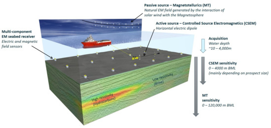
Figure 1.
CSEM acquisition scheme and the sensitivity below the mud line (BLM) of the MT and CSEM methods. Courtesy of EMGS.
The first applications of CSEM surveys in hydrocarbon exploration began in the early 2000s [4]. Currently, the method is widely applied for several applications, such as sub-basalt [5] or sub-salt [6] imaging, to help to make drilling decisions and target ratings [7,8], and reservoir appraisal [9].
Reservoir monitoring and surveillance are the new frontier for the CSEM method [10,11]. Several synthetic studies have shown the CSEM time-lapse sensitivity in order to solve for resistivity changes associated with fluid substitution [12,13,14,15,16]. However, to date, only one 4D survey has been reported in the literature [17].
Most 4D studies are limited to ranges from pre-production to periods of up to 28 years of injection and monitoring [18]. An exception is provided by the long-term study of [15], where they investigated 110 years of CO2 injection in a deep saline aquifer for storage purposes. This situation is particularly favorable for the CSEM method, as the target’s resistivity increases with time, thus yielding stronger anomalies. On the other hand, oil–water or gas–water substitutions decrease the target’s resistivity, thus producing weaker anomalies. For long-term monitoring, this effect must be taken into account.
In the Brazilian offshore margin, several mature oilfields were discovered in the late 1970s to 1980s [19,20,21]. The Albian to Miocene siliciclastic turbidite reservoirs contain medium-gravity oil (909–945 kg/m), and seawater injection was the primary method for improving oil recovery for over 30 years of oil production [21]. Due to the difference in resistivity between the oil and the injected saltwater, all of these fields can be considered candidates for future 4D CSEM surveys. However, after over 30 years of production and seawater injection, long-term time-lapse CSEM monitoring would still be feasible for these mature fields. To confirm this hypothesis, we developed an iterative workflow (Figure 2) that includes reservoir flow simulations in a realistic Earth model to produce an updated Earth model, forward modeling of the synthetic CSEM response, inverse modeling of the synthetic CSEM response, extraction of relevant EM attributes at the reservoir interval, and their correlation with petrophysical parameters.
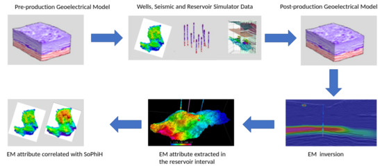
Figure 2.
Flowchart representation of the CSEM time-lapse monitoring workflow.
In the present work, we show that the anomalous transverse resistance (ATR), a key parameter in defining the CSEM response of a given reservoir, exhibits a strong linear correlation with the SoPhiH maps obtained from the fluid-flow simulations. Reservoir engineers and reservoir geologists commonly use these maps to identify/predict sweet spots in a given reservoir [22]. Consequently, by inverting the CSEM data to estimate the reservoir’s ATR, we can evaluate the sweet spots by using CSEM on a scale similar to that regularly used by reservoir specialists.
This workflow was successfully applied to the deepwater Marlim reservoir. Reservoir resistivity models were computed with a fluid simulator applied to the Marlim R3D (MR3D) model [23] for the simulated years of 2021 and 2031, thus representing time gaps of 30 or 40 years, respectively, with respect to the pre-production base year of 1991. The proposed workflow can be implemented in similar reservoir settings worldwide.
2. Geological Setting of Marlim Field
The Marlim oilfield is situated in the northeastern portion of the offshore Campos Basin, Brazil. Marlim is a mature heavy oil field discovered in 1985 at water depths ranging from 600 to 1200 m (Figure 3). The oil production started in 1991 [24].
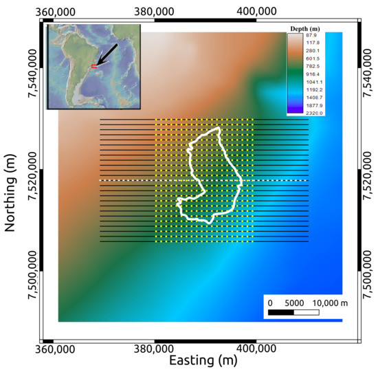
Figure 3.
Geometry of the acquisition superimposed on the bathymetric map of the MR3D area. The reservoir outline is displayed as a white line. The yellow dots are receiver locations distributed in a regular grid with 1000 m spacing. The black lines are source towlines that are evenly spaced at 1000 m. Towline 04Tx013 is highlighted with the black and white striped line. Source locations are spaced every 100 m along each towline.
The sedimentary section of the Campos Basin can be divided into three megasequences linked with three tectonic stages: rift, transitional, and drift (Figure 4).
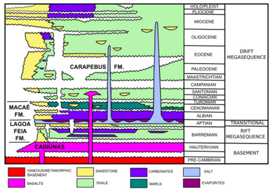
Figure 4.
Simplified stratigraphic chart of the Campos Basin, modified from [29].
The basement of the Campos Basin is composed of Cabiúnas basalts (Hauterivian). The rift sequence is characterized by the Barremian lacustrine deposits of the Lagoa Feia Formation (Barremian). These sediments are thought to be the most significant source rocks in the basin. The transitional sequence includes conglomerates, carbonates, and mainly evaporites, which were deposited in a calm tectonic phase during the Aptian. The drift stage comprises two marine sequences: the shallow-water calcarenites and calcilutites of the Macaé Formation (Albian to Cenomanian) and the deep-water turbiditic sedimentation of the Carapebus Formation (Turonian to upper Miocene). These turbiditic systems hold the most relevant petroleum reservoirs in the Campos Basin [25]. According to [26], the deposition of the Carapebus Formation was greatly influenced by salt tectonics.
The heavy oil reservoirs in Marlim Field comprise an Oligocene/Miocene deep-water turbidite system of the Carapebus Formation (Figure 4). They constitute a set of amalgamated sandstone bodies identified as Marlim sandstone [27]. The turbidite sedimentation occurred under the control of a regional northwest–southeast-trending transfer fault system [20]. This system produced the pathway for the sedimentation, reworking, and disposal of many deep-water turbiditic reservoirs in the Campos Basin [28].
The Marlim oilfield has been investigated by several authors, who focused on 3D and 4D seismic studies for reservoir characterization and monitoring [30,31,32,33]. Recently, the authors of [23,34] made available, respectively, the open-source MR3D geoelectric model and the associated CSEM dataset. MR3D is a realistic anisotropic benchmark model for the turbiditic reservoir of the Brazilian continental margin. The model combines fine-scale stratigraphy and complex oil-filled reservoirs at a depth of 2650 m (Figure 5).
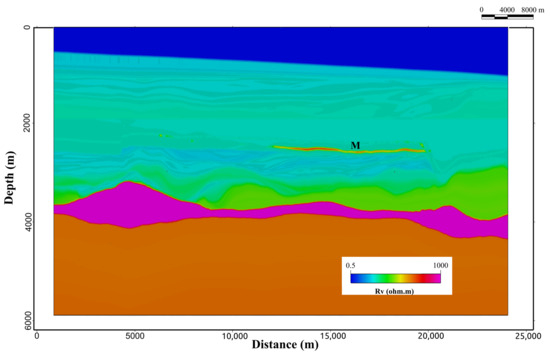
Figure 5.
Cross-section of the MR3D model’s vertical resistivity along the east–west towline, 04Tx013 (location in Figure 3). Marlim’s oil-prone turbidites (M) appear as thin resistive bodies.
The VTI model combines fine-scale stratigraphy and complex oil-filled reservoirs embedded in a geological background comprised of Oligo-Miocene shales, post-salt carbonates, a thick Aptian salt layer, and pre-salt-carbonates [34]. Table 1 presents the resistivity values of the background geology.

Table 1.
Resistivity values of the background geology according to the MR3D model.
The facies of the Marlim reservoirs are formed by clean sandstones with high porosity values in the range of 26–32% [33]. The reservoirs have a variable thickness of up to 125 m, with a mean of 80 m [24]. Figure 6 shows the isopach map between the top and bottom of the reservoir with the four main northwest–southeast-trending thick turbidite lobes (A–D in Figure 6) that compose the main production zones of Marlim Field [35]. The authors of [23] assigned the values of 70 ohm.m and 140 ohm.m to the reservoir facies for Rh and Rv, respectively. This condition assumes the 1991 pre-production scenario (base year), i.e., a fully charged reservoir.
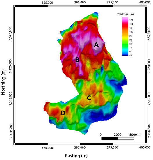
Figure 6.
Isopach map of the MR3D reservoir. A, B, C, and D, are thick turbidite lobes.
3. Time-Lapse Workflow
3.1. Marlim Time-Lapse Model
CSEM time-lapse studies can be sorted into two main groups: data-domain studies, where CSEM datasets from base and monitoring surveys are directly compared [36,37], and model-domain studies, where a comparison is made by using the recovered models for each survey [16,18]. The latter approach’s main advantage is that it avoids or minimizes the need for strict repeatability requirements when analyzing the 4D response in the data domain.
In the present work, we extend the findings of [18] in monitoring the effects of CSEM due to changes in resistivity resulting from water saturation changes within the reservoir. Other effects will not be considered, as they have been thoroughly examined by [16].
The starting point of our workflow (Figure 2) is the pre-production resistivity scenario—in our case, the MR3D model (Figure 5). There is a long-term seismic time-lapse project for Marlim [31], and new seismic acquisitions are planned for 2021 and 2031. To reproduce Marlim’s CSEM time-lapse response (recorded at the seafloor) to changes in the reservoir conditions, we use results simulated for 2021 and 2031 with a fluid-flow simulator to create a subsurface cellular model. To date, no CSEM data have been acquired in Marlim; hence, we consider 2021 as the synthetic base survey and 2031 as the monitoring survey.
The simulator yields the pressure and saturation variations for each planned seismic survey acquisition, for which we consider the marine CSEM survey acquisition. These variations are then converted into either seismic impedances or velocity and resistivity values. The reservoir connection, the relative scarcity of gas, the relative permeability curves’ advantageous properties, and the field locations lead to the seawater injection of 600,000 barrels/day as the most feasible method for pressure maintenance and oil recovery [24]. The injection design is an alternate line drive around the whole reservoir.
We used a flow simulation model based on previous geological and geophysical studies [23,33] for the Marlim reservoir with a stratigraphic grid [38] of 2,246,976 cells (332 [i] × 376 [j] × 18 [k]). The in situ water and oil saturations were populated cell by cell in the flow simulator, assuming that there was no transition zone between oil and water. A water saturation of 100% below the oil–water contact (OWC) and an oil saturation of about 80% above the OWC, up to an irreducible water saturation limit of about 20%, were considered. Two single relative permeability curves were defined for the Marlim reservoir zone (one corresponding to oil and one to water), and the post-production saturation behavior was modeled using these permeability curves and a conventional black oil simulator [39].
In the seismic method, the Gassmann equation [40] is customarily used to understand the impacts of fluids and the porous rock matrix in the data. In the CSEM method, the equivalent equation originates from Archie’s law [41], where the total formation resistivity is determined from the fluid resistivity ,
where is the brine saturation filling the pore space, n is the saturation exponent, which is regularly assumed to be 2, and F is the formation factor, which is a function of the sediment texture and is independent of :
where a is the formation tortuosity, which is generally considered to be at unity [42], is the porosity, and m is the cementation factor (frequently considered as 2 in clastic sediments).
Using the typical parameters for tortuosity and cementation and saturation exponents from [41], one may generate unrealistically high resistivity values that conflict with those computed from the well log analysis. We observed this in reservoirs with low porosity values [18]. For this reason, i.e., to have a standard workflow to apply to study any reservoir of the Brazilian offshore margin, we opted for the use of the generalized approach of [42]:
where is the resistivity of the pore fluid (). Substituting F into Equation (1), we get
The vertical and horizontal resistivity values in the reservoir—Rv and Rh, respectively—are computed by using Equation (4) with the following steps:
- 1.
- Take the harmonic averages that approximate the reservoir’s Rv and Rh resistivity values within the reservoir interval for the resistivity well logs at 36 selected wells. Estimate the water saturation (Sw) using the base year’s flow simulator (1991) and the Rv and Rh for the oil-saturated sand and water-saturated sand.
- 2.
- Estimate and n by linear regression of the logarithms of Rv, Rh, and Sw of the base year (1991) for the selected wells.
- 3.
- Apply Equation (4) for the simulated years of 2021 2031 by using the estimated and n parameters and the corresponding water saturation from the fluid simulation interpolated into the finely discretized (100 × 100 × 20 m) MR3D forward computational mesh [34].
We assume in the present work that the resistivity changes are restricted to the reservoir area, while the background remains fixed. Consequently, the reservoir resistivity values are imprinted into the background resistivity model (Table 1) to calculate the CSEM forward responses for 2021 and 2031 by employing a finite-difference time-domain (FDTD) CSEM algorithm [43]. We used the same detailed mesh discretization adopted by [34] with a total of almost 90 million cells (Table 2).
Table 2.
Mesh used in the MR3D finite-difference forward- modeling exercise.
To illustrate the effect of the water-flooding simulation on the Marlim reservoir’s resistivity, in Figure 7, we show the true ATR (anomalous transverse resistance) maps for the base year (2021) and the monitoring year (2031). The ATR, a key parameter for describing the CSEM response of a given reservoir, is the product of the target thickness and the difference between the target and background resistivity values. Herein, we define the true ATR as the ATR derived from the flow simulation experiment and described by Equation (5):
where and denote the height and the vertical resistivity of a given cell within the flow simulator’s stratigraphic grid. is the true background resistivity surrounding the MR3D reservoir (Oligo-Miocene shales in Table 1). The indices define the cell’s position in the grid, and the K index describes the layer where the cell is located in a model with N layers.
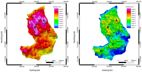
Figure 7.
True time-lapse ATR maps of the MR3D reservoir calculated from the flow simulation experiment. (Left panel) The base year, 2021. (Right panel) The monitoring year, 2031. A, B, C, and D are anomalous resistivity zones associated with the reservoir’s thickest portions (Figure 6).
The true ATR maps show four prominent NW–SE-trending anomalies (A, B, C, and D in Figure 7). These anomalies are associated with thick turbidite lobes, which are the main producing zones of the Marlim Field [35]. The true ATR maps show the expected decreases in the reservoir’s resistivity associated with the fluid substitution for several years of water injection. In 2031, after 40 years of production, the resistivity values are predicted to drop to about 50% of those of the base year (2021). Nevertheless, the resistivity pattern indicates that the turbidite lobes are still anomalous (as they are in 2021), indicating that these areas are the principal remaining sweet spots in the reservoir.
3.2. CSEM Data
Figure 3 shows an outline of the synthetic CSEM survey in the MR3D. The survey comprises 25 E–W towlines spaced by 1 km and a dense 1 × 1 km grid of 500 seabed receivers.
We used a 3D forward-modeling parallelized commercial fast finite-difference time-domain (FDTD) CSEM modeling algorithm [43] to compute all six electromagnetic field components—Ex, Ey, Ez, Hx, Hy, and Hz—for the six source frequencies of 0.125, 0.25, 0.5, 0.75, 1, and 1.25 Hz. These frequencies are within the frequency range of multi-client CSEM campaigns over the Brazilian offshore margin, including the Campos Basin [44].
The electromagnetic fields of the noise-free data were calculated with 0.1 s time steps, with a maximum number of 200,000 time steps and a convergence accuracy of . We normalized the electric fields with the dipole moment. Then, we added multiplicative noise with a 1% standard deviation according to the strategy of [45], as well as noise floors of V/Am for the electric fields and m for the magnetic fields.
We considered a horizontal electric dipole source that was towed 30 m above the seabed. The transmitter current was directed along the towing direction, and the inline and broadside data were registered with up to 11 km offsets [34].
The synthetic CSEM data were generated for the 2021 and 2031 monitoring cases described above. The modeling exercise produced high-quality data with a source–receiver offset of up to 11 km for the lower frequencies and maximum ranges of 5 to 6 km for the higher frequencies (Figure 8).
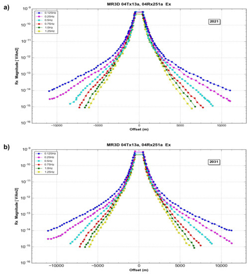
Figure 8.
Typical data for the MR3D model showing the overall good quality of the inline electric field. Site 04Rx25a. (a) Base survey (2021); (b) monitoring survey (2031).
3.3. Inversion of the Time-Lapse Response
We ran an unconstrained 3D anisotropic inversion of the synthetic CSEM data for the base year and the monitoring case. The 3D inversion was based on a quasi-Newton BFGS optimization algorithm [46], and it typically took less than 50 iterations to reach an acceptable standard RMS target misfit. A conventional L1 smoothness norm was used for the logarithm of the resistivity values.
We upscaled the forward background resistivity mesh to the inversion mesh, which was discretized as a regular grid with 200 × 200 × 50 m cells, leading to a total of almost 9 million cells (Table 3) with two free inversion parameters, Rv and Rh.
Table 3.
Mesh used in the BFG inversions of the MR3D time lapse.
An important question that is frequently raised in CSEM inversions is about the knowledge of the background resistivity. This question is more critical in exploration surveys, where, customarily, few or no wells are available for constraining the inversion. This is not an issue in the MR3D case. With over 30 years of exploration in the area, hundreds of wells have been drilled and logged, thus providing a unique knowledge of the background resistivity values (Table 1). This background—not including the resistive salt layer—was used as the starting model for the inversions. The high-resistivity contrast between the conductive sediments and the extremely high-resistivity salt (1000 ohm.m) could lock the inversion solutions in a local minimum, where it would not be possible to update the resistivity at the reservoir cells. The resistivity in the reservoir area in the starting model was set to the same layer’s background resistivity, assuming that there were no hydrocarbons. Once the inversion began to run, it built up the reservoir resistivity until the acceptable misfit was achieved.
Figure 9 shows the recovered Rv of the final model for the base year’s (2021) unconstrained anisotropic inversion co-rendered with seismic amplitude data. The cross-section along the 04Tx13 line (Figure 9a) shows a smooth Rv anomaly with a low vertical resolution around the thin turbidite reservoir of the MR3D at 2600 m depth (M in Figure 9a). On the other hand, when visualized on the 2600 m depth slice, the recovered Rv exhibits a high horizontal resolution, and the anomaly borders have an excellent match with the MR3D reservoir outline (Figure 9b).
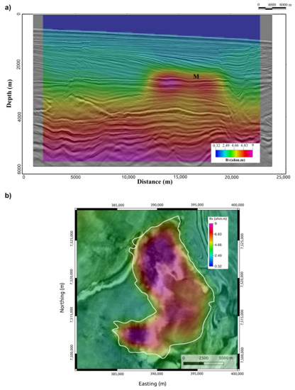
Figure 9.
Rv recovered from the 2021 3D anisotropic inversion co-rendered with the seismic amplitude of the MR3D. (a) Cross-section along the 04Tx13 line. The thin oil-prone turbidites in the MR3D (M) appear as anomalous seismic amplitude reflections [33]. (b) Recovered Rv extracted at the 2600 m depth slice. The MR3D reservoir outline is shown in the white line.
We continue with the interpretation of the inversion results by focusing on the reservoir area and extracting the recovered ATR on the top of the MR3D horizon (Figure 10) by adopting the following equation:
where denotes the reservoir thickness, which is calculated as the difference between the horizons of the top of the MR3D and the base of the MR3D; comprises the RMS of the recovered vertical resistivity attribute extracted in the [−50, +200 m] depth window around the top of the MR3D horizon. is the surrounding average background vertical resistivity recovered with the 3D anisotropic inversion.
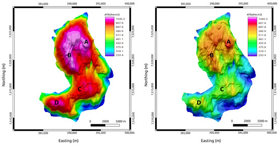
Figure 10.
Recovered ATR maps of the MR3D reservoir calculated from the 3D anisotropic inversion. (Left panel) The base year (2021). (Right panel) The monitoring year (2031). A, B, C, and D are anomalous resistivity zones associated with the reservoir’s thickest portions (Figure 6).
Comparing Figure 7 and Figure 10, we observe that the CSEM inversion-based recovered ATR explains the main features observed in the true maps. The four main anomalous producing zones within the MR3D reservoir were correctly identified. The time-lapse effect was also observed with the decrease in the ATR amplitude responses associated with the production’s fluid substitution.
3.4. SoPhiH Maps
Geologists have distinguished oil and gas prospects by mapping reservoirs’ water saturation, porosity, and thickness. Indeed, measurements of these three parameters have proved to be reliable predictors of reservoir productivity. They can be blended into a single calculation, the SoPhiH map [22], which provides knowledge on the remaining oil thickness in the studied reservoir. The SoPhiH map can be used as a subsidiary tool for defining the best drilling location for production or injection wells.
In the present paper, we calculated the true SoPhiH maps from the dynamic flow simulation model using Equation (7):
where and represent the porosity and oil saturation, respectively, of a given cell in the stratigraphic grid.
The true SoPhiH maps presented in Figure 11 show the same four prominent NW–SE-trending anomalous zones that appear in the true ATR maps (Figure 7). As discussed previously, these anomalies are correlated with thick turbidite lobes, which are the main producing zones of Marlim Field [35].
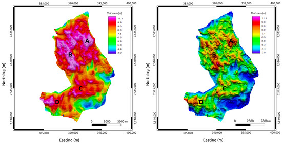
Figure 11.
True time-lapse SoPhiH maps of the MR3D reservoir calculated from the flow simulation experiment. (Left panel) The base year (2021). (Right panel) The monitoring year (2031). A, B, C, and D are anomalous oil zones associated with the reservoir’s thickest portions (Figure 6).
The decrease in the oil thickness column due to the fluid substitution for several years of water injection is also observed in the time-lapse maps of Figure 11. The true SoPhiH maps corroborate the true ATR findings, indicating the turbidite lobes as the most important remaining sweet spots in the MR3D reservoir.
3.5. ATR–SoPhiH Correlation
As discussed previously, the fluid-flow simulation experiment in the MR3D reservoir allowed the estimation of two petrophysical parameters linked with the same oil saturation and geological conditions—the ATR (Figure 7) and SoPhiH (Figure 11) maps. This presents an opportunity to investigate the existence of a relationship between these two parameters.
To that end, we applied a cross-plot analysis (Figure 12) to confirm that the ATR, a well-known attribute calculated from CSEM surveys, can be used to quantitatively predict the SoPhiH maps for the time-lapse monitoring of the MR3D reservoir. Thus, this goes beyond the traditional semi-quantitative interpretations that are ordinarily performed on CSEM data.
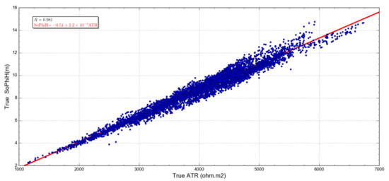
Figure 12 presents the cross-plot of the true ATR (Figure 7) and the true SoPhiH (Figure 11) attributes as determined by the flow simulation. A strong linear relationship is observed between the reservoir properties, with a correlation coefficient R greater than 98% (R = 0.981). The ATR is directly proportional to SoPhiH, i.e., an increase in the ATR attribute relates to an increase in the remaining oil column thickness. This behavior aligns with Archie’s law [41], where the rock resistivity increases with the hydrocarbon content.
4. Discussion
After establishing a linear relationship between the ATR and the SoPhiH attributes, it is now possible, by using the CSEM data inversion, to estimate the absolute values for SoPhiH within the MR3D time-lapse study.
The central idea is to cross-plot the recovered ATR from a CSEM survey (Figure 10) with the true SoPhiH computed from the flow simulation (Figure 11) to find the linear relationship between them in the 2021 and 2031 base and monitoring surveys (Figure 13), respectively. Next, we apply the discovered relationship to the ATR map to generate the converted SoPhiH map for each simulated year (Figure 14). These maps are the final product of our time-lapse workflow.
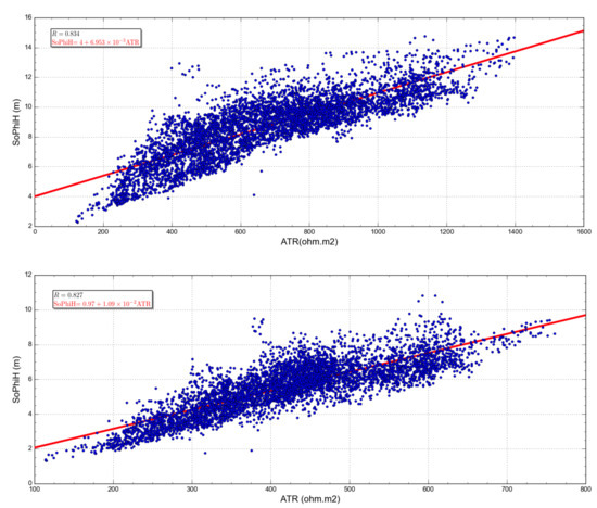
Figure 13.
Relation between the ATR recovered from the CSEM inversion (Figure 10) and the true SoPhiH (Figure 11) calculated from the flow simulation. The red line shows the best least-square fit to the data (blue circles). (Upper panel) The 2021 base year with a correlation coefficient R of 0.834. (Lower panel) The monitoring year 2031 with a correlation coefficient R of 0.827.
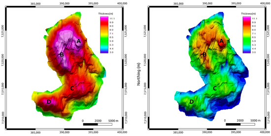
Figure 14.
SoPhiH maps predicted based on the CSEM inversion of the MR3D reservoir. (Left panel) The base year (2021). (Right panel) The monitoring year (2031). A, B, C, and D are anomalous oil zones associated with the reservoir’s thickest portions; compare with the true SoPhiH maps of the flow simulation in Figure 11.
Figure 13 exhibits the cross-plot between the recovered ATR (Figure 10) and the true SoPhiH (Figure 11) for 2021 and 2031. Due to the smoothing and spreading of the recovered Rv (Figure 9) obtained with the inversion process [46], the estimated ATR values are lower than the actual ones. Nevertheless, the linear relationship between the estimated ATR and SoPhiH maps is still observed for both years. The overall correlation coefficient R exceeds 80% in both cases, which is 0.834 and 0.827 for 2021 and 2031.
SoPhiH Prediction
Equations (8) and (9) define the relation between the CSEM-inversion-based ATR and the SoPhiH of the flow simulations for 2021 and 2031, respectively.
where SoPhiH and ATR are the predicted SoPhiH and ATR for 2021. SoPhiH and ATR are the predicted SoPhiH and ATR for 2031.
Figure 14 shows the SoPhiH maps predicted for the time-lapse monitoring of the MR3D by employing Equations (8) and (9). Note the remarkable agreement between the predicted responses and their actual values (Figure 11). The predicted responses reproduced the principal anomalous oil zones within the MR3D reservoir, with a few small discrepancies in the short-wavelength anomaly range, which can be associated with the smoothing of anomalies built into the inversion process.
More importantly, the time-lapse response in 2031 is still detectable, making CSEM surveys a viable choice for monitoring the fluid substitution in Marlim Field.
5. Conclusions
We presented a CSEM data interpretation workflow for time-lapse reservoir monitoring purposes. As part of the workflow, using a fluid-flow simulator, we demonstrated a linear relationship between the ATR attribute and the SoPhiH maps. Consequently, using that relationship, one can delimit the remaining oil sweet spots in a given reservoir.
The proposed workflow comprises fluid-flow simulations in a realistic reservoir model, forward modeling of the updated model’s synthetic CSEM response, inverse modeling of the synthetic CSEM response, and extract-based inversion of the EM attributes at the reservoir interval, as well as their association with the petrophysical parameters derived from the flow simulation.
We applied the workflow to the mature Marlim oilfield by simulating the CSEM time-lapse responses on the MR3D, a complex open-source geological model that is available for download and free usage on the Zenodo platform. The experiment was performed for 2021 and 2031, representing 30 and 40 years, respectively, of oil production with seawater injection.
The 3D forward modeling was accomplished by using a refined mesh of approximately 90 million cells. The resistivity background was kept constant, and changes due to fluid substitution were allowed only within the reservoir boundaries. The CSEM data from 2021 and 2031 were inverted by using an unconstrained 3D inversion algorithm; such inversions are regularly used in CSEM interpretations. The recovered resistivity values had a low vertical resolution but showed an excellent correlation with the outline of the MR3D reservoir. More importantly, we were also able to recover the resistivity differences associated with reservoir production and fluid substitution.
Advancing beyond the estimation of resistivity, we calculated the SoPhiH maps from the CSEM-based inversion of the ATR attribute for each simulated year by using a rock physics approach. These predicted maps strongly correlated with the ones obtained by the flow simulator.
The proposed CSEM workflow contributes to the correct identification of bypassed oil within a given reservoir, as the CSEM data are sensitive to oil-prone resistors. Therefore, it is a valuable tool for the quality control of flow simulation predictions. Our workflow is very flexible and can be applied to any similar reservoirs worldwide, as it has been proven to be an efficient method for forecasting SoPhiH maps from CSEM data inversions. It consequently represents a significant advance in time-lapse reservoir characterization.
Author Contributions
Conceptualization, P.T.L.M. and J.L.C.; methodology, P.T.L.M., J.L.C., and L.M.A.; validation, P.T.L.M., J.L.C., and L.M.A.; writing—original draft preparation, P.T.L.M.; writing—review and editing, J.L.C., L.M.A., A.R.V., and R.C.S.; supervision, A.R.V. and R.C.S.; project administration, A.R.V. and R.C.S. All authors have read and agreed to the published version of the manuscript.
Funding
This research was funded by Petrobras.
Institutional Review Board Statement
Not applicable.
Informed Consent Statement
Not applicable.
Data Availability Statement
The data associated with this research are confidential and cannot be released.
Acknowledgments
We are thankful to the management of Petrobras for their support and permission to publish this work. We thank Friedrich Roch for the permission to use the EMGS’s data acquisition figure. We are also grateful to Claudia Twarz for assistance with the 3D inversion code usage. We are grateful to two anonymous reviewers that helped us to improve our paper.
Conflicts of Interest
The authors declare no conflict of interest. The funders had no role in the design of the study.
Abbreviations
The following abbreviations are used in this manuscript:
| CSEM | Controlled-source electromagnetic |
| BML | Below mud line |
| VTI | Vertical transverse isotropy |
| RAR | Resistivity anisotropy ratio |
| Rv | Vertical resistivity |
| Rh | Horizontal resistivity |
| ATR | Anomalous transverse resistance |
| OWC | Oil–water contact |
| BFGS | Broyden–Fletcher–Goldfarb–Shanno |
| RMS | Root mean square |
References
- Constable, S.; Srnka, L.J. An introduction to marine controlled-source electromagnetic methods for hydrocarbon exploration. Geophysics 2007, 72, WA3–WA12. [Google Scholar] [CrossRef]
- Landrø, M. Discrimination between pressure and fluid saturation changes from time-lapse seismic data. Geophysics 2001, 66, 836–844. [Google Scholar] [CrossRef]
- MacGregor, L.; Tomlinson, J.; Maver, K.G. CSEM acquisition methods in a multi-physics context. First Break 2019, 37, 67–72. [Google Scholar] [CrossRef]
- Ellingsrud, S.; Eidesmo, T.; Johansen, S.; Sinha, M.C.; MacGregor, L.M.; Constable, S. Remote sensing of hydrocarbon layers by seabed logging (SBL): Results from a cruise offshore Angola. Lead. Edge 2002, 21, 972–982. [Google Scholar] [CrossRef]
- Panzner, M.; Morten, J.P.; Weibull, W.W.; Arntsen, B. Integrated seismic and electromagnetic model building applied to improve subbasalt depth imaging in the Faroe-Shetland Basin. Geophysics 2016, 81, E57–E68. [Google Scholar] [CrossRef]
- Zerilli, A.; Buonora, M.P.; Menezes, P.T.; Labruzzo, T.; Marçal, A.J.; Silva Crepaldi, J.L. Broadband marine controlled-source electromagnetic for subsalt and around salt exploration. Interpretation 2016, 4, T521–T531. [Google Scholar] [CrossRef]
- Buonora, M.P.P.; Correa, J.L.; Martins, L.S.; Menezes, P.T.L.; Pinho, E.J.C.; Silva Crepaldi, J.L.; Ribas, M.P.P.; Ferreira, S.M.; Freitas, R.C. mCSEM data interpretation for hydrocarbon exploration: A fast interpretation workflow for drilling decision. Interpretation 2014, 2, SH1–SH11. [Google Scholar] [CrossRef]
- Lyrio, J.C.S.O.; Menezes, P.T.L.; Correa, J.L.; Viana, A.R. Multiphysics anomaly map: A new data fusion workflow for geophysical interpretation. Interpretation 2020, 8, B35–B43. [Google Scholar] [CrossRef]
- Miotti, F.; Zerilli, A.; Menezes, P.T.L.; Crepaldi, J.L.; Viana, A.R. A new petrophysical joint inversion workflow: Advancing on reservoir’s characterization challenges. Interpretation 2018, 6, SG33–SG39. [Google Scholar] [CrossRef]
- Sambo, C.; Iferobi, C.C.; Babasafari, A.A.; Rezaei, S.; Akanni, O.A. The role of 4d time lapse seismic technology as reservoir monitoring and surveillance tool: A comprehensive review. J. Nat. Gas Sci. Eng. 2020, 80, 103312. [Google Scholar] [CrossRef]
- Black, N.; Zhdanov, M.S. Active geophysical monitoring of hydrocarbon reservoirs using electromagnetic methods. In Active Geophysical Monitoring; Elsevier: Amsterdam, The Netherlands, 2020; pp. 69–95. [Google Scholar]
- Black, N.; Wilson, G.A.; Gribenko, A.V.; Zhdanov, M.S.; Morris, E. 3D inversion of time-lapse CSEM data based on dynamic reservoir simulations of the Harding field, North Sea. In SEG Technical Program Expanded Abstracts 2011; Society of Exploration Geophysicists: Tulsa, OK, USA, 2011; pp. 666–670. [Google Scholar]
- Katterbauer, K.; Hoteit, I.; Sun, S. EMSE: Synergizing EM and seismic data attributes for enhanced forecasts of reservoirs. J. Pet. Sci. Eng. 2014, 122, 396–410. [Google Scholar] [CrossRef]
- Salako, O.; MacBeth, C.; MacGregor, L. Potential applications of time-lapse CSEM to reservoir monitoring. First Break 2015, 33, 35–46. [Google Scholar] [CrossRef]
- Ayani, M.; Grana, D.; Liu, M. Stochastic inversion method of time-lapse controlled source electromagnetic data for CO2 plume monitoring. Int. J. Greenh. Gas Control 2020, 100, 103098. [Google Scholar] [CrossRef]
- Shantsev, D.V.; Nerland, E.A.; Gelius, L.J. Time-lapse CSEM: How important is survey repeatability? Geophys. J. Int. 2020, 223, 2133–2147. [Google Scholar] [CrossRef]
- Ziolkowski, A.; Parr, R.; Wright, D.; Nockles, V.; Limond, C.; Morris, E.; Linfoot, J. Multi-transient electromagnetic repeatability experiment over the North Sea Harding field. Geophys. Prospect. 2010, 58, 1159–1176. [Google Scholar] [CrossRef]
- Zerilli, A.; Labruzzo, T.; Golfre’Andreasi, F.; Menezes, P.D.T.L.; Crepaldi, J.L.S.; Alvim, L.D.M. Realizing 4D CSEM Value on Deep Water Reservoirs—The Jubarte Case Study. In Proceedings of the 80th EAGE Conference and Exhibition 2018, Copenhagen, Denmark, 11–14 June 2018; European Association of Geoscientists & Engineers: Houten, The Netherlands, 2018; Volume 2018, pp. 1–5. [Google Scholar]
- Lucchesi, C.F.; Gontijo, J.E. Deep Water Reservoir Management: The Brazilian Experience. In Proceedings of the Offshore Technology Conference, Houston, TX, USA, 4–7 May 1998. [Google Scholar] [CrossRef]
- Lourenço, J.; Menezes, P.T.L.; Barbosa, V.C.F. Connecting onshore-offshore Campos Basin structures: Interpretation of high-resolution airborne magnetic data. Interpretation 2014, 2, SJ35–SJ45. [Google Scholar] [CrossRef]
- Dumas, G.E.S.; Freire, E.B.; Johann, P.R.S.; Silva, L.S.; Vieira, R.A.B.; Bruhn, C.H.L.; Pinto, A.C.C. Reservoir Management of the Campos Basin Brown Fields. In Proceedings of the Offshore Technology Conference, Houston, TX, USA, 30 April–3 May 2018. [Google Scholar] [CrossRef]
- Brinkerhoff, R. Pitfalls in Geological Mapping Within Unconventional Plays. In Proceedings of the AAPG Annual Convention and Exhibition, Calgary, AB, Canada, 21 June 2016. [Google Scholar]
- Carvalho, B.R.; Menezes, P.T.L. Marlim R3D: A realistic model for CSEM simulations-phase I: Model building. Braz. J. Geol. 2017, 47, 633–644. [Google Scholar] [CrossRef]
- Shecaira, F.S.; Daher, J.S.; Gomes, A.C.A.; Capeleiro Pinto, A.C.; Filoco, P.R.; Gomes, J.A.T.; Freitas, L.C.S.; Balthar, S. Injeção de Água no Campo de Marlim—Uma Abordagem Integrada para o Gerenciamento de Reservatórios. In Proceedings of the Rio Oil & Gas Expo and Conference, Rio de Janeiro, Brazil, October 2000; Brazilian Petroleum Institute—IBP: Rio de Janeiro, Brazil, 2000; pp. 1–9. [Google Scholar]
- Bruhn, C.T.; Gomes, J.; Lucchese, C., Jr.; Johann, P. Campos Basin: Reservoir Characterization and Management-Historical Overview and Future Challenges. In Proceedings of the Offshore Technology Conference, Houston, TX, USA, 5–8 May 2003. [Google Scholar]
- Mohriak, W.U.; Macedo, J.M.; Castellani, R.T. Salt tectonics and structural styles in the deep-water province of the Cabo Frio region, Rio de Janeiro, Brazil. In Salt Tectonics: A Global Perspective: AAPG Memoir 65; Jackson, M.P.A., Roberts, D.G., Snelson, S., Eds.; AAPG: Tulsa, OK, USA, 1996; Chapter 13; pp. 273–304. [Google Scholar]
- Peres, W.E. Shelf-fed turbidite system model and its application to the Oligocene deposits of the Campos Basin, Brazil. AAPG Bull. 1993, 77, 81–101. [Google Scholar]
- Cobbold, P.R.; Meisling, K.E.; Mount, V.S. Reactivation of an obliquely rifted margin, Campos and Santos basins, southeastern Brazil. AAPG Bull. 2001, 85, 1925–1944. [Google Scholar] [CrossRef]
- Guardado, L.R.; Spadini, A.R.; Brandão, J.S.L.; Mello, M.R. Petroleum System of the Campos Basin, Brazil. In Petroleum Systems of South Atlantic Margins: AAPG Memoir 73; Mello, M.R., Katz, B.J., Eds.; AAPG: Tulsa, OK, USA, 2000; Chapter 22; pp. 317–324. [Google Scholar]
- Sansonowski, R.C.; de Oliveira, R.M.; Júnior, N.M.d.S.R.; Bampi, D.; Junior, L.F.C. 4D seismic interpretation in the Marlim Field, Campos Basin, offshore Brazil. In Proceedings of the 10th International Congress of the Brazilian Geophysical Society, Rio de Janeiro, Brazil, 19–23 November 2007; European Association of Geoscientists & Engineers: Houten, The Netherlands, 2007; pp. 1–6. [Google Scholar]
- Johann, P.; Sansonowski, R.; Oliveira, R.; Bampi, D. 4D seismic in a heavy-oil, turbidite reservoir offshore Brazil. Lead. Edge 2009, 28, 718–729. [Google Scholar] [CrossRef]
- Fainstein, R.; Jamieson, G.; Hannan, A.; Biles, N.; Krueger, A.; Shelander, D. Offshore Brazil Santos Basin exploration potential from recently acquired seismic data. In Proceedings of the 7th International Congress of the Brazilian Geophysical Society, Salvador, Brazil, 28–31 October 2001; European Association of Geoscientists & Engineers: Houten, The Netherlands, 2001; pp. 1–6. [Google Scholar]
- Nascimento, T.M.; Menezes, P.T.; Braga, I.L. High-resolution acoustic impedance inversion to characterize turbidites at Marlim Field, Campos Basin, Brazil. Interpretation 2014, 2, T143–T153. [Google Scholar] [CrossRef]
- Correa, J.L.; Menezes, P.T. Marlim R3D: A realistic model for controlled-source electromagnetic simulations—Phase 2: The controlled-source electromagnetic data set. Geophysics 2019, 84, E293–E299. [Google Scholar] [CrossRef]
- Mutti, E.; Cunha, R.S.; Bulhoes, E.; Arienti, L.M.; Viana, A.R. Contourites and turbidites of the Brazilian marginal basins. In Proceedings of the AAPG Annual Convention & Exhibition, Houston, TX, USA, 6–9 April 2014. [Google Scholar]
- Orange, A.; Key, K.; Constable, S. The feasibility of reservoir monitoring using time-lapse marine CSEM. Geophysics 2009, 74, F21–F29. [Google Scholar] [CrossRef]
- Andréis, D.; MacGregor, L. Using CSEM to monitor production from a complex 3D gas reservoir—A synthetic case study. Lead. Edge 2011, 30, 1070–1079. [Google Scholar] [CrossRef]
- Caumon, G.; Mallet, J.L. 3D Stratigraphic models: Representation and stochastic modelling. In Proceedings of the IAMG 2006, International Association for Mathematical Geology XIth International Congress, Liege, Belgium, 3–8 September 2006. [Google Scholar]
- Fanchi, J.R. Chapter 11—Traditional Model Study. In Principles of Applied Reservoir Simulation, 4th ed.; Fanchi, J.R., Ed.; Gulf Professional Publishing: New York, NY, USA, 2018; pp. 195–219. [Google Scholar] [CrossRef]
- Gassmann, F. Elastic waves through a packing of spheres. Geophysics 1951, 16, 673–685. [Google Scholar] [CrossRef]
- Archie, G.E. The electrical resistivity log as an aid in determining some reservoir characteristics. Trans. AIME 1942, 146, 54–62. [Google Scholar] [CrossRef]
- Glover, P.W.J. A generalized Archie’s law for n phases. Geophysics 2010, 75, E247–E265. [Google Scholar] [CrossRef]
- Maaø, F.A. Fast finite-difference time-domain modeling for marine-subsurface electromagnetic problems. Geophysics 2007, 72, A19–A23. [Google Scholar] [CrossRef]
- Lorenz, L.; Pedersen, H.T.; Buonora, M.P. First results from a Brazilian mCSEM calibration campaign. In Proceedings of the 13th International Congress of the Brazilian Geophysical Society & EXPOGEF, Rio de Janeiro, Brazil, 26–29 August 2013; Society of Exploration Geophysicists and Brazilian Geophysical Society: Rio de Janeiro, Brazil, 2013; pp. 131–136. [Google Scholar]
- Mittet, R.; Morten, J.P. Detection and imaging sensitivity of the marine CSEM method. Geophysics 2012, 77, E411–E425. [Google Scholar] [CrossRef]
- Zach, J.; Bjørke, A.; Støren, T.; Maaø, F. 3D inversion of marine CSEM data using a fast finite-difference time-domain forward code and approximate Hessian-based optimization. In SEG Technical Program Expanded Abstracts 2008; Society of Exploration Geophysicists: Tulsa, OK, USA, 2008; pp. 614–618. [Google Scholar]


Publisher’s Note: MDPI stays neutral with regard to jurisdictional claims in published maps and institutional affiliations. |
© 2021 by the authors. Licensee MDPI, Basel, Switzerland. This article is an open access article distributed under the terms and conditions of the Creative Commons Attribution (CC BY) license (https://creativecommons.org/licenses/by/4.0/).