Abstract
Nowadays, fuel cells are becoming a real alternative to power several applications, from portable electronic devices to cars, buses, or stationary facilities. Usually, a basic analysis of a fuel cell includes polarization curve test, as this method is excellent to characterize the behavior of a fuel cell as a whole, because it integrates all the different physical process that happens inside in current and voltage signals. On the other hand, it does not provide accurate information of these physical processes as individual. In this research, we relate the results of polarization curve test and EIS (Electrochemical Impedance Spectroscopy) test through two mathematical expressions. Then, using equivalent electrical circuit elements to model EIS curves, and applying the developed expressions, we correlate the EIS and polarization curve results, allowing us to interpret the physical meaning of these circuit elements and obtain a deeper vision of the internal processes that happen.
1. Introduction
There exists a general acceptance that climate change represents one of the most serious challenges humanity currently has to face. And according to [1,2,3] there is a consensus between the scientific community that climate change driven by global warming is caused by anthropogenic activities.
To diminish the effects of these activities, and taking into consideration that transport represents 24% of global CO2 emissions from energy [4], and the use of renewable energy sources implies also the deployment of energy storage solutions capable to address variable generation profile, the use of clean energy carries, where the hydrogen technologies are included, should play a central role in the global decarbonization too.
The FLHYSAFE project [5], which provided the experimental results that we use in this research, is a research project supported by the Fuel Cells and Hydrogen 2 Joint Undertaking under the European Horizon 2020 framework program for Research and Innovation (GA No 779576). Its principal goal is to show that a fuel cell based modular system can substitute a current Ram Air Turbine of a commercial aircraft, improving safety, capabilities, and reducing costs. Additionally, demonstrating that fuel cell technology fulfills all mass, volume, and maintenance requirements to be installed into a current aircraft design.
Then, in order to ease the use of fuel cell technologies in transport means, the creation of procedures that allow us to know the state of health of the fuel cells and characterize their performance are becoming mandatory. Currently there are several studies, which propose different diagnostic tools to study ageing processes and failure causes in fuel cells [6,7,8,9]. However, the necessary equipment to implement these procedures could be easily embarked in transport means to obtain in-situ measurements, this should not be complex and expensive and the number of sensors should not be enormous, but the opposite, they have to be easy to install and robust. Thus, we deduce that they should basically consist of current, voltage, temperature, humidity, and flow-meter sensors, to obtain the energy production of the stack and temperature, humidity, and mass-flow to characterize the intake gases.
Additionally, if we analyze the fuel cell characterization tests that could fit with the previous premises of using the defined list of sensors, they do not need big and/or complex equipment in the way that it can be installed in a vehicle, and they only cause negligible effects during measurements. We decided to reduce the list to polarization curve test and Electrochemical Impedance Spectroscopy (EIS) test.
Polarization curve test [10,11,12] would probably be the most basic fuel cell characterization test. This test can be thought of as a non-continuous succession of equilibrium states, where the fuel cell goes from one state to another varying the working current value. In other words, it is a semi-stationary test. This test is very useful to synthesize the general performance of a fuel cell, so it treats the cell as a whole, integrating all the effects and physical phenomena in a response of voltage and current, from there we can obtain the general health state of the stack, but from this data it is not easy to deduce what kind of events are happening inside the stack.
The Electrochemical Impedance Spectroscopy test [13,14,15,16] basically consists of applying an electrical stimulus (a known tiny periodic voltage or current signal) to electrodes at different frequencies and obtaining a response (a resulting current or voltage). This response can be transformed into an equivalent electric circuit, in other words, into a combination of serial-parallel collection of resistances, capacitors, Warburg diffusion elements… where any of these electric components tries to represent any physical process that happens inside the stack, so this technique allows to obtain a deeper insight of what is happening in stack than the polarization curve test. EIS is considered to play an important role in electrochemistry and materials science, and it is expected that this role will be enhanced in coming years.
Commonly, the polarization curve test is used to study the effects that the operating conditions and their variations have on the fuel cell performance and in the degradation processes [17,18,19,20] and EIS test are applied to study the evolution of the fuel cell internal resistance in function of operating conditions, detect hydrogen crossover flow, and assess the hydric conditions of fuel cells [21,22,23,24,25,26,27]. However, another possibility would be to study the state of health of a fuel cell combining V-I curve and EIS results tests, and through a parametric analysis of a model obtain extra information about the physical processes that can cause fuel cell degradation [28,29].
In this article, we present two mathematical expressions that can establish a link between these two techniques, and we describe how to use them to obtain the internal information of a fuel cell. Preliminary results of the first equation were presented at the European Hydrogen Energy Conference 2018 [30], but in this article, we present a new and more robust mathematical expression that solves some issues of the first equation, this is simpler but does not present a physical solution at I = 0 A. Previously, we applied the Polarization Curve and EIS techniques on the short fuel cell stack of FLHYSAFE project to obtain experimental results that we used to validate the mathematical models.
2. Equipment and Methods Description
This section is divided in two points. In the first one, we describe the used equipment and test methodology to carry out the tests and the main characteristics of the tested fuel cell, and in the second point, we derive the two mathematical expressions that allow us to link the results of the polarization curve and EIS tests.
2.1. Equipment and Test Methodology Descriptions
In this work, we tested the nearest single cell to inlet gases of a short stack, which is composed of six LT PEM cells with an active area of 170 cm2 each cell, and platinum based catalytic layer.
To obtain the experimental results, we performed a polarization curve test, carrying out an EIS test at every current step, once the voltage values will be steady. The experiments were conducted at constant stoichiometry of 1.5 in anode and 2.0 in cathode and relative humidity of 50%, the working pressure and temperature 1.3 bara and 65 °C respectively.
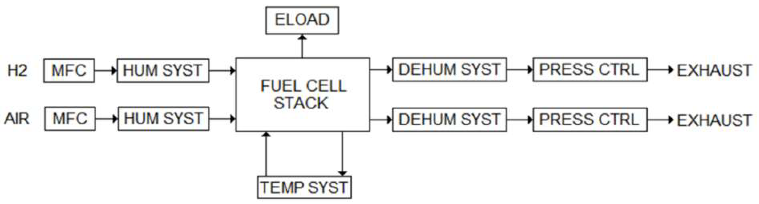
To carry out the polarization curve test, we used a fuel cell test bench that basically consists of the subsystems described in Figure 1.
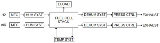
Figure 1.
Fuel cell test bench subsystems.
Furthermore, the fuel cell test bench control system allows the implementation of the polarization curve test and enables a fully automated and unattended operation fulfilling all safety requirements and reproducible test results under the specified test input parameters. Additionally, the fuel test bench included a Data Acquisition System (DAQ) with a fast enough logging rate to capture the behavior of the fuel cell at transients.
The EIS tests were carried out using a Solartron SI1287 (Electrochemical Interface) and a Solartron SI1255 HF (Frequency Response Analyzer) and to control this equipment we utilized the Zplot software. To analyze the EIS results we used the Zview software. Zplot and Zview are commercial computer programs that were developed by Scribner to perform EIS tests.
2.2. Development of Mathematical Expressions
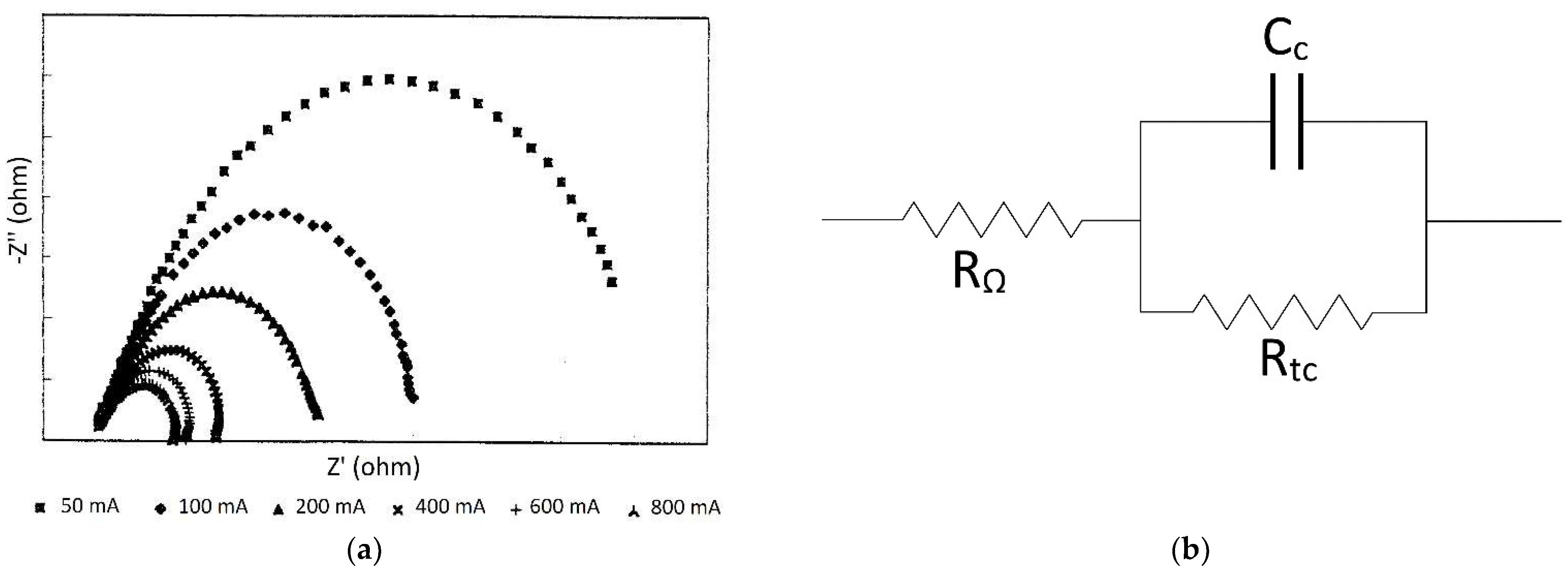
To obtain the former equation that relates the polarization curve and the Electrochemical Impedance Spectroscopy results, we start from a typical group of EIS curves, left part of Figure 2, and use the equivalent circuit at right part of Figure 2 to reproduce the fuel cell performance described by EIS curves.
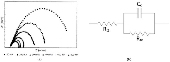
Figure 2.
(a) Typical group of EIS curves. (b) Equivalent circuit.
Where: RΩ is the ohmic resistance, Rtc is charge transfer resistance, and C is the capacitance. Figure 3 plots a generic curve of Rtc in function of current.
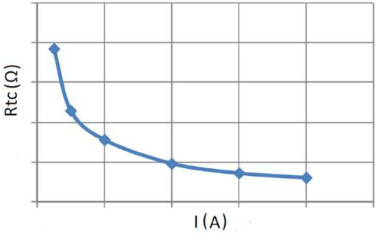
Figure 3.
Generic curve of charge transfer resistance (Rtc) vs. Current.
Studying Figure 3, we realize that the curve can be represented by a monotonic-decreasing current function. Then, supposing that the value of is given by a rational function of current, we propose Equation (1) to fit the curve prototype of Figure 3.
where: is the current; is a fitting parameter; and is a non-dimensional fitting parameter (0 ≤ b ≤ 1).
Taking into consideration that the resistance of an electric conductor is described by Equation (2).
where: is the electrical resistivity constant; is the resistance length; and is the resistance cross-section. Now, supposing the current is directly proportional to fuel cell active surface area, we define it by Equation (3).
where: is the total active surface area; and are both the resistance cross-section and is the max current of the fuel cell. Additionally, supposing that can be expressed by Equation (2), and substituting Equation (3) in Equation (2) and clearing the variable, we obtain an expression for the resistance length (, Equation (4).
Analyzing Equation (4), we realize the length of resistance increases with current, and if we consider this length could be related to the thickness of the cathode double layer, this implies the thickness of the cathode double layer should grow with the increase of current.
Furthermore, knowing that Equation (5) provides the charge of a parallel plate capacitor.
where: is the vacuum permittivity; is the relative permittivity; is the surface areas of capacitor plates; and is the separation of capacitor plates. Taking into consideration that the resistor (Rtc) and the capacitor (C) are in parallel, we make the hypothesis that and , and and are related by Equation (6).
Therefore, combining Equations (4)–(6), we obtain an expression that describes the capacitance behavior with current, Equation (7). This expression implies the capacitance is zero when .
Additionally, we know that Equation (8) gives the charge of a capacitor.
where: is the charge; is the voltage; and is the capacitance. Now, supposing that the charge of a capacitor should be proportional to its plate area, we can write Equation (9).
where: K is a constant of proportionality. Then, combining Equations (7)–(9), we obtain the Equation (10).
This voltage should correspond to the voltage drop caused by cathode activation overpotential. In other words, the energy of activation overpotential is used to charge the capacitor and this voltage loss grows with current.
Additionally, if we perform a dimensional analysis on Equation (10), we obtain that the expression is dimensionally correct. As the units of parameters and variables are: ; ; ; ; ; ; ; ; and .
Finally, supposing that corresponds to cathode activation overpotential, we propose the Equation (11) as candidate to describe a fuel cell polarization curve.
where: is the voltage of fuel cell; is the Open Circuit Voltage; and .
Using the Equation (11) to fit polarization curve test results, we get good results, but if we analyze the Equation (1), we realize that is not defined at I = 0 A, then to solve this issue we propose to use Equation (12) to fit the curve prototype of Figure 3 instead of Equation (1).
where: is a fitting parameter. Then, using Equation (12) and operating as we did to obtain the First Mathematical Expression, we get the Equation (13).
Furthermore, if in this case we define as the addition of two magnitudes in order to avoid tends to infinite, as when .
where: is the separation of capacitor plates when ; and the other magnitudes are defined as usual. Then, combining Equations (5), (6), and (14), we obtain a new expression to capacitance.
Now, solving the equation system (6), (8), and (15), we get a new expression to capacitor voltage.
If we analyze Equation (16), we can see is an unknown variable, to obtain an expression for we substitute in Equation (15) and clear . After that, replacing by this expression in Equation (15) and taking into consideration that , we obtain a new equation for where all variables and parameters are defined.
where: is the maximum charge of the capacitor, is the capacitance at , and the other magnitudes are defined as usual. Furthermore, if we compare Equations (10) and (17), we can identify the first addend of the Equation (17) with Equation (10), or in other words, the first addend would correspond to the cathode activation overpotential, while the second addend is the values of when . Then, taking into consideration this, and operating as we did to derive Equation (11), we obtain a new equation to model a fuel cell polarization curve, and in this case, the new equation is defined in the whole range of currents.
where: is the Nernst equation voltage. Additionally, if we group terms, we will obtain Equation (19), which is equal to Equation (11) except for the parameter .
3. Results
At this point, we apply polarization curve and EIS tests on a single cell of the Short-Stack of FLHYSAFE project. This cell was located at the extreme of the Short-Stack next to the entrance of gases. Using the presented methodology we explain in detail how to relate the results of both tests and extract internal information from the tested cell.
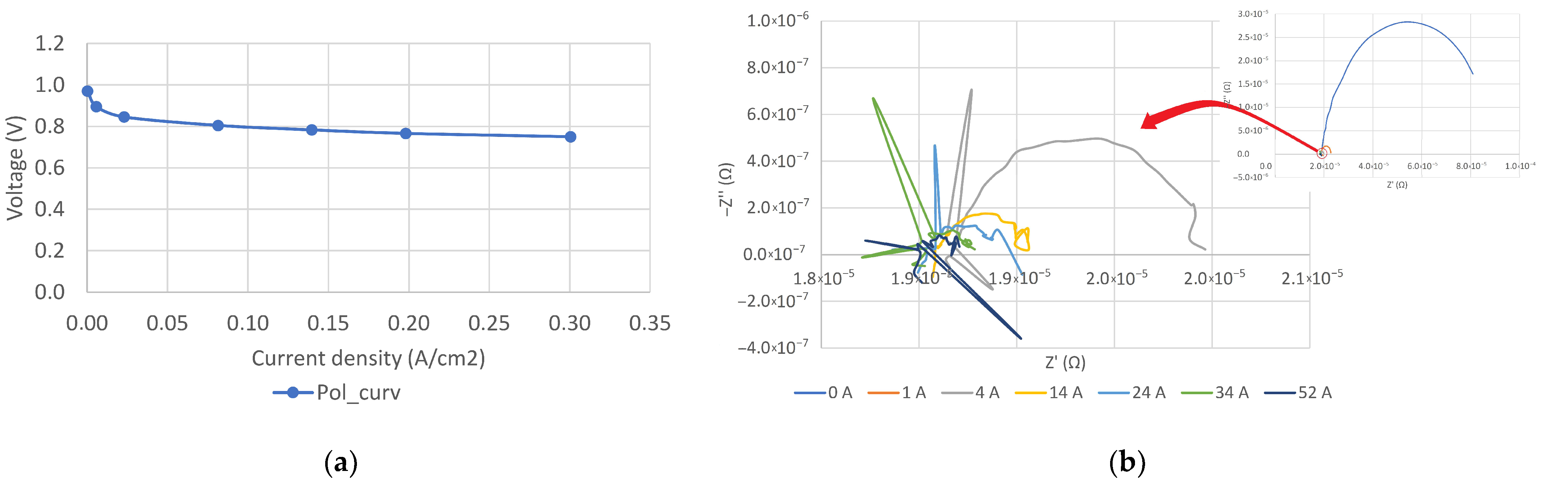
Firstly, we performed a polarization curve test and for each current step we carried out an EIS test, once the standard deviation of the last 10 voltage measurement was less than 1%, this is the criteria that we used to establish the fuel cell behavior was steady and stable. The results of these tests appear in Figure 4.
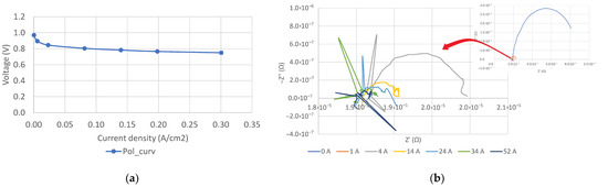
Figure 4.
Experimental results: (a) polarization curve; (b) EIS curves.
As can be seen, all EIS curves are represented in in (b) Figure 4, but as the EIS curve at Open Circuit Value (OCV) is much bigger in comparison to the rest, we zoom the EIS curves from I = 4 A to I = 52 A. Now, using the Zwiev software we fit each one of the EIS curves with the Equation (20) in order to extract the ohmic resistance (RΩ), and the charge transfer resistance (Rtc), these values are collected in Table 1. The Equation (20) is the mathematical transposition of the equivalent circuit of Figure 2b.
where: and is the frequency of EIS stimulus.

Table 1.
Ohmic resistance (RΩ), charge transfer resistance (Rtc), capacitance (C) fitting values of raw EIS curves. Equation (20).
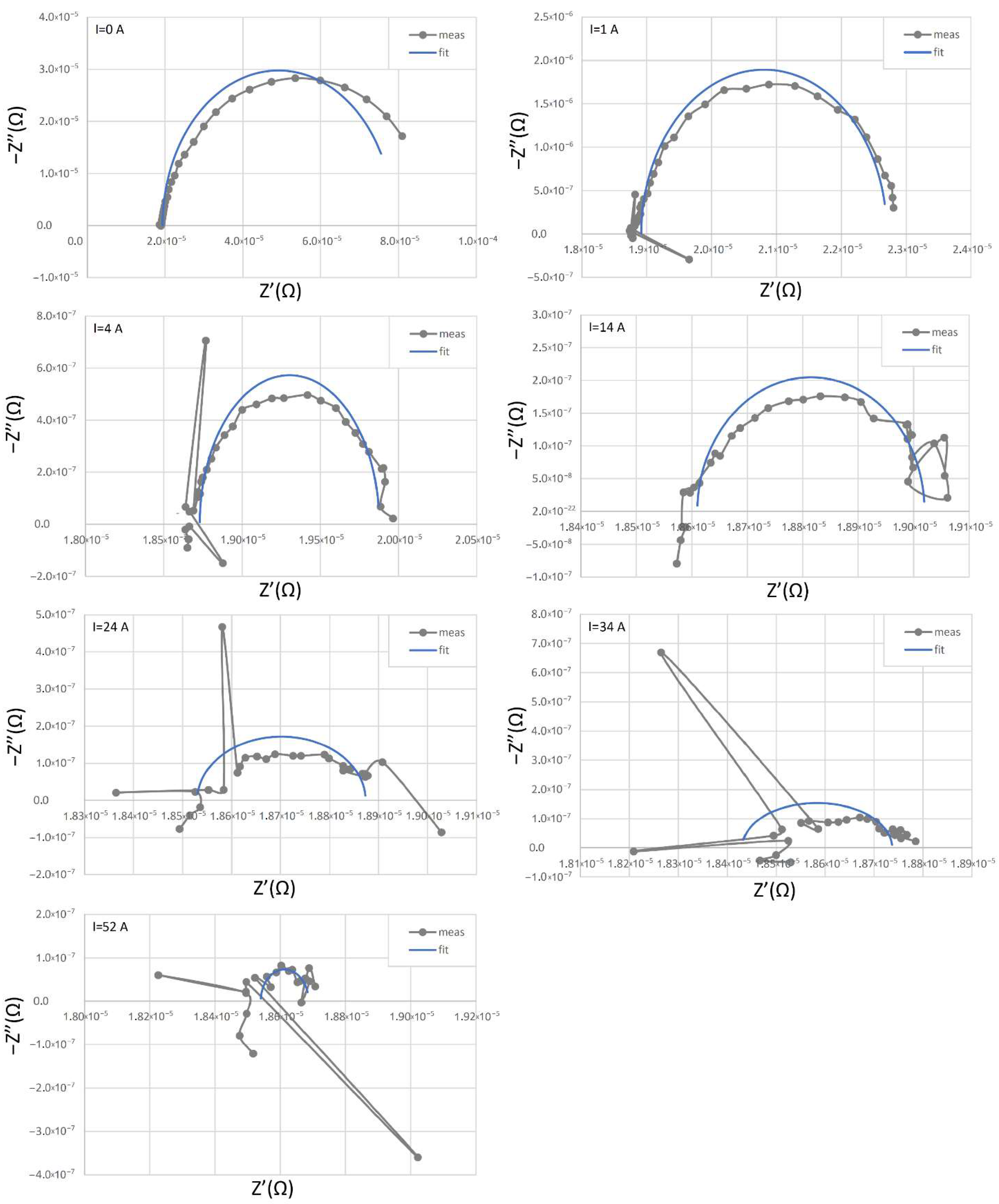
Now, individually representing the raw EIS curve value along with its fitting curve for each current, we get Figure 5. If we analyze Figure 5, we realize the existence of anomalous points. To discriminate these points, we calculate the distance between the measured and the fitted values for each point through Equation (21).
where: is the measured impedance real part of i-point; is the measured impedance imaginary part of i-point; is the fitted impedance real part of i-point; is the fitted impedance imaginary part of i-point; is the maximum value of the all measured impedances real parts; is the minimum value of the all real measured impedances parts; is the maximum value of the all measured impedances imaginary parts; and is the minimum value of the all measured impedances imaginary parts.
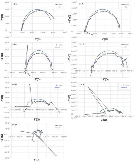
Figure 5.
Raw EIS curve along with its fitting curve for each current. Equation (20).
Now, defining outlier as the point which distance doubles the mean distance, Equation (22):
where: N is the total number points of a EIS curve.
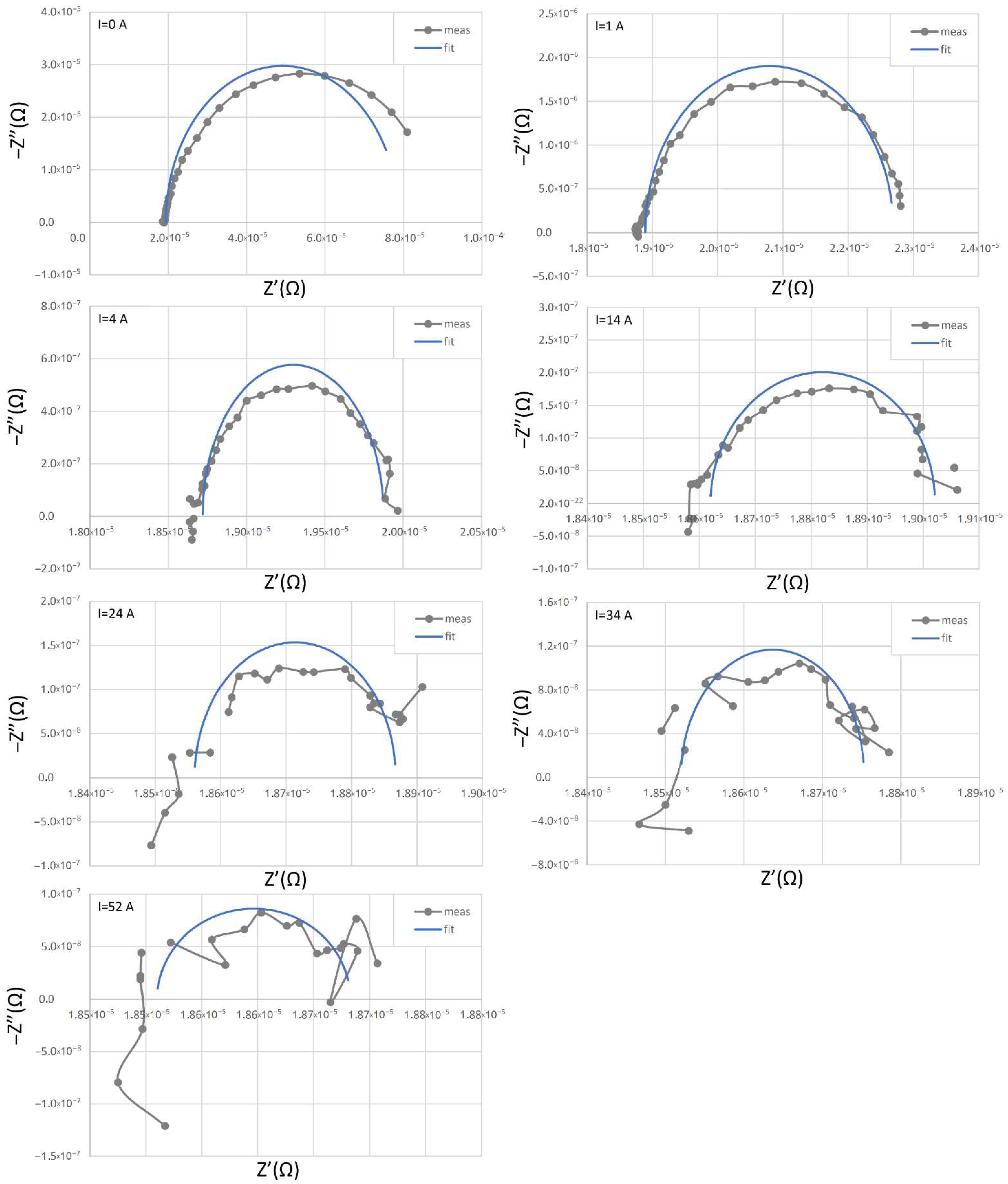
Then removing the outliers of EIS curves, and using the Equation (20) to fit the filtered EIS curves, we obtain new values for the ohmic resistance (RΩ), and the charge transfer resistance (Rtc). Now, we represent the filtered EIS curves along with their fit curves in Figure 6.
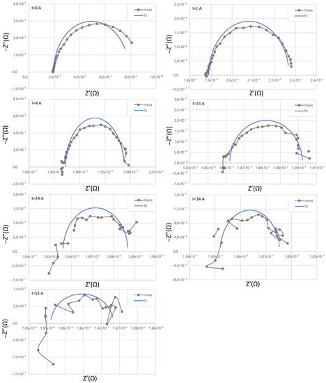
Figure 6.
Filtered EIS curve along with its fitting curve for each current. Equation (20).
Additionally, the ohmic resistance (RΩ), and the charge transfer resistance (Rtc) values obtained from fitting the filtered EIS curves are given in Table 2.
Table 2.
Ohmic resistance (RΩ), charge transfer resistance (Rtc), and capacitance (C) fitting values of filter EIS curves. Equation (21).
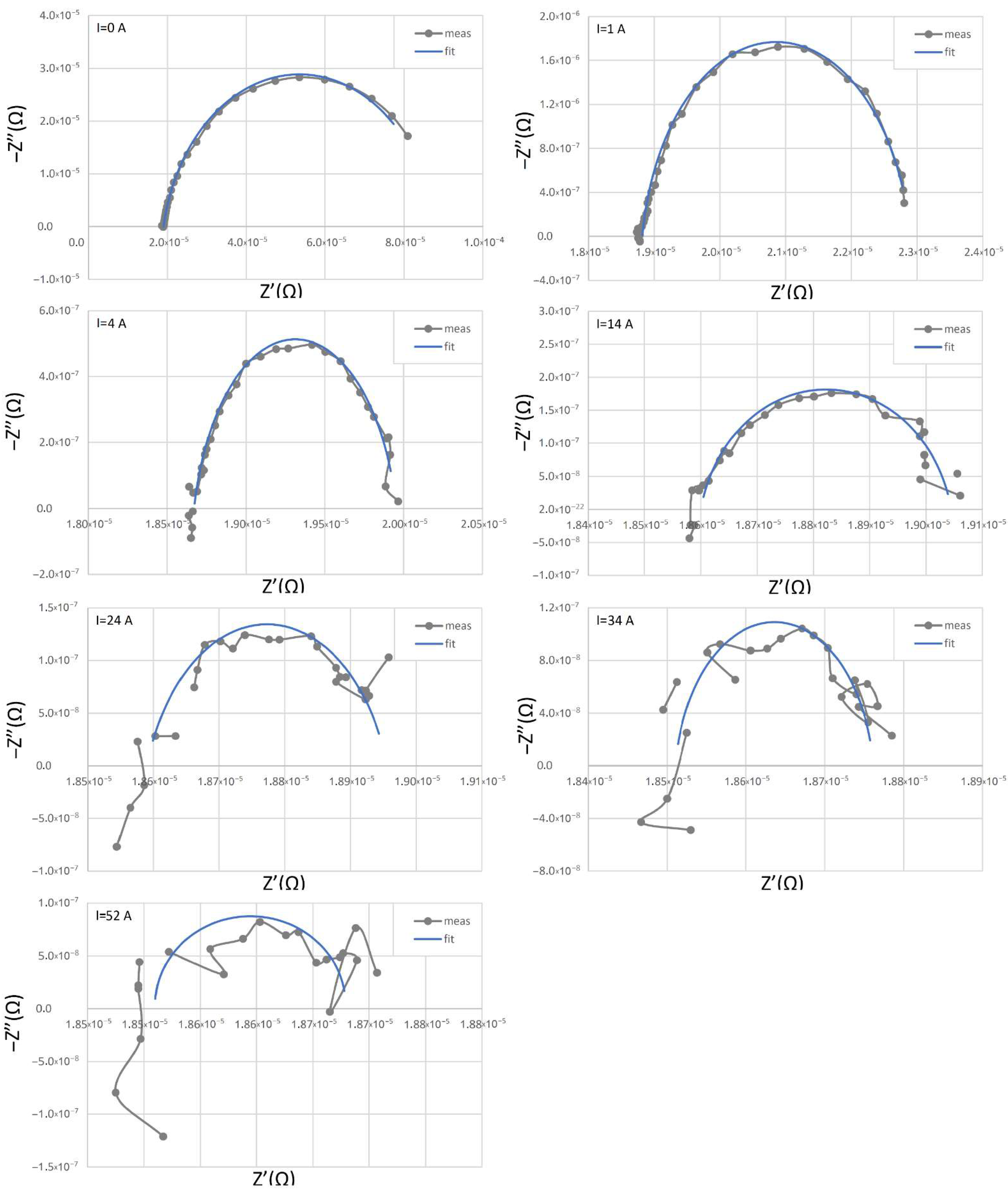
Comparing Figure 5 and Figure 6, we can appreciate that outlier filtering has improved the fitting, especially in the curves for high currents. If we analyze which were the anomalous points, we find the majority of them have a frequency of 100 or 200 Hz, so it is reasonable to suppose they can be a network harmonic (50 Hz), and therefore they really are a sporous measurement. On the other hand, the filtering criteria found nine outliers for the EIS curve at I = 0 A, but we considered this was caused because the selected equivalent circuit of Figure 2b does not properly fit this case. In order to improve the fitting accuracy, we decided to change the capacitor of equivalent circuit of Figure 2b by a constant phase element (CPE). The CPE frequently substitutes capacitors to simulate inhomogeneities of a system as rough and porous surfaces. The Equation (23) describes the behavior of the equivalent circuit of Figure 2b when the capacitor is replaced by a CPE. The impedance of a CPE is described by the expression , where: is the capacitance of CPE (F); and is the non-dimensional exponent of the CPE phase. If p = 1 then gives the impedance of a capacitor.
Then using the Equation (23) to adjust the filter EIS curves, we obtain the fitting values of Ohmic resistance (RΩ), charge transfer resistance (Rtc), and capacitance (T) and phase exponent (p), given in Table 3.
Table 3.
Ohmic resistance (RΩ), charge transfer resistance (Rtc), and capacitance (T) and phase exponent (p) fitting values of filter EIS curves. Equation (23).
Now, we plot the filtered EIS curves along with the fit curves, which were obtained using Equation (23), in Figure 7. If we compare Figure 6 and Figure 7, it is clear that Equation (23) improves the fitting accuracy.
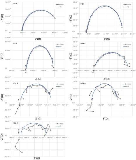
Figure 7.
Filtered EIS curve along with its fitting curve for each current. Equation (23).
Once we have obtained Rtc (Ω) for different currents Table 2 and Table 3, we are in disposition to fit the charge transfer resistance using the Equation (1).
Equivalent circuit with capacitor:
Equivalent circuit with CPE:
is the mean relative error, defined by Equation (26).
where are measured values, and are fitting values. To calculate the mean relative error for Equations (25) and (26) the value of at 0 A was not taken in consideration, as Equation (1) is not defined for this current.
Now, substituting the values of the charge transfer resistance fitted parameters in Equation (11) and adjusting this expression to polarization curve of Figure 4a, we obtain the following fitted Equations (27) and (28).
Equivalent circuit with capacitor:
Equivalent circuit with CPE:
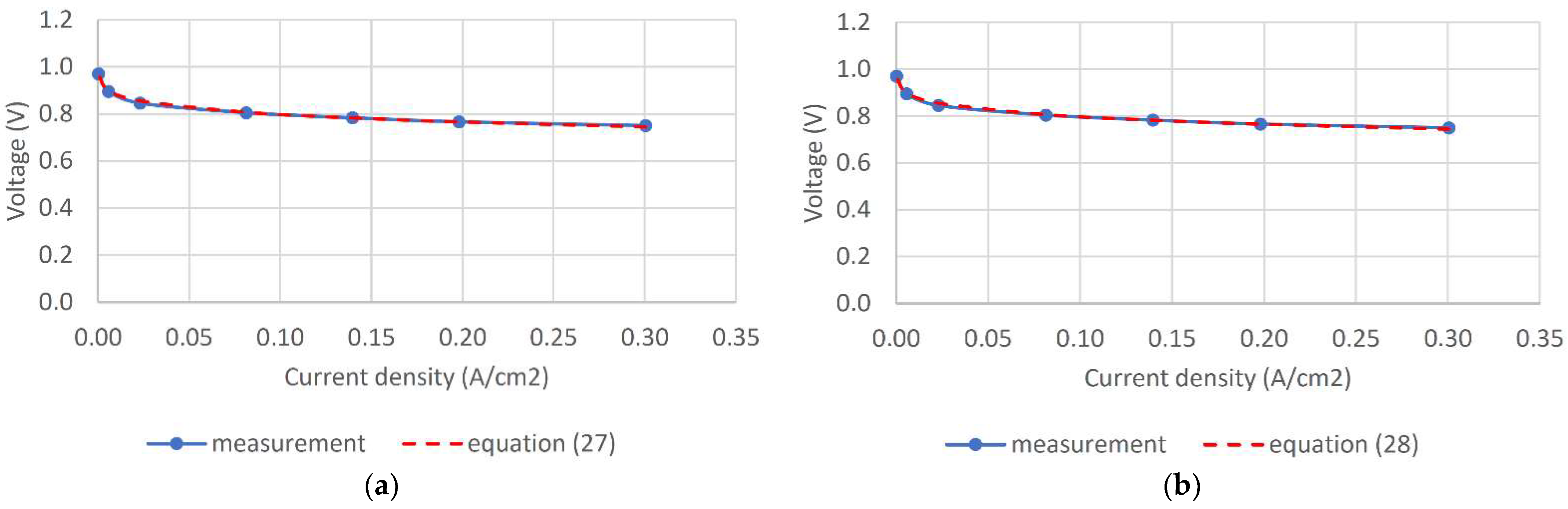
To better appreciate the fitting accuracy, we represent together the polarization curve of Figure 4a and the fitting curves of Equations (27) and (28) in Figure 8.
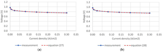
Figure 8.
Measured polarization curve and its fitting curves: (a) fitting curve of Equation (27), (b) fitting curve of Equation (28).
If we analyze Figure 8, we can see the fitting curves match well with the experimental results. Furthermore, we can observe that the ohmic resistance values of Equations (27) and (28) agree with the Rtc (Ω) values of Table 2 and Table 3, and the OCV results have physical meaning. In other words, the fitting values of Rtc (Ω) and OCV are apparently more than fitting parameters and they have physical sense.
On the other hand, if we use Equation (11) without any restrictions to fit the polarization curve of Figure 4a, we can obtain a solution, but in this case the fitting parameters do not have physical meaning, Equation (29).
Now, repeating the previous process, but using Equation (12) to fit the charge transfer resistance of Table 2 and Table 3, we obtain the following expressions.
Equivalent circuit with capacitor:
Equivalent circuit with CPE:
Then, using the parameterization, and fitting the polarization curve of Figure 4a with Equation (18), we get two expressions for fuel cell voltage.
Equivalent circuit with capacitor:
Equivalent circuit with CPE:
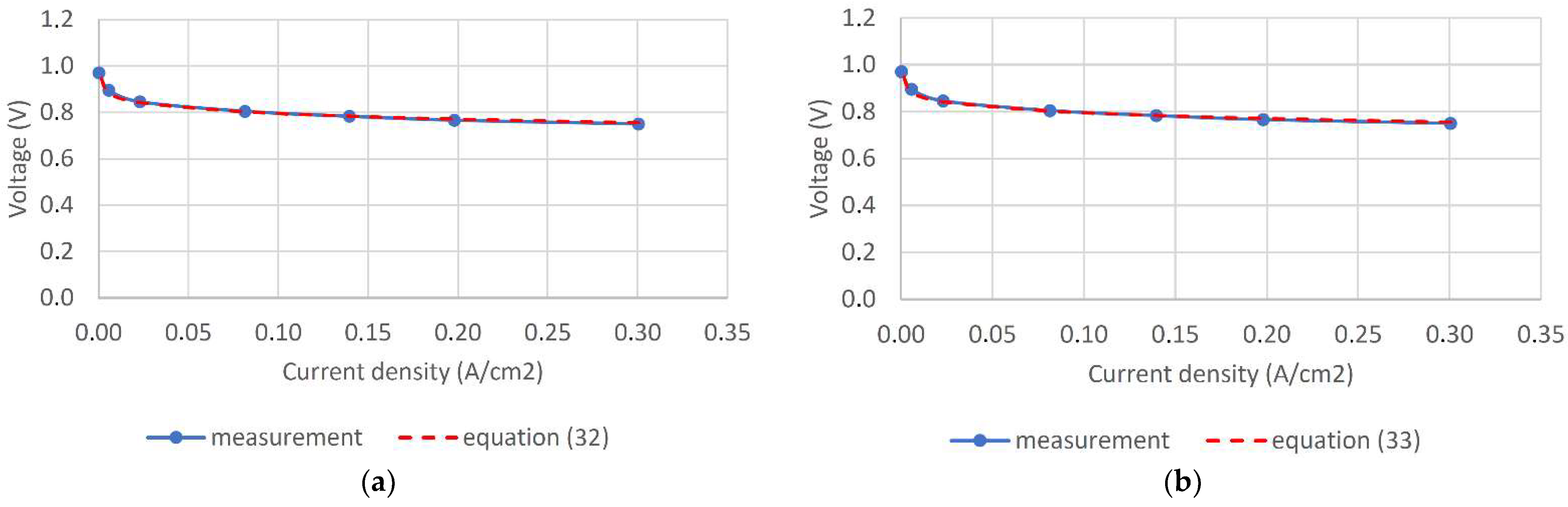
Carrying on as before, we plot together the polarization curve of Figure 4a and the fitting curves of Equations (32) and (33) in Figure 9.
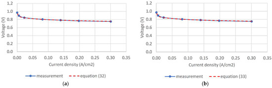
Figure 9.
Measured polarization curve and its fitting curves: (a) fitting curve of Equation (31); (b) fitting curve of Equation (32).
Now, assessing the fitting accuracy of Equations (11) and (18) to adjust a polarization curve of a fuel cell, we can see that both of them match well, and none of them does significantly better than the other. However, Equation (18) is defined in all ranges of current and provides extra information.
Then, the results of the equivalent circuit with CPE are selected arbitrarily, as repetition of the analysis process with the results of the equivalent circuit with capacitor does not provide any extra information. We can see that Equation (18) predicts the existence of a kind of current value when the load demand is zero. The parameter can be written as , then clearing we obtain, .037 A. The experimental equipment measured 0.05 A when there was no power demand.
4. Discussion
In this article, we present a new methodology that allows us to relate the results of polarization curve tests with the EIS tests. Each test provides different information of the same reality, so it is expected that the correct combination of them could provide a more complete vision of the physical phenomena that occurs inside the fuel cell.
This methodology is based on Equation (11) or Equation (18), the second one is an evolution of the first. Once they have been partially parametrized using the EIS results, they fit well with the experimental results of polarization curve tests, and the fitting parameters have physical meaning. Conversely, when the selected equation does not have restrictions, we can obtain a good fitting curve too, but in this case, the fitting parameter has no physical meaning. Therefore the hypothesis that we established to derive the equations could be correct, and they can capture the physical processes that happen inside the fuel cell. If this is right, we have developed a model that pretends to describe the dynamic of the double layer, establishing a link between the elements of Figure 4b. In other words, the variations of the resistance affects the capacitance and vice versa.
According to this model, Equation (6) describes the coupling laws between capacitor and resistor, if Equation (11) is selected to describe the fuel cell voltage dependence with current. If not, the relation between the length of resistance and the distance of capacitor parallel plates is defined by Equation (14). In any case, these coupling laws say that the variations of lengths are equal and the variations of surface areas are the opposite .
Now, taking into consideration Equation (4), the lengths are related to the thickness of the double layer, the model says this grows with current.
Concerning surface areas, we know that Equations (1) and (12) are rational functions and both indicate the resistance decreases with current but increases—this implies that active surface area or in other words the resistance surface area grows fast enough to compensate the increase. This could point out that total charge transfer resistance is the sum of parallel resistances of the ionic current paths that go through the double layer, and the number grows with the increase of current. This is expressed by Equations (34) and (35):
where: is the total charge transfer resistance, and is the resistance of i-th ionic current path. Now, considering that without loss of generality, we obtain a rational function for total charge transfer resistance that decreases with current:
Additionally, the model expresses that the double layer surface should be equal to and is constant, so if increases with current, this means that decreases. Then, taking into consideration this, and that grows with current, we obtain that capacitance should decrease with current, as it usually does according to the experimental results of Table 2 and Table 3, but not always. The discrepancy between results and this conclusion must be studied in detail, to determine its causes.
On the other hand, it is necessary to note the novelty of the research, and that it was not supported by a large number of results. Nowadays, this methodology has been applied in nine cases, obtaining positive results in all cases. We continue checking the methodology and improving the models.
5. Conclusions
In this section, we pretend to summarize the most important findings. Basically, in this research, we have obtained two prototypes of Equations (11) and (18), that can describe the behavior of an experimental polarization curve with a mean relative error inferior to 1%, and when the parameter is obtained from using one of the previously described methodologies, the values of other fitting parameters have physical meaning, allowing us to write:
where is the Open Circuit Voltage, is the Nernst Voltage and C0 is the capacitance at I = 0 A. Equation (36) implies the loss of voltage at I = 0 A is mainly caused by the formation of the double layer in cathode interface region and provides an easy way to quantify the charge of the double layer when the load is zero.
Additionally, Equation (18) provides an expression for the cathode overpotential too, Equation (37).
Equation (37) shows the cathode overpotential presents dependence with the permittivity and the resistivity of the cathode interface, and this expression can be used to obtain how the variation of the permittivity and the resistivity affects the cathode overpotential, and maybe this could be used to improve fuel cell technology.
Author Contributions
Conceptualization, G.G.; methodology, G.G.; validation, G.G.; formal analysis, G.G.; investigation, G.G. and A.C.; resources, J.M.; data curation, G.G.; writing—original draft preparation, G.G.; writing—review and editing, G.G., P.A., A.C. and J.M.; visualization, G.G.; supervision, J.M. and P.A.; project administration, P.A.; funding acquisition, P.A. and J.M. All authors have read and agreed to the published version of the manuscript.
Funding
This research received no external funding.
Institutional Review Board Statement
Not applicable. This study does not involve humans or animals.
Informed Consent Statement
Not applicable. This study does not involve humans.
Acknowledgments
This research was developed at INTA using the experimental results of FLHYSAFE Project. Funded by the Fuel Cells and Hydrogen 2 Joint Undertaking under the European Horizon2020 Framework Programme for Research and Innovation (GANo779576).
Conflicts of Interest
The authors declare no conflict of interest.
Abbreviations
| EU | European Union |
| FLHYSAFE | Fuel celL HYdrogen System for AircraFt Emergency |
| EIS | Electrochemical Impedance Spectroscopy |
| MFC | Mass Flow Controller |
| HUM SYST | Humidification System |
| DEHUM SYST | Dehumidification System |
| PRESS CTRL | Pressure Control System |
| TEMP SYST | Working Temperature Control System |
| ELOAD | Electric Load |
| DAQ | Data Acquisition System |
| Rtc | Charge transfer resistance (Ω) |
| Current (A) | |
| Fitting parameter () | |
| Fitting parameter (0 ≤ b ≤ 1). | |
| Electrical resistivity () | |
| Resistance cross-section (m2) | |
| Resistance length (m) | |
| Total active surface area (m2) | |
| Maximum current of fuel cell (A) | |
| Vacuum permittivity (Fm−1) | |
| Relative permittivity | |
| Surface area of capacitor plates (m2) | |
| Separation of capacitor plates (m) | |
| Q | Charge of capacitor (C) |
| C | Capacitance (F) |
| Voltage of capacitor (V) | |
| K | Constant of proportionality (Asm−2) |
| Fuel cell voltage (V) | |
| Open Circuit Voltage (V) | |
| Fitting parameter (Ab) | |
| Separation of capacitor plates at I = 0 A (m) | |
| Capacitance at I = 0 A (F) | |
| Nernst equation voltage (V) | |
| Cathode overpotential (V) |
References
- Powell, J. Scientists Reach 100% Consensus on Anthropogenic Global Warming. Bull. Sci. Technol. Soc. 2017, 37, 183–184. [Google Scholar] [CrossRef]
- Cook, J.; Nuccitelli, D.; Green, S.A.; Richardson, M.; Winkler, B.; Painting, R.; Way, R.; Jacobs, P.; Skuce, A. Quantifying the consensus on anthropogenic global warming in the scientific literature. Environ. Res. Lett. 2013, 8, 024024. [Google Scholar] [CrossRef] [Green Version]
- Anderegg, W.R.L.; Prall, J.W.; Harold, J.; Schneider, S.H. Expert credibility in climate change. Proc. Natl. Acad. Sci. USA 2010, 107, 12107–12109. [Google Scholar] [CrossRef] [Green Version]
- Cars, Planes, Trains: Where do CO2 Emissions from Transport Come from? Available online: https://ourworldindata.org/co2-emissions-from-transport (accessed on 1 August 2021).
- Fuel celL HYdrogen System for AircraFt Emergency Operation. Available online: https://www.flhysafe.eu/ (accessed on 1 August 2021).
- de Moor, G.; Bas, C.; Chavin, N.; Moukheiber, E.; Niepceron, F.; Breilly, N.; André, J.; Rossinot, E.; Claude, E.; Albérola, N.D.; et al. Understanding Membrane Failure in PEMFC: Comparison of Diagnostic Tools at Different Observation Scales. Fuel Cells 2012, 12, 356–364. [Google Scholar] [CrossRef]
- Zheng, Z.; Petrone, R.; Péra, M.C.; Hissel, D.; Becherif, M.; Pianese, C.; Steiner, N.Y.; Sorrentino, M. A review on non-model based diagnosis methodologies for PEM fuel cell stacks and systems. Int. J. Hydrogen Energy 2013, 38, 8914–8926. [Google Scholar] [CrossRef]
- Lin, R.H.; Xi, X.N.; Wang, P.N.; Wu, B.D.; Tian, S.M. Review on hydrogen fuel cell condition monitoring and prediction methods. Int. J. Hydrogen Energy 2019, 44, 5488–5498. [Google Scholar] [CrossRef]
- Priya, K.; Sathishkumar, K.; Rajasekar, N. A comprehensive review on parameter estimation techniques for Proton Exchange Membrane fuel cell modeling. Renew. Sust. Energ. Rev. 2018, 93, 121–144. [Google Scholar] [CrossRef]
- Malkov, T.; Pilenga, A.; Tsotridis, G.; de Marco, G. EU Harmonised Polarization Curve Test Method for Low Temperature Water Electrolysis. European Commission, Joint Research Centre, Directorate C: Energy, Transport and Climate. © European Union 2018. Available online: https://publications.jrc.ec.europa.eu/repository/bitstream/JRC104045/kjna29182enn_online.pdf (accessed on 1 August 2021).
- Mitzel, J.; Kabza, A.; Hunger, J.; Malkow, T.; Piela, P.; Laforet, H. Test Module P-08: Polarization Curve. Development of PEM Fuel Cell Stack Reference Test Procedures for Industry. STACK-TEST Project no. 303445. Fuel Cells and Hydrogen Joint Undertaking (FCH). 2015. Available online: http://stacktest.zsw-bw.de/fileadmin/stacktest/docs/Information_Material/Performance/TMs/TM_P-08_Polarisation_Curve.pdf (accessed on 1 August 2021).
- Mohsin, M.; Raza, R.; Mohsin-ul-Mulk, M.; Yousaf, A.; Hacker, V. Electrochemical characterization of polymer electrolyte membrane fuel cells and polarization curve analysis. Int. J. Hydrogen Energy 2020, 45, 24093–24107. [Google Scholar] [CrossRef]
- Yuan, X.-Z.; Song, C.; Wang, H.; Zhang, J. Electrochemical Impedance Spectroscopy in PEM Fuel Cells Fundamentals and Applications; Springer: London, UK, 2010. [Google Scholar] [CrossRef]
- Piela, P.; Malkow, T.; de Marco, G. Test Module P-10c: H2-PEMFC and DMFC Stack Electrochemical Impedance Spectroscopy. Development of PEM Fuel Cell Stack Reference Test Procedures for Industry. STACK-TEST Project no. 303445. Fuel Cells and Hydrogen Joint Undertaking (FCH). 2015. Available online: http://stacktest.zsw-bw.de/fileadmin/stacktest/docs/Information_Material/Performance/TMs/TM_P-10c_Electrochemical_Method_Impedance_Spectroscopy.pdf (accessed on 1 August 2021).
- Macdonald, J.R.; Johnson, W.B. CHAPTER 1. Fundamentals of Impedance Spectroscopy. In Theory, Experiment, and Aplications, 3rd ed.; Barsoukov, E., Macdonald, J.R., Eds.; John Wiley & Sons, Inc.: Hoboken, NJ, USA, 2018; pp. 1–20. ISBN 9781119333173. [Google Scholar]
- Lasia, A. Electrochemical Impedance Spectroscopy and Its Applications; Springer Science & Business Media: New York, NY, USA, 2014. [Google Scholar] [CrossRef]
- Hu, Z.; Xu, L.; Li, J.; Gan, Q.; Xu, X.; Song, Z.; Shao, Y.; Ouyang, M. A novel diagnostic methodology for fuel cell stack health: Performance, consistency and uniformity. Energy Convers. Manag. 2019, 185, 611–621. [Google Scholar] [CrossRef]
- Xia, L.; Zhang, C.; Hu, M.; Jiang, S.; Chin, C.S.; Gao, Z.; Liao, Q. Investigation of parameter effects on the performance of high-temperature PEM fuel cell. Int. J. Hydrogen Energy 2018, 43, 23441–23449. [Google Scholar] [CrossRef]
- Pessot, A.; Turpin, C.; Jaafar, A.; Soyez, E.; Rallières, O.; Gager, G.; d’Arbigny, J. Contribution to the modelling of low temperature PEM fuel cell in aeronautical conditions by design of experiments. Math. Comput. Simul. 2019, 158, 179–198. [Google Scholar] [CrossRef]
- Labach, I.; Rallières, O.; Turpin, C. Steady-state Semi-empirical Model of a Single Proton Exchange Membrane Fuel Cell (PEMFC) at Varying Operating Conditions. Fuel Cells 2017, 17, 166–177. [Google Scholar] [CrossRef]
- Yan, X.; Hou, M.; Sun, L.; Liang, D.; Shen, Q.; Xu, H.; Ming, P.; Yi, B. AC impedance characteristics of a 2 kW PEM fuel cell stack under different operating conditions and load changes. Int. J. Hydrogen Energy 2007, 38, 8914–8926. [Google Scholar]
- le Canut, J.M.; Abouatallah, R.M.; Harrington, D.A. Detection of Membrane Drying, Fuel Cell Flooding, and Anode Catalyst Poisoning on PEMFC Stacks by Electrochemical Impedance Spectroscopy. J. Electrochem. Soc. 2006, 153, A857–A864. [Google Scholar] [CrossRef]
- Mérida, W.; Harrington, D.A.; le Canut, J.M.; McLean, G. Characterization of proton exchange membrane fuel cell (PEMFC) failures via electrochemical impedance spectroscopy. J. Power Sources 2006, 161, 264–274. [Google Scholar] [CrossRef]
- Mousa, G.; Golnaraghi, F.; DeVaal, J.; Young, A. Detecting proton exchange membrane fuel cell hydrogen leak using electrochemical impedance spectroscopy method. J. Power Sources 2014, 246, 110–116. [Google Scholar] [CrossRef]
- Manzo, S.C.; Castillo, U.C.; Greenwood, P. Impedance Study on Estimating Electrochemical Mechanisms in a Polymer Electrolyte Fuel Cell During Gradual Water Accumulation. Fuel Cells 2019, 19, 71–83. [Google Scholar] [CrossRef]
- Tang, Z.; Huang, Q.A.; Wang, Y.J.; Zhang, F.; Li, W.; Li, A.; Zhang, L.; Zhang, J. Recent progress in the use of electrochemical impedance spectroscopy for the measurement, monitoring, diagnosis and optimization of proton exchange membrane fuel cell performance. J. Power Sources 2020, 468, 228361. [Google Scholar] [CrossRef]
- Génevé, T.; Régnier, J.; Turpin, C. Fuel cell flooding diagnosis based on time-constant spectrum analysis. Int. J. Hydrogen Energy 2016, 38, 516–523. [Google Scholar] [CrossRef]
- El Aabid, S.; Regnier, J.; Turpin, C.; Rallières, O.; Soyez, E.; Chdourne, N.; Arbigny, J.D.; Hordé, T.; Foch, E. A global approach for consistent identification of static and dynamic phenomena in a PEM Fuel Cell. Math. Comput. Simul. 2019, 158, 432–452. [Google Scholar] [CrossRef]
- Aabid, S.E.; Turpin, C.; Regnier, J.; D’Arbigny, J.; Horde, T.; Pessot, A. Monitoring of Ageing Campaigns of PEM Fuel Cell Stacks Using a Model-Based Method. Int. J. Renew. Energy Res. 2021, 11, 92–100. [Google Scholar]
- Gómez, G.; Maellas, J.; García, C.; López, E. Proposal of an equation to measure the degradation of a PEM fuel cell, using EIS results. In Proceedings of the European Hydrogen Energy Conference 2018 (EHEC 2018), Malaga, Spain, 14–16 March 2018. [Google Scholar]

Publisher’s Note: MDPI stays neutral with regard to jurisdictional claims in published maps and institutional affiliations. |
© 2021 by the authors. Licensee MDPI, Basel, Switzerland. This article is an open access article distributed under the terms and conditions of the Creative Commons Attribution (CC BY) license (https://creativecommons.org/licenses/by/4.0/).