Abstract
Due to the constant trend of building wind turbine sets and photovoltaic cells, the so-called renewable energy sources, it is important to develop a mathematical model that will allow us to analyse the economic viability of their operation. By using this model, multivariate calculations should be carried out and developed in the form of universal nomograms that will allow us to estimate this viability almost on an immediate basis. In this paper, such a model for the unit cost of electricity production from renewable energy sources is presented. It is based on a continuous-time Net Present Value notation. The multi-variant calculations performed with it take into account different subsidy levels and operating time of the renewable energy sources. The paper presents values of unit costs of electricity production from renewable energy sources and values of maximum subsidies for this production. It turns out that subsidies are necessary for renewable energy sources to exist on the energy market. An additional disadvantage is the fact that renewable energy sources are not able to provide a stable electricity supply throughout the year.
1. Introduction
In recent years, according to the European Union (EU) policy, a growing emphasis is placed on sustainability and CO reduction. Thus, alternative energy sources are being sought to meet the ever-growing demand. Meanwhile, this policy makes electricity prices higher due to rising fees for emission rights. Emerging forecasts of energy prices indicate a steady tendency in this regard [1]. Therefore, a number of countries see the opportunity in renewable energy sources to achieve ambitious low emission targets to stabilize the energy market [2,3,4,5]. The advantage of this solution is inexhaustible resources; however, the drawback is the specific conditions of energy production, such as limited operation time during the year, e.g., due to weather or geographical location. These limitations have an impact on the cost of investment, return on capital, and durability of energy supply [6,7]. In addition, specific regulations of countries and the EU itself, including the policy of subsidies, the market for CO emission rights, and the new strategy Fit for 55, play quite a significant role [8,9]. Extra research efforts are underway to show how to shape the level of subsidies and additional incentives for investors to meet demand for electricity, while at the same time to limit the unit cost of energy production to the consumer [10,11,12].
In order to select an appropriate investment strategy, an appropriate technical and economic analysis should be carried out on the basis of a mathematical model and the adopted methodology. The studies in this area can be divided into two directions. The first one uses discrete notation by means of geometric series to evaluate economic efficiency, since the discount calculus is essentially a geometric progression. Currently, in many works we can see the predominance of this direction of research [13,14,15,16,17,18,19]. However, these models require complicated and sometimes tedious calculations or sophisticated optimization algorithms, making certain assumptions which simplify the model and thus give only approximate or uncertain results. The second direction of research used in this paper is devoid of such difficulties. It is based on the time-continuous notation of economic measures such as Net Present Value (NPV), Internal Rate of Return (IRR), and Discounted Pay Back Period (DPBP), and the methodology for building, with their help, continuous mathematical models to enable techno-economic analysis of any business projects [20,21,22]. These measures cover the entire planned period of operation of the project, i.e., years of construction and operation, during which economic effects are expected to be achieved. Using them ensures taking an effective and accurate investment decision.
The advantage of a techno-economic analysis of the electric power system made with a continuous model is, among other things, the possibility of specifying which energy technologies should be invested in. It allows for predicting how the energy market is affected by the prices of energy components and unit pollution tariffs and how their values change over time. In addition, this analysis makes it possible to estimate how the value of the market is affected by the annual operating time of electricity generation sources, subsidies, the price of CO emission allowances, and capital expenditures for modernization.
Statistical analysis of RES power plant cost-effectiveness results, finding probability distribution, cumulative distribution function, variance, mean value, mode, median, confidence intervals and levels, consistency tests, etc., require the collection of huge amounts of data for RES power plants. What is more, these data have to be gathered for RES sources operating in various atmospheric conditions, since depending on these conditions, individual statistics and their variability measures will differ significantly, e.g., operating times, investment outlays (at sea they are significantly, even more than three times, higher than onshore outlays for turbine sets of the same power), and thus, the economical effectiveness of RES operation will differ substantially. Therefore, the paper presents a mathematical model in a continuous form, which is extremely important since it takes into account all possible RES operating conditions and capital expenditures. The continuous model allows inserting time-varying values for all input quantities. Thus, it allows using differential calculus to study the course of variation of the RES efficiency function, and thus, it enables to show the nature of its course, which is impossible in the case of the discrete NPV model known and used so far. It gives only a numerical value, which obviously does not make it possible to assess the nature of the course of NPV changes. So far, such a model has not been formulated by researchers around the world. Thus, the model is completely innovative, allowing to determine the economical efficiency of RES for absolutely arbitrary and time-varying parameters and input quantities affecting their operation, as well as for any time of their operation, any investment outlays, etc. Therefore, it should be once again explicitly verbis stated that the model presented in this paper makes it possible to show the nature of the time course of the economical effectiveness values of RES sources and, extremely importantly, that it is a dynamic model.
2. The Methodology in the ‘Continuous’ Record of the Analysis of the Economic Viability of Renewable Energy Sources (RES) Operation, Taking into Account the Temporal Variability of Electricity Generated by Using Them and Their Downtimes
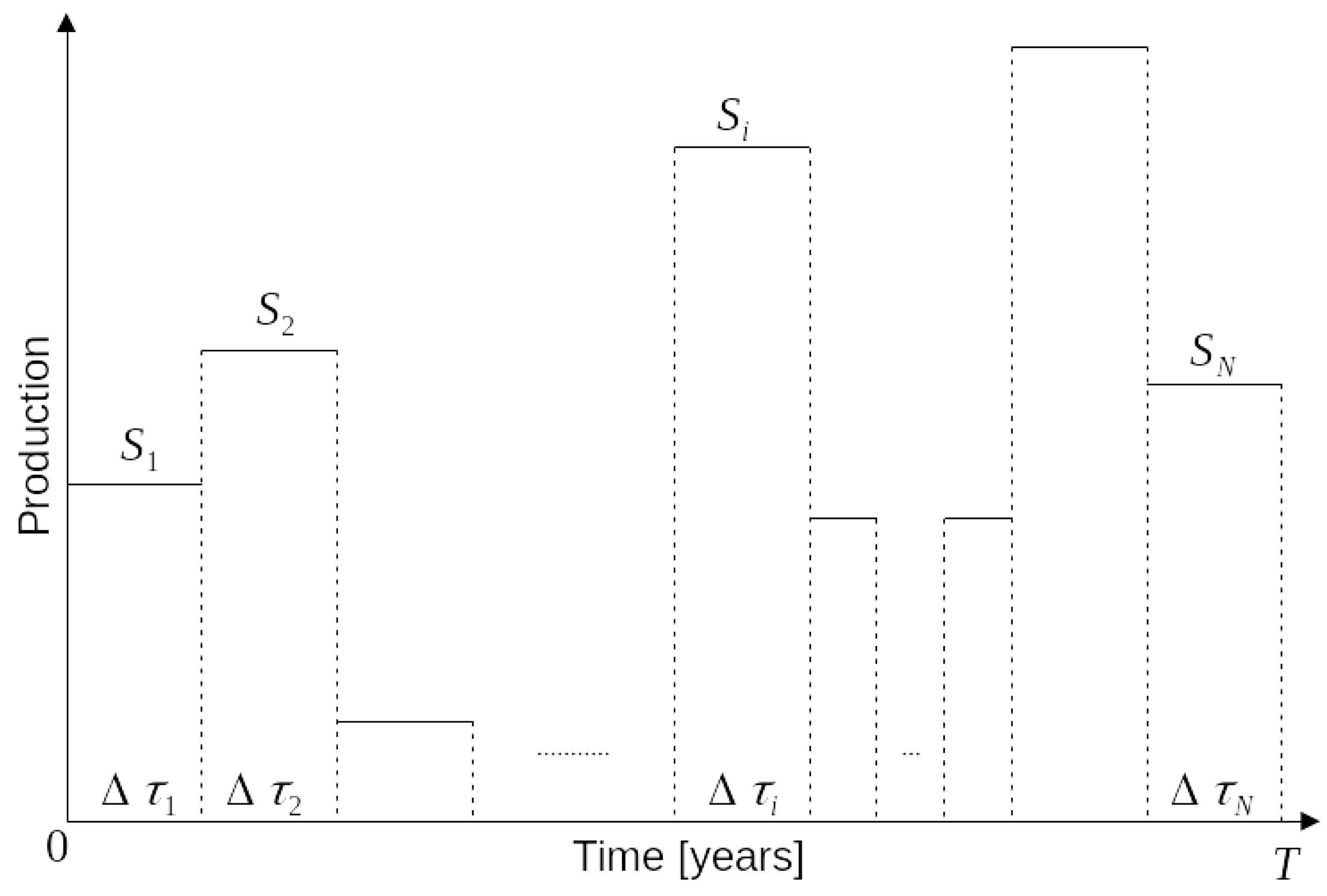
In order to reflect the actual operation of renewable energy sources (RES), a universal model must take into account not only electricity production but also the time shifts as well as RES downtimes. Figure 1 shows the actual course of the operation of RES in all T years of their operation using the staircase function. The revenues S from the sale of the electricity they generate are therefore, obviously, randomly distributed over years .
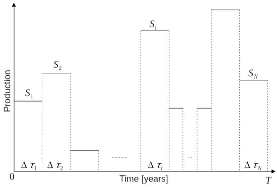
Figure 1.
The staircase function of the actual operation course of a renewable energy source (RES) in all T years of its operation.
For this actual curve, the total discounted net profit NPV should be determined (Formula (1)). Other measures of RES operation economic viability, such as IRR, DPBP, Break-Even Point (BEP), unit cost of electricity production , RES market value, market value supplied with electricity by RES, etc., are derivatives of the NPV measure [20,23,24,25,26,27,28]. Therefore, this makes it easier to develop nomograms of the economic viability for RES operation.
Obviously, only the electric power , the value of revenues S, operating costs , and discounted financial outlays for the construction of renewable energy sources are sufficient as input quantities for the construction of the universal NPV mathematical profit model. These are the quantities that characterise their economic efficiency. In addition, this model should take into account the interest rate r of the investment capital . Then, in multi-variant calculations, a wide range of values of these quantities, as well as the relations between them, should be used, which will allow us to prepare universal nomograms, thanks to which it will be possible to immediately determine the economic efficiency of the RES operation.
2.1. The General form of the Formula for Profit NPV from Operating a Renewable Energy Source (RES)
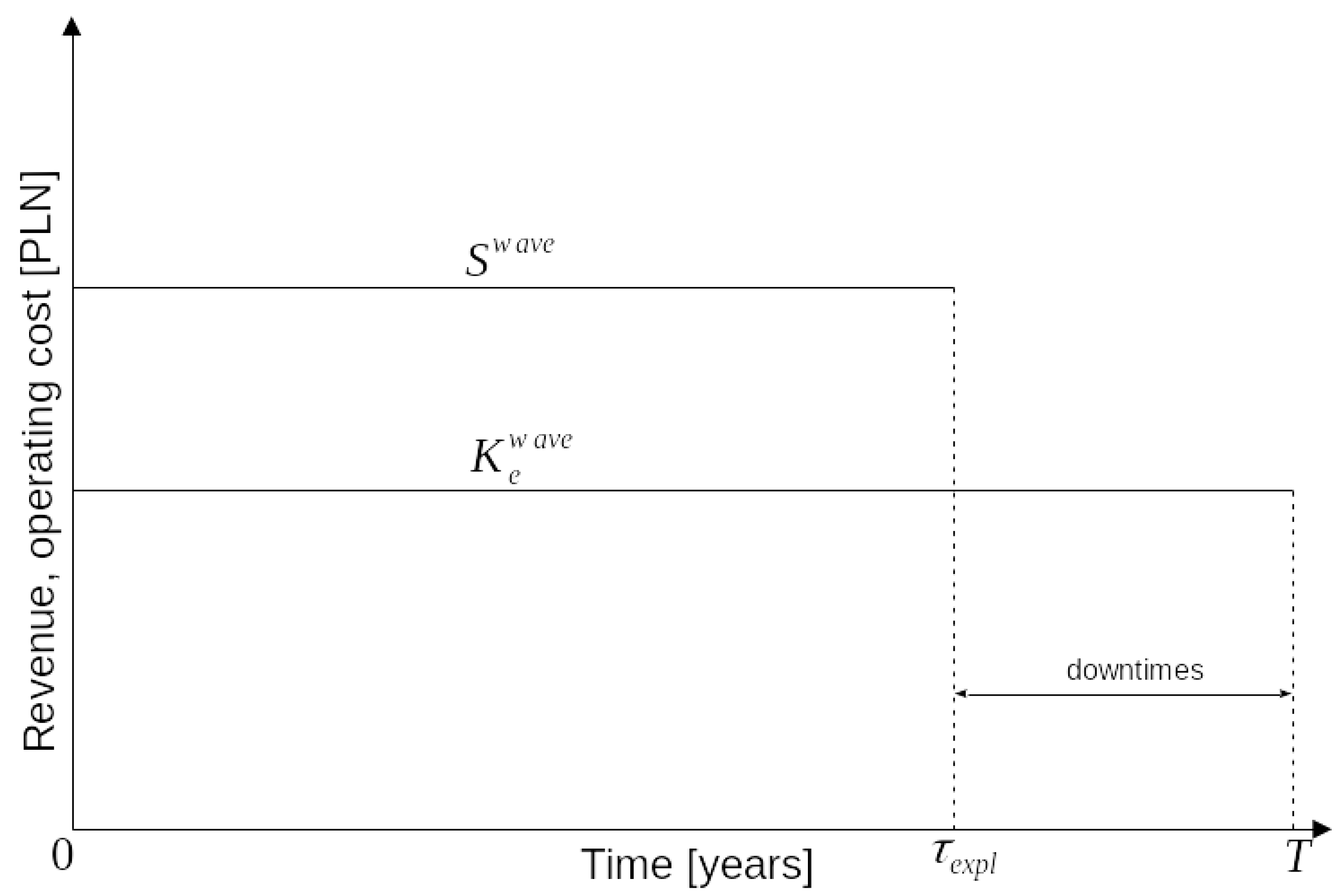
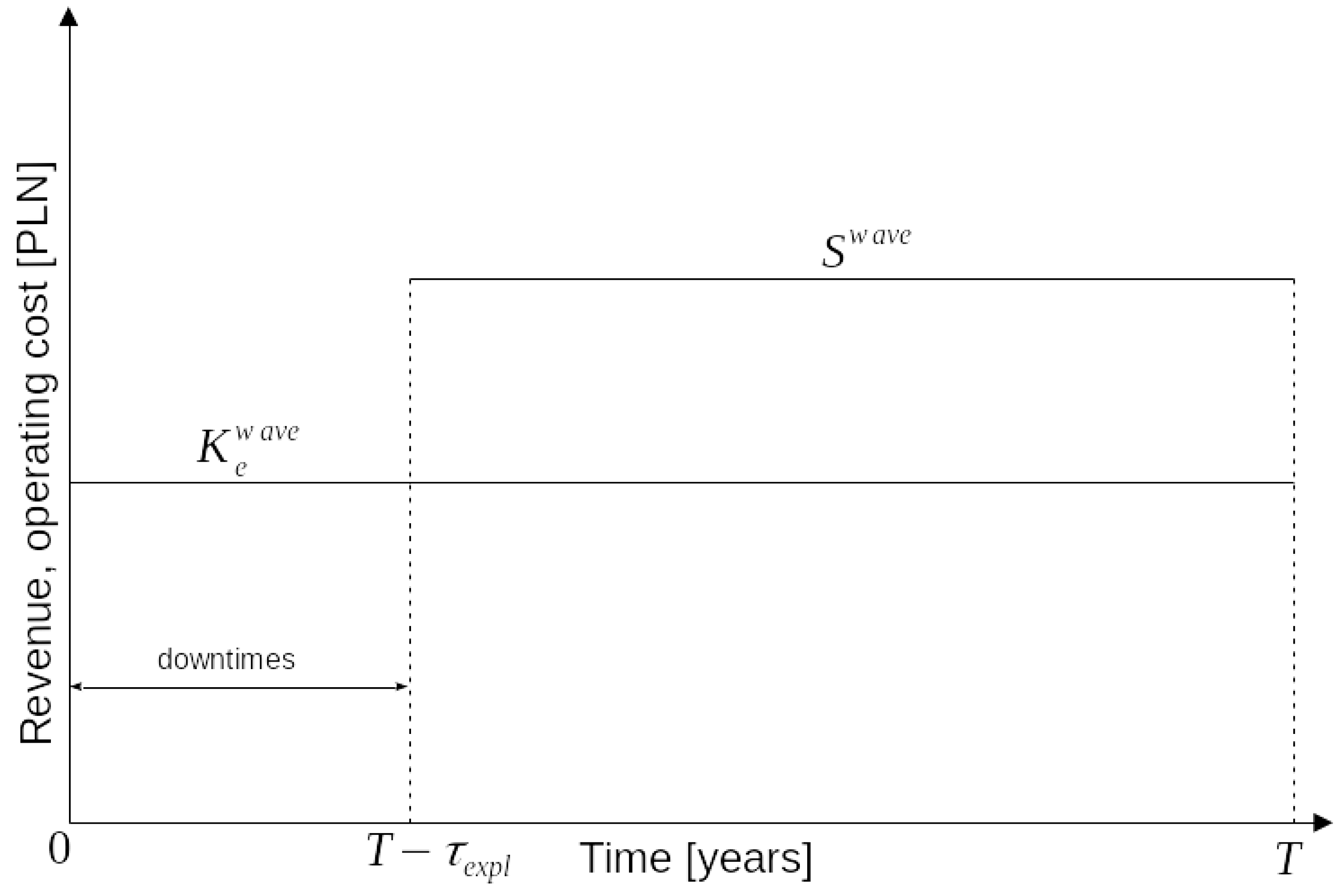
Figure 2 presents the general cumulative course of the weighted average operating costs and revenues from sales of electricity produced in an RES. It was prepared on the base of the actual staircase RES operation course shown in Figure 1. The extreme courses, i.e., the most favourable and the least economically advantageous, are presented in Figure 3 and Figure 4.
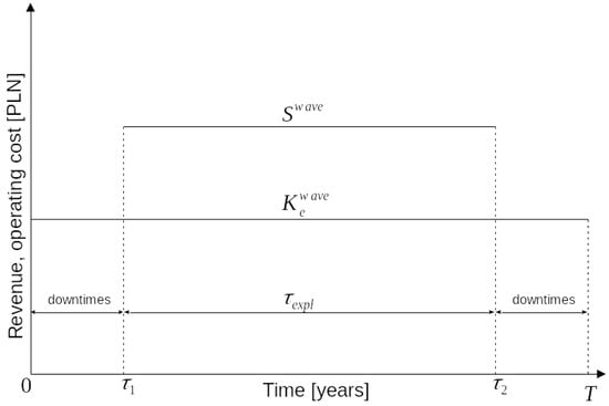
Figure 2.
Time course of the weighted average operating costs and revenues gained from renewable energy sources (RES).
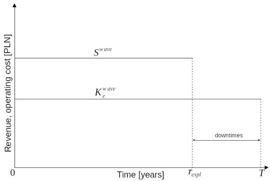
Figure 3.
Time-dependent course for the weighted average revenues and the costs of RES operation for the hypothetically most advantageous variant of their operation.

Figure 4.
Time-dependent course for the weighted average revenues and the costs of RES operation for the hypothetically least advantageous variant of their operation.
The maximum value of years is , minimum . If , then it is the most economically advantageous course of the actual RES operation from Figure 1 (Section 2.1.1). The least favourable course is if (Section 2.1.2). If, on the other hand, , then the intervals of years of production downtimes and are equal, and it can be assumed that if it is not the most likely RES work flow in years T, then it is the most likely, and thus the unit cost of electricity production in RES (Formula (15)) takes the values closest to the most probable ones.
The general form of the total discounted net profit NPV achieved in the range of years can be expressed in the continuous notation [28] according to Figure 1. Compare with Formulas (18) and (22):
where:
- —backward discounting factor;
- —cost of operation averaged over the time interval resulting from the staircase function of RES operation (time-varying operating costs together with capital costs are of course borne in all years T, hence also in those where revenues S from the sale of electricity are equal to zero, Figure 1);
- —income tax rate for gross profit;
- —the interest rate on investment capital (calculations assumed );
- —subsidy to a renewable energy source (RES) from the State Treasury (subsidies should not take place, they are used by individuals, and all taxpayers must contribute);
- —weighted average revenue resulting from the staircase function of revenues from a renewable energy source (RES) operation where the revenue is different from zero, ); Figure 1:
- —time;
- —total years of downtime, when renewable energy sources (RES) generate only operating and capital costs;
- —number of full years of renewable energy sources (RES) operation (turbine set or photovoltaic cell), i.e., when the wind turbine set (photovoltaic cell) works during T years of its operation for 8760 h/year, i.e., the years when renewable energy sources (RES) generate electricity sales revenue (Figure 1, Figure 2 and Figure 3):
- —annual RES operation ratio:
- —number of hours per year when renewable energy sources (RES) generate income from electricity sales (in Polish conditions, the annual operating time of a wind turbine set is only , while a solar cell operating time is );
- 8760
- —the number of hours per year (8760 = 365 days × 24 h),where for renewable energy sources (RES):where:
- —electricity sales price;
- —a subsidy from the State Treasury for each electric energy megawatt hour generated in a renewable energy source (RES);
- —gross electric power of a renewable energy source (RES);
- —the rate of fixed costs dependent on capital outlays (maintenance and repairs costs as well as payroll and insurance; the calculations assumed );
- —relative rate for the RES own needs of electricity (the calculations assumed ).
Interest (financial cost) F on the discounted investment capital and instalment R of its repayment (the sum of is the annual capital cost of RES operation; of course, the sum of the annual capital costs and annual operating costs is the annual RES operating costs , ) are expressed by the formulas [23,28]:
- Financial cost (interest on investment capital ):
- Instalment of investment capital repayment :
The investment outlays discounted at the moment of starting the renewable energy sources (RES) operation are expressed by the formula [23,28]:
where:
- —the coefficient of freezing the investment capital J during the b years of RES construction is [23,28] (the calculations assumed year):
The investment outlays J are represented by the equation:
where the unit investment outlays (per unit of power) for wind turbine sets and photovoltaic cells built on land are described by the dependence:
while power in (12) and (13) is expressed in megawatts (MW).
After substituting Equations (8) and (9) to Formula (1), and after performing the integration operation, the following is obtained:
From Formula (14), assuming that , the unit cost of electricity production in RES is calculated (Formula (15)). Then, in Formula (6), the price of electricity should be substituted with cost . Obviously, the lowest unit cost, i.e., , is when and the highest, i.e., , when .
From Formula (15), assuming that , the maximum subsidy from the State Treasury is calculated for each megawatt hour of electricity produced in RES. Then, in Formula (15), the dependence should be substituted with:
and then:
2.1.1. The Highest Achievable Profit from Operating a Renewable Power Source (RES)
Figure 3 presents the hypothetically most advantageous economical course of the actual operation of renewable energy sources (RES) from Figure 1. This is because it illustrates the highest possible profit from their operation (Formulas (18) and (19)). It is the case because all annual revenues with a weighted average value are accumulated in the range of years —Figure 3—and therefore, in Formula (14), the factor discounting revenues backwards for the moment 0 reaches its top level. In practice, the annual revenues of S are randomly distributed in years —Figure 1—while profit NPV from the use of RES, as already mentioned above, takes the value intermediate between profits and (see Formulas (19) and (23)).
The total maximum discounted net profit achieved in the entire range of years of RES operation is determined from the following equation (see Formula (1)):
After substituting Equations (8) and (9) to Formula (18), and after performing the integration operation, the following is obtained:
Formula (19), of course, can also be obtained from Formula (14), when time is substituted with value .
Of course, the condition is used to calculate the lowest unit cost of electricity production in RES. There are obvious relationships between values NPV and and (Formula (15)) and :
2.1.2. The Lowest Achievable Profit from Operating a Renewable Power Source (RES)
Hypothetically, the least economically advantageous work flow of renewable energy sources (RES) is presented in Figure 4. In this situation, the lowest possible profit from its operation is possible to achieve (Formulas (22) and (23)). This is due to the accumulation of annual RES revenues only in the last years of its operation —Figure 4—as a result of which, in Formula (23), the factor discounting revenues back to the moment 0 is the lowest.
The total discounted net profit achieved in the range of years of RES operation is then expressed by the equation (compare with Formulas (1) and (18)):
After integration, the following is obtained:
Formula (23), of course, can also be obtained from Formula (14), when time is substituted with value , and time is substituted with value .
Of course, the condition is used to calculate the highest unit cost of electricity production in RES. There are obvious relationships between values NPV and as well as and :
The variant in Figure 4, similarly to Figure 3, is obviously a theoretical variant with no practical significance. However, it had to be shown in order to compare the economical results obtained for it, along with the results for the most favourable variant presented in Section 2.1. Both these results represent extreme values for the actual course of the RES operation presented in Figure 1 and Figure 2.
3. Universal Charts of Unit Costs of Electricity Production in RES
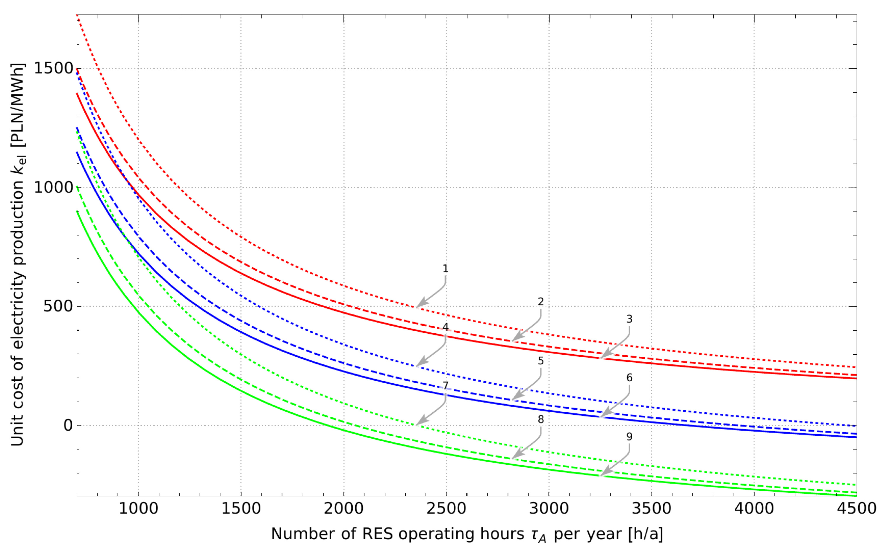
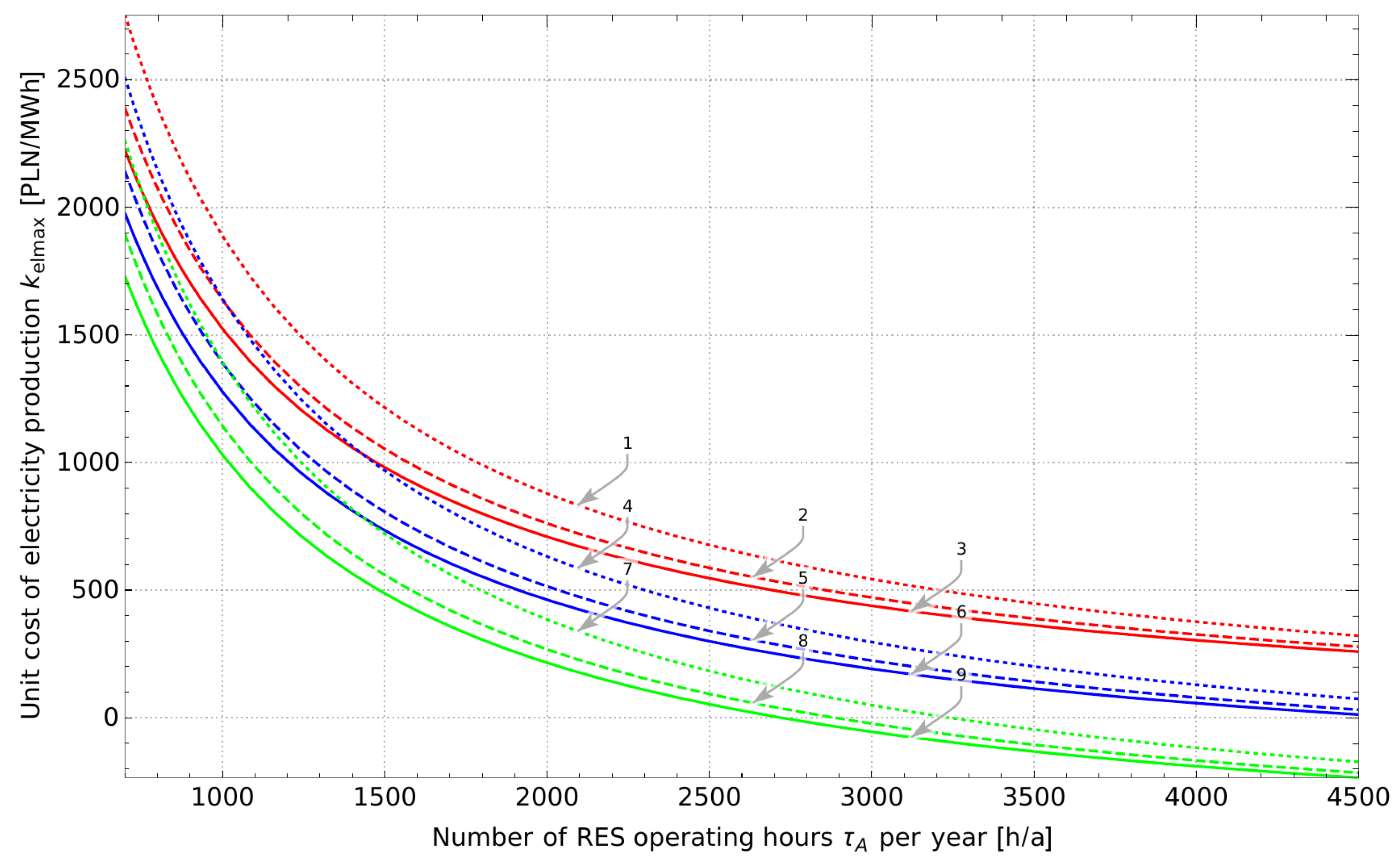
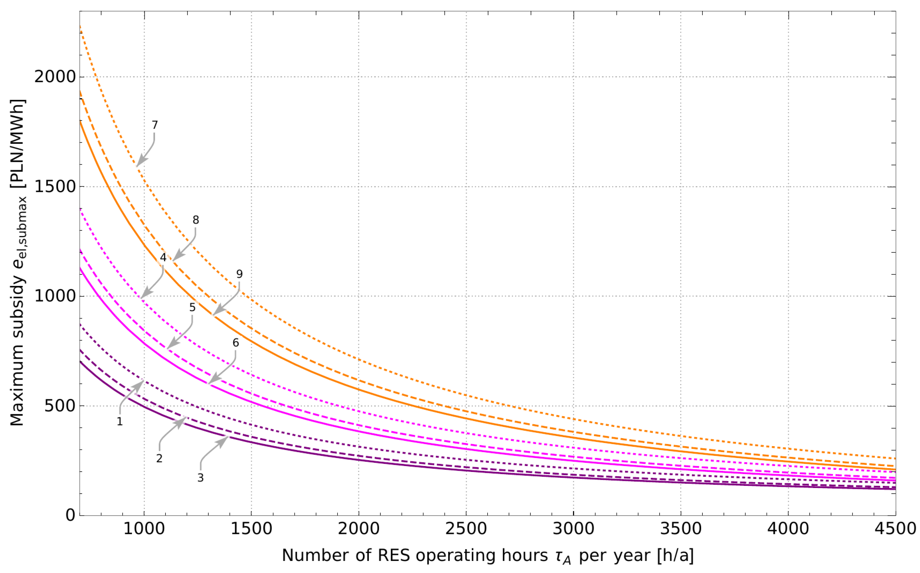
Figure 5, Figure 6 and Figure 7 show the values of the unit costs of electricity production in RES, and Figure 8 shows the values of the maximum subsidies from the State Treasury for each megawatt hour of electricity generated in RES, i.e., values , for which the unit cost is zero, .
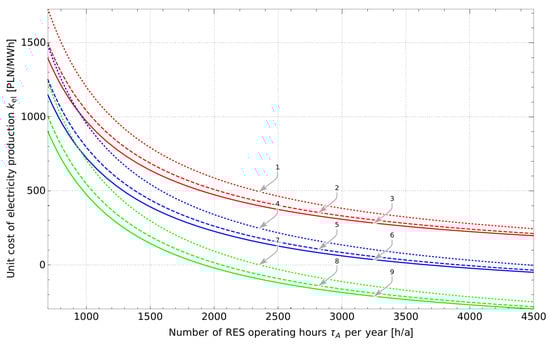
Figure 5.
Unit cost of electricity production as a function of time for
(1—, ; 2—, ;
3—, ; 4—, ;
5—, ; 6—; 7—, ; 8—; 9—, ).
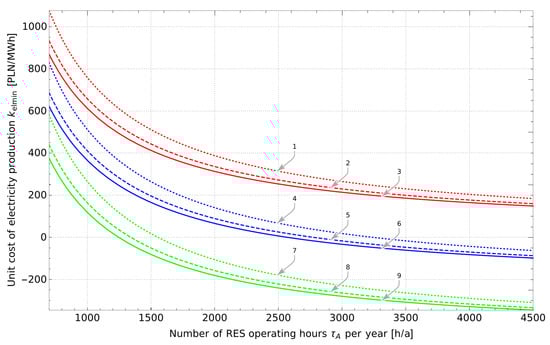
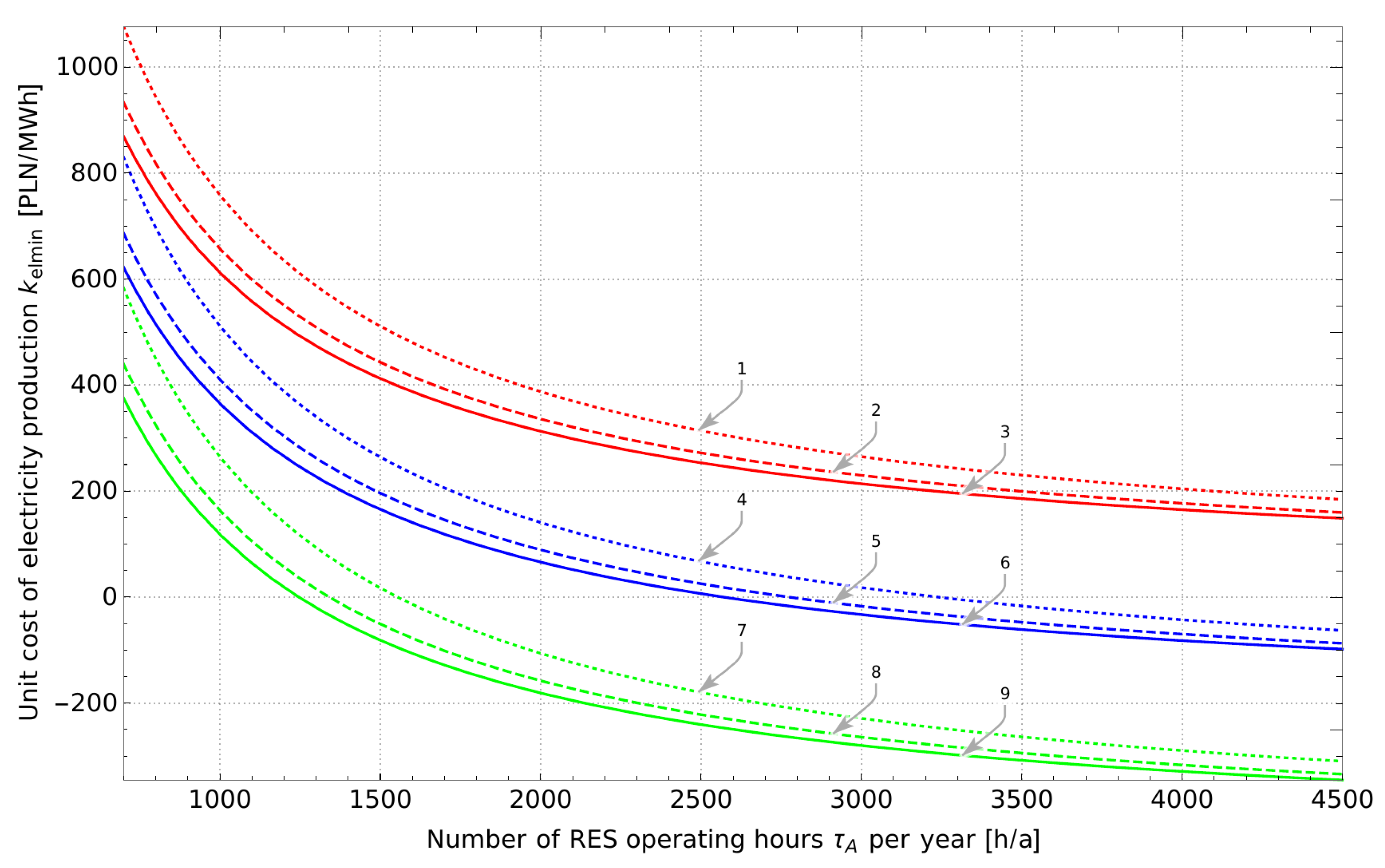
Figure 6.
Unit cost of electricity production as a function of time for (1—, ; 2—, ; 3—, ; 4—, ; 5—, ; 6—; 7—, ; 8—; 9—, ).
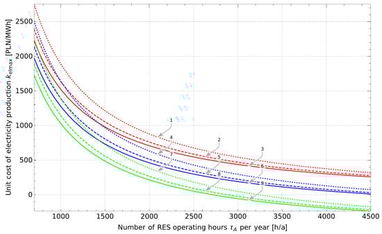
Figure 7.
Unit cost of electricity production as a function of time for (1—, ; 2—, ; 3—, ; 4—, ; 5—, ; 6—; 7—, ; 8—; 9—, ).
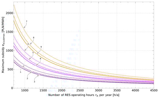
Figure 8.
Maximum subsidy as a function of time , (1—, ; 2—, ; 3—, ; 4—, ; 5—, ; 6—; 7—, ; 8—, ; 9—, ).
Figure 5 shows the unit cost for the situation where the number of years (Figure 2) takes the following value: . Then, the intervals of years of production downtime and are therefore equal, and thus the years of RES operation are symmetrically located in the interval of years —Figure 2. Of course, the values of these intervals change with the change in the number of hours of RES operation per year. The higher the value , the greater the number of complete years (Formula (3)) and thus the intervals and are smaller. However, this does not change the fact that they remain equal and that the years are still symmetrically located. Importantly, it should be considered that the costs calculated then are the most probable, that they are real values, and if they are not, then they are the closest to them.
As shown in Figure 5, the real unit cost of electricity production (i.e., with zero subsidy, of course ; curves 1, 2, 3) for real values of the number of hours , i.e., for values lower than 1500 h/a, is very high, much above PLN 600 /MWh. Therefore, it is several times higher than the costs obtained for all other energy technologies [28]. For example, for photovoltaic cells with power (curve 1 in Figure 5) for real time , this cost is as high as . Therefore, in order for RES to exist on the energy market, subsidies from the State Treasury are necessary for each megawatt hour of electricity produced there. Obviously, the greater the number of renewable energy operating hours per year, the lower subsidies should be given—Figure 8. For relatively high values and high values of subsidies , the costs in Figure 5 are negative. For example, for curve No. 9 ( ), this is the case for values . This results from the fact that the required maximum subsidies for and at (curve No. 6) presented in Figure 8 are lower than the values , for which curve 9 in Figure 5 was drawn up. The negative costs for RES owners are extremely beneficial, as they already have subsidies for the electricity they generate, with an excess paid from taxpayers’ pockets. Therefore, if they gave energy to the power grid even for free, they would make profits anyway. Of course, this is not the case, and although they sell it at a price of, for example, only about PLN 200/MWh, i.e., at a price even significantly below the cost of its production for any other energy technology, they gain enormous annual profits. Therefore, this is because of subsidies that renewable energy is said to be cheap, which is not true (sic). Meanwhile, if it were not for subsidies, the energy from renewable energy sources, being many times more expensive than the energy generated in any other energy technology, would be absolutely unsaleable.
Figure 6 shows the value of the unit cost of electricity production for the most economically advantageous (in fact unreal) work flow of renewable energy source (RES), presented in Figure 3, i.e., when the number of years is . So it is the minimum cost value, . Figure 7 shows the value of the unit cost for the least favourable course (also unreal) shown in Figure 4, i.e., when the cost has the highest value, . It should be noted that despite the fact that the values are unreal, they should be presented as they show significant cognitive values. They are the extreme values for the most likely value of the unit cost of electricity production in RES presented in Figure 5.
4. Summary and Final Conclusions
In conclusion, it should be expressly stated that the unit cost of electricity generation in renewable energy sources (RES), due to the very high unit costs (per unit of power, see Formula (13)) of investment outlays (equal to the outlays on power plants with supercritical parameters of live steam) and their very short annual operation times, is very high. It is many times higher than the costs obtained for any other available energy technologies [28]. The annual operating time of wind turbine sets in Poland is approx. 1500 h, while the time for photovoltaic cells is only approx. 750 h (in Germany, the annual use of wind turbine sets does not exceed 1400 h, photovoltaic cells 900 h [29]; it should be noted that the year has 8760 h). Only at sea and high in the mountains, the operating time of wind turbine sets is longer, even more than twice. However, then one should take into account significantly higher, even several times higher, unit investment outlays as compared with ‘land’ outlays equal to approx. 1.5 €/W—see Formula (13). The outlays for offshore turbine sets range from approx. 4 to approx. 7 €/W [30]. Therefore, they are even significantly higher than the outlays amounting to approx. €/W for nuclear power plants, where Rankine cycle is used. Such high outlays, despite significantly longer annual operating times, mean that offshore turbine sets do not make economical sense to an even greater extent than the ‘onshore’ ones.
Summing up, the production of electricity from RES, both onshore and offshore, is a solution that is not able to ensure sufficient, continuous, and stable electricity supplies throughout the year. Renewable energy sources (RES) are able to ensure its supply for a bit more than one hundred hours a month throughout a year on average, with very high unit costs and, as already mentioned, showing the absolute unpredictability of those supplies in time. Considering the above-mentioned fact, in order for electricity from renewable energy sources (RES) to exist on the electricity market, several tens of billions in annual subsidies from the State Treasury are required. For example, in Germany a few years ago, these subsidies amounted to €30 billion (sic) annually, while the installed wind turbine set capacity was 36,000 MW, and the value for photovoltaic power plant was 38,000 MW (subsidies for each megawatt hour of electricity generated by wind turbine sets amounted to €160, while by photovoltaic sources €430; currently in Germany, the power of turbine sets are already 56 GW). In Poland, from 2006 to 2020, subsidies amounted to PLN 76 billion, while currently they amount to over PLN 10 billion annually [29].
Author Contributions
Conceptualization, R.B.; methodology, R.B. and D.P.; software, R.B. and D.P.; validation, R.B. and D.P.; formal analysis, R.B. and D.P.; investigation, R.B. and D.P.; resources, R.B. and D.P.; data curation, R.B. and D.P.; writing—original draft preparation, R.B. and D.P.; writing—review and editing, R.B. and D.P.; visualization, D.P.; supervision, R.B.; project administration, R.B. and D.P. All authors have read and agreed to the published version of the manuscript.
Funding
This research received no external funding. The APC was funded by Opole University of Technology, Poland.
Conflicts of Interest
The authors declare no conflict of interest.
Abbreviations
| RES | Renewable Energy Sources |
| NPV | Net Present Value |
| IRR | Internal Rate of Return |
| DPBP | Discounted Pay Back Period |
| BEP | Break-Even Point |
References
- Li, J.; Wang, J. Forcasting of energy futures market and synchronization based on stochastic gated recurrent unit model. Energy 2020, 213, 118787. [Google Scholar] [CrossRef]
- Liu, L.; Wu, L. Forecasting the renewable energy consumption of the European countries by an adjacent non-homogeneous grey model. Appl. Math. Model. 2021, 89, 1932–1948. [Google Scholar] [CrossRef]
- Keeley, A.R.; Matsumoto, K.; Tanaka, K.; Sugiawan, Y.; Managi, S. The Impact of Renewable Energy Generation on the Spot Market Price in Germany: Ex-Post Analysis using Boosting Method. Energy J. 2020, 41. [Google Scholar] [CrossRef]
- Nguyen, J.; Valadkhani, A.; Hajargasht, G. The Choice between Renewables and Non-renewables: Evidence from Electricity Generation in 29 Countries. Energy J. 2021, 42. [Google Scholar] [CrossRef]
- Hussain, J.; Zhou, K.; Muhammad, F.; Khan, D.; Khan, A.; Ali, N.; Akhtar, R. Renewable energy investment and governance in countries along the Belt & Road Initiative: Does trade openness matter? Renew. Energy 2021, 180, 1278–1289. [Google Scholar] [CrossRef]
- Steffen, B. Estimating the cost of capital for renewable energy projects. Energy Econ. 2020, 88, 104783. [Google Scholar] [CrossRef]
- Shair, J.; Li, H.; Hu, J.; Xie, X. Power system stability issues, classifications and research prospects in the context of high-penetration of renewables and power electronics. Renew. Sustain. Energy Rev. 2021, 145, 111111. [Google Scholar] [CrossRef]
- D’Adamo, I.; Rosa, P. Current state of renewable energies performances in the European Union: A new reference framework. Energy Convers. Manag. 2016, 121, 84–92. [Google Scholar] [CrossRef]
- Özge, Ö.; Hobbs, B.F.; van Hout, M.; Koutstaal, P.R. Capacity vs energy subsidies for promoting renewable investment: Benefits and costs for the EU power market. Energy Policy 2020, 137, 111166. [Google Scholar] [CrossRef]
- Helm, C.; Mier, M. Steering the energy transition in a world of intermittent electricity supply: Optimal subsidies and taxes for renewables and storage. J. Environ. Econ. Manag. 2021, 109, 102497. [Google Scholar] [CrossRef]
- Meus, J.; De Vits, S.; S’heeren, N.; Delarue, E.; Proost, S. Renewable electricity support in perfect markets: Economic incentives under diverse subsidy instruments. Energy Econ. 2021, 94, 105066. [Google Scholar] [CrossRef]
- Goh, T.; Ang, B. Quantifying CO2 emission reductions from renewables and nuclear energy—Some paradoxes. Energy Policy 2018, 113, 651–662. [Google Scholar] [CrossRef]
- Duffy, A.; Hand, M.; Wiser, R.; Lantz, E.; Dalla Riva, A.; Berkhout, V.; Stenkvist, M.; Weir, D.; Lacal-Arántegui, R. Land-based wind energy cost trends in Germany, Denmark, Ireland, Norway, Sweden and the United States. Appl. Energy 2020, 277, 114777. [Google Scholar] [CrossRef]
- Rodrigo, P.; Gutiérrez, S.; Micheli, L.; Fernández, E.; Almonacid, F. Optimum cleaning schedule of photovoltaic systems based on levelised cost of energy and case study in central Mexico. Solar Energy 2020, 209, 11–20. [Google Scholar] [CrossRef]
- Zografidou, E.; Petridis, K.; Petridis, N.E.; Arabatzis, G. A financial approach to renewable energy production in Greece using goal programming. Renew. Energy 2017, 108, 37–51. [Google Scholar] [CrossRef] [Green Version]
- García-Gusano, D.; Espegren, K.; Lind, A.; Kirkengen, M. The role of the discount rates in energy systems optimisation models. Renew. Sustain. Energy Rev. 2016, 59, 56–72. [Google Scholar] [CrossRef]
- Nguyen, T.A.T.; Chou, S.Y. Improved maintenance optimization of offshore wind systems considering effects of government subsidies, lost production and discounted cost model. Energy 2019, 187, 115909. [Google Scholar] [CrossRef]
- Lee, B.; Lim, D.; Lee, H.; Byun, M.; Lim, H. Techno-economic analysis of H2 energy storage system based on renewable energy certificate. Renew. Energy 2021, 167, 91–98. [Google Scholar] [CrossRef]
- Antony, A.; Maheshwari, N.; Rao, A.R. A generic methodology to evaluate economics of hydrogen production using energy from nuclear power plants. Int. J. Hydrog. Energy 2017, 42, 25813–25823. [Google Scholar] [CrossRef]
- Bartnik, R.; Buryn, Z.; Hnydiuk-Stefan, A. Investment Strategy in Heating and CHP. Mathematical Models; Springer: Cham, Switzerland, 2017. [Google Scholar] [CrossRef]
- Hara, K. Characterization of stationary preferences in a continuous time framework. J. Math. Econ. 2016, 63, 34–43. [Google Scholar] [CrossRef]
- Bartnik, R.; Buryn, Z.; Hnydiuk-Stefan, A. Methodology and mathematical model with the continuous time for the selection of the optimal power of the gas turbine set for the dual fuel gas-steam combined cycle in a parallel system. Appl. Therm. Eng. 2018, 141, 1161–1172. [Google Scholar] [CrossRef]
- Bartnik, R.; Bartnik, B. Economic Account in Power Engineering; WNT: Warsaw, Poland, 2014. (In Polish) [Google Scholar]
- Bartnik, R.; Bartnik, B. Mathematical model of optimum investment strategy search in power industry. Energetyka 2015, 1, 16–20. (In Polish) [Google Scholar]
- Bartnik, R.; Bartnik, B. Mathematic models with continuous time analysis and determination of heat and electric energy market value as well as of power stations and CHP plants. Energetyka 2015, 7, 450–456. (In Polish) [Google Scholar]
- Bartnik, R. A search for an optimum investment strategy in power industry. Methodology and results of sample calculations. Energetyka 2015, 10, 627–631. (In Polish) [Google Scholar]
- Bartnik, R. Measures and mathematical models in continuous time recording of economic efficiency analysis for power industry investments, valuation of heat and electricity market fair value and a market value of power companies. Energetyka 2016, 8, 440–445. (In Polish) [Google Scholar]
- Bartnik, R.; Buryn, Z.; Hnydiuk-Stefan, A. Economics of Power Engineering in Mathematical Models with Continuous Time; PWN: Warsaw, Poland, 2017. (In Polish) [Google Scholar]
- Chmielewski, A.; Smoliński, T. Energy policy of selected European countries, role of nuclear energy. Instal 2015, 2, 12–18. (In Polish) [Google Scholar]
- Majcher, J. On the superiority of one holiday over another, or RES vs nuclear power. Nowa Energia 2021, 1, 58–61. (In Polish) [Google Scholar]

Publisher’s Note: MDPI stays neutral with regard to jurisdictional claims in published maps and institutional affiliations. |
© 2021 by the authors. Licensee MDPI, Basel, Switzerland. This article is an open access article distributed under the terms and conditions of the Creative Commons Attribution (CC BY) license (https://creativecommons.org/licenses/by/4.0/).