MPPT Improvement for PMSG-Based Wind Turbines Using Extended Kalman Filter and Fuzzy Control System

Abstract

Variable speed wind turbines are commonly used as wind power generation systems because of their lower maintenance cost and flexible speed control. The optimum output power for a wind turbine can be extracted using maximum power point tracking (MPPT) strategies. However, unpredictable parameters, such as wind speed and air density could affect the accuracy of the MPPT methods, especially during the wind speed small oscillations. In this paper, in a permanent magnet synchronous generator (PMSG), the MPPT is implemented by determining the uncertainty of the unpredictable parameters using the extended Kalman filter (EKF). Also, the generator speed is controlled by employing a fuzzy logic control (FLC) system. This study aims at minimizing the effects of unpredictable parameters on the MPPT of the PMSG system. The simulation results represent an improvement in MPPT accuracy and output power efficiency.

1. Introduction

To keep the earth safe and deal with potential environmental threats, sustainable and pollution-free technologies have been introduced, known as renewable energy technologies (RETs). Energy sources can be divided into three main categories: (i) fossil fuels, (ii) nuclear energy, and (iii) renewable energies [1]. Renewable energy sources (RESs) refer to the types of energy that, unlike non-renewable energies, can be re-created or renewed by nature in a short period [2]. The leading types of renewable energies are solar [3,4], wind [5], geothermal [6,7], marine energy [8], biomass [9], and biofuels [10,11]. RESs can provide zero or almost zero percent pollution. RETs are reliable, cost-effective, and environmentally friendly methods to meet the energy requirements of rural areas on a small scale.

The first wind turbine for electricity generation was developed at the end of the 19th century (1887–1888) when Brush built the first automatically operating wind turbine with 12 kW [12]. Nowadays, the contribution of wind turbines in the production of electrical energy has been significantly increased. Efficient control strategies are necessary to improve the wind turbines’ performance and reduce operation and maintenance costs. The maximum power point tracking (MPPT) method is crucial in extracting the optimum wind output power. Designing MPPT strategies requires a model that includes mechanical and electrical components based on the accurate examination of wind turbine conditions. This model contains some unpredictable parameters which could affect the accuracy of MPPT methods. The uncertainty of these parameters brings more speed oscillations and power fluctuations [13].

In the current literature, many studies have focused on wind turbine control and output power optimization. Various strategies have been developed for pitch control schemes which have used PID controllers [14], linear quadratic Gaussian (LQG) controller [15], reliable control [16], gain scheduling [17], periodic disturbance accommodating control [18], fuzzy logic control (FLC) [19], and linear parameter-varying (LPV) control methods [20].

Richie Gao and Zhiwei Gao [14] proposed a novel PI-based pitch control technique employing direct search optimization, delay perturbation estimation, and signal compensation to overcome the shortcomings caused by hydraulic driven units, such as unknown delays. Although no prior delay is necessary for the proposed method, the introduced method increases the complexity of the control system. Najafi-Shad et al. [21] introduced a novel MPPT method for hybrid PV-wind turbine generation systems by reducing the number of power system converters. This intelligent MPPT method can decrease the generated power in over-rating conditions, decreasing the power and voltage fluctuations. Gliga et al. [22] have proposed a novel fault diagnosis and identification method for eccentricity faults in a PMSG-based wind turbine using EKF and Fast Fourier Transform (FFT). Although employing the introduced method spectrum of the stator currents is invariant to changes in the wind speed, it is sensitive to faults and affects the system output power. Using the ensemble Kalman filter (EnKF), Afrasiabi et al. [23] introduces a nonlinear static state estimation for the PMSG wind turbine. The results of this study are compared with the unscented Kalman filter (UKF) and EKF. Zhang [24] has introduced a novel control method for power system converters in a grid-connected PMSG-based wind turbine structure by employing predictive controllers and state estimators. The introduced method has acceptable performances at different wind speeds and load situations. However, it needs parameter tuning efforts. In order to compensate for the effect of the incomplete dynamic equation for the estimations of induction motor parameters, Zerdali [25] proposes designing an adaptive fading EKF (AFEKF) observer. To show the superiority of AFEKF, its estimation performance is compared to that of standard EKF methods, especially in transient states. However, the introduced observer is sensitive to the variations caused by temperature and frequency changes and should be updated continuously. Bagheri [26] introduces a new independent approach of external factors for eccentricity fault detection and discrimination in induction motors and estimates the exact severities of the faulty components using an unscented Kalman–Bucy filter (UKBF), which shows efficient performance in different types of eccentricity faults. Ortatepe and Karaarslan [27] have proposed the employment of a reduced-order EKF instead of the full-order EKF in a DFIG-based wind turbine to increase the system stability against variations of rotor and stator resistors. In this paper, a model predictive control method is used to provide easy implementation of the matrix converter, and in order to eliminate disadvantages of the model predictive control method, a reduced-order EKF has been applied as an observer to the reducing of the execution time of the algorithm.

The articles mentioned above have not taken a holistic approach in considering estimating the uncertainty of unpredictable parameters and improving the accuracy of the MPPT method. Instead, they concentrate on the PMSG state estimation and control structure.

This paper intends to introduce a generator speed and MPPT control system for wind turbines based on parameters’ estimation. In other words, in a PMSG-based wind turbine, the MPPT reference estimation is developed employing the EKF, and generator speed control is performed using the FLC. The simulation results verify the ability and effectiveness of the proposed MPPT method in comparison with conventional ones. In general, this study yields the following benefits:

• Improving the accuracy of the wind turbine MPPT implementation.
• Increasing the efficiency of the PMSG output power by estimating the generator speed.
• Estimating the unpredictable parameters by employing EKF in PMSG-based wind turbines to the best knowledge of the authors.

2. Proposed Method

In order to model the proposed MPPT fault reduction method, variable speed wind power generation systems, generator speed determination, and MPPT control must be identified to create a mathematical model. Compared to a fixed-speed wind turbine (FSWT), a VSWT can operate at a broader range of wind speeds. Also, VSWTs can generate 10 to 15 percent more energy than installed FSWTs and have less stress on mechanical components, especially blades and shafts, which results in less power fluctuation [28]. Since the wind velocity could change every moment, the MPPT method should track the small oscillations of generator speed and maximum power points. PMSGs and doubly fed induction generators (DFIGs) are typical VSWTs used for wind turbine configurations. Although DFIGs are more broadly used because of their ability to work at a more extensive speed range, the PMSG has such advantages as:

• The PMSG-based wind turbine is directly driven, which makes it easily controllable.
• This VSWT has a slow rotation speed.
• It has high torque density and very low inertia, which makes it highly efficient.
• This type of VSWTs can be used without the gearbox.

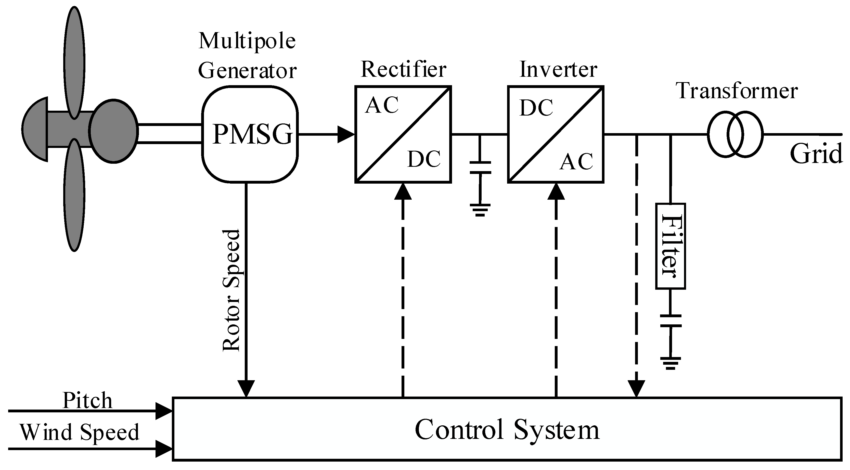
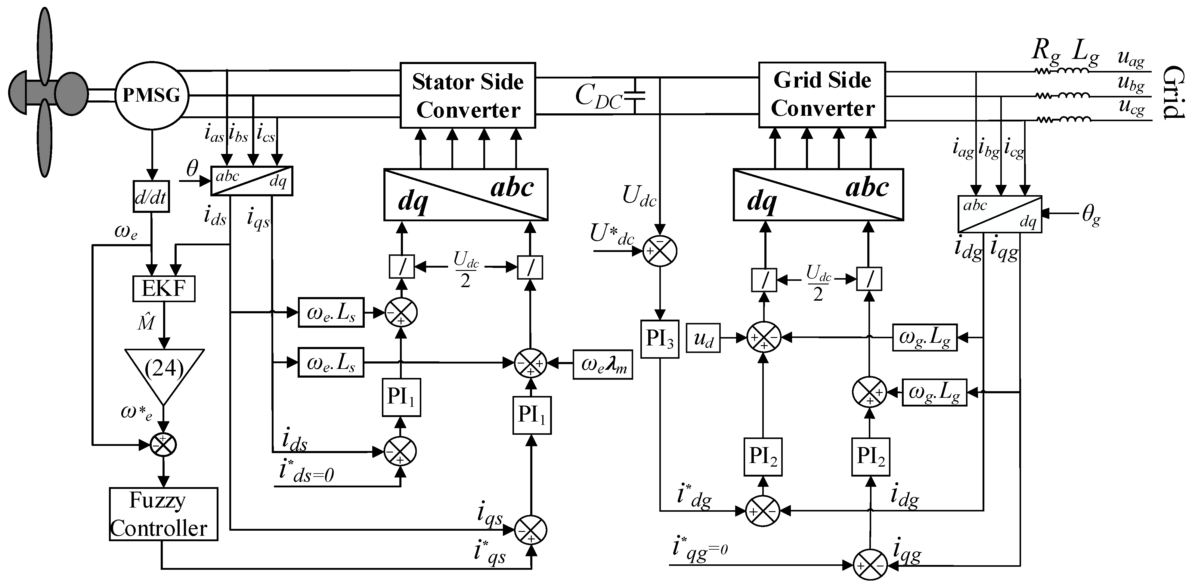
A typical PMSG configuration consists of blades, a generator, a control system, and power electronic converters. The generated electricity has variable frequency and voltage that cannot be directly injected into the grid. The generator is connected to a three-phase rectifier called a stator side converter (SSC), which rectifies the generator current to charge the DC-link capacitor and has primary duties consisting of MPPT, active and reactive power control, and DC-link voltage control [18]. The DC-link voltage feeds a three-phase inverter, called a grid side converter (GSC), connected to the grid through a transformer. Figure 1 shows the general wind turbine PMSG system with its control scheme.

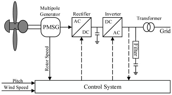
Figure 1. The general PMSG wind turbine system with its control schemes.

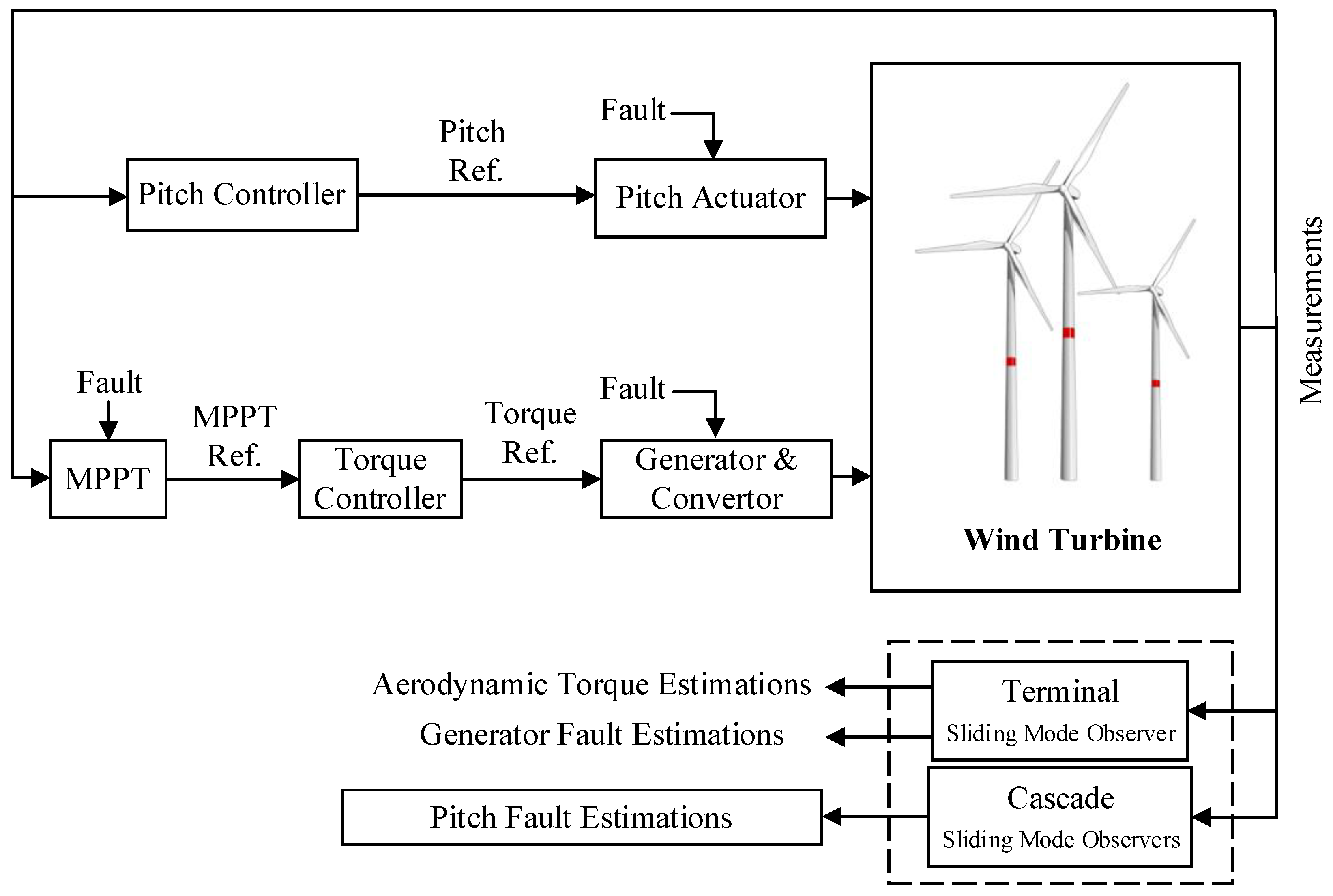
Numerous qualitative and quantitative studies have been proposed for estimating, diagnosing, and detecting faults. Also, geometric, observer-based, slip-state, robust, and adaptive estimation methods have been presented in the previous studies [29,30]. A typical block diagram of the wind turbine fault detection and diagnosis system is depicted in Figure 2.

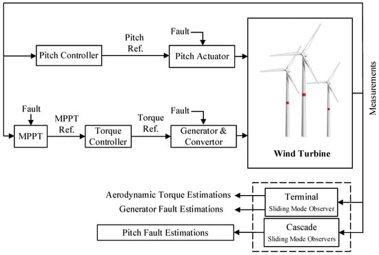
Figure 2. Fault diagnosis scheme block diagram.

One of the most common forms of wind turbine faults is the MPPT fault, which occurs during the small oscillations of wind speed. In other words, the uncertainty of variable parameters, such as wind speed and air density, could make the reference signal of the generator speed inaccurate, leading to the tracking of a wrong signal by the MPPT. The primary goal of this study is to minimize the MPPT fault of the PMSG-based wind turbine, especially during the small oscillations of the wind speed.

2.1. System Description

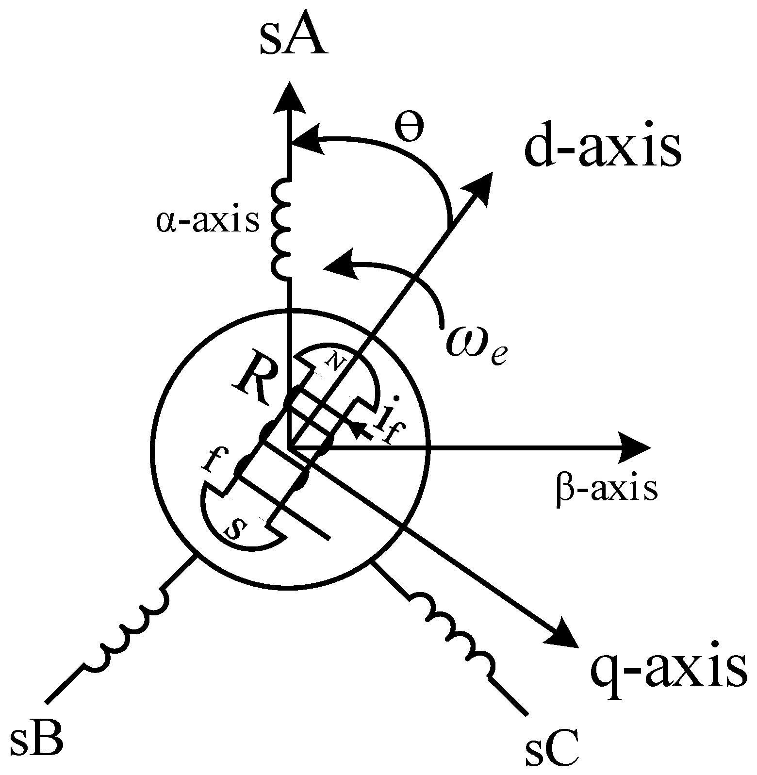
In order to control the PMSG in the proposed configuration, the voltage-flux equations in the d-q reference frame method are used, which provides independent control parameters and a simple design compared to other methods [31]. In this model, the d-axis of the frame is aligned with the rotor’s flux vector and rotates at synchronous speed. Figure 3 shows the proposed dp-coordinate frame of the PMSG.

Figure 3. The dq-coordinate frame of the PMSG.

2.1.1. SSC Control

The SSC control consists of two independent control loops. The first one controls the reference current i_ds at zero to achieve a unity power factor. The second one consists of two cascade loops, in which an outer loop is used to maximize power by setting the reference current i_qs for the inner current loop [31].

The SSC controls the stator terminal voltage components u_ds and u_qs. It performs this task through the sinusoidal pulse with modulation (PWM). The PMSG is modeled using Equations (1) and (2), based on stator current and voltages as follows [32]:

$$u_{ds}=R_s{i}_{ds}+L_s\frac{d{i}_{ds}}{dt}+{\omega }_e{L}_s{i}_{qs}$$

(1)

$$u_{qs}=R_s{i}_{qs}+L_s\frac{d{i}_{qs}}{dt}+{\omega }_e{L}_s{i}_{ds}+{\omega }_e{\lambda }_m$$

(2)

where the $u_{ds}$ and $u_{qs}$ are components of the stator voltage, the $i_{qs}$ and $i_{qs}$ are the stator current components. λ_m is core magnetic flux and, ${\omega }_e$ illustrates the rotor angular speed. Also, R_s and L_s show the stator resistance and inductance, respectively. The controller output voltage signals are obtained through the new variables $u_{sd}^{\prime }$ and $u_{sq}^{\prime }$ [31]:

$$m_{ds}=\frac{2}{U_{dc}} \left(u_{ds}^{\prime }-{\omega }_e{L}_s{i}_{qs}\right)$$

(3)

$$m_{qs}=\frac{2}{U_{dc}} \left(u_{qs}^{\prime }-{\omega }_e{L}_s{i}_{ds}+{\omega }_e{\lambda }_m\right)$$

(4)

where the $m_{ds}$ and $m_{qs}$ are the SSC modulation indexes, and U_dc shows the DC-link voltage. Based on Equations (3) and (4), the following transfer function can be extracted for both $i_{ds}$ and $i_{qs}$:

$$G_{ir}\left(s\right)=\frac{I_{qs}\left(s\right)}{U_{qs}^{\prime }\left(s\right)}=\frac{I_{ds}\left(s\right)}{U_{ds}^{\prime }\left(s\right)}=\frac{1}{L_s s+R_s}$$

(5)

A PI controller (PI1) is designed based on the zero-pole cancellation method to control the stator current components. Therefore, the plant transfer function pole should be at the zero of the controller. Moreover, to achieve an adequate bandwidth, the time constant of the closed-loop current control (TS) is selected to be one-tenth of the switching frequency of the SSC [21]. So, the parameters of PI1 controller are:

$$K_{ps}=\frac{L_s}{T_S}$$

(6)

$$K_{is}=\frac{R_s}{T_S}$$

(7)

2.1.2. GSC Control

Similar to the SSC control, the GSC control comprises two control loops. The first one controls the DC-link voltage, and the second one controls the d-component of the grid current i_dg. Also, the reactive power can be controlled at zero in order to achieve the unity power factor. The grid voltage components are as in Equations (8) and (9) [31].

$$u_{dg}=-(R_g{i}_{dg}+L_g\frac{d{i}_{dg}}{dt})-{\omega }_g{L}_g{i}_{qg}+u_d$$

(8)

$$u_{dg}=-(R_g{i}_{qg}+L_g\frac{d{i}_{qg}}{dt})-{\omega }_g{L}_g{i}_{dg}$$

(9)

where $R_g$ and $L_g$ are the grid side filter resistance and inductance. $u_d$ and ${\omega }_g$ are the d-component of the PCC voltage and network angular frequency, respectively. $u_{d,qg}$ and $i_{d,qg}$ are the GSC voltage and current components. The controller output voltage signals can be controlled through the new variables $u_{dg}^{\prime }$ and $u_{qg}^{\prime }$ [31]:

$$m_{dg}=\frac{2}{U_{dc}} \left(-u_{dg}^{\prime }-{\omega }_g{L}_g{i}_{qg}+u_d\right)$$

(10)

$$m_{qg}=\frac{2}{U_{dc}} \left(-u_{qg}^{\prime }-{\omega }_g{L}_g{i}_{dg}\right)$$

(11)

where the $m_{dg}$ and $m_{qg}$ are the SSC modulation indexes. To design the grid side current controllers (PI2), the same approach as the one used to design PI1 is employed. Therefore, the PI2 parameters are:

$$K_{pg}=\frac{L_g}{T_S}$$

(12)

$$K_{ig}=\frac{R_g}{T_S}$$

(13)

To design the outer loop controller (PI3), the power balance between the dc and ac sides of the GSC can be illustrated as [31]:

$$\frac{d{U}_{dc}}{dt}=\frac{1}{C{U}_{dc}}{P}_s-\frac{1}{C{U}_{dc}}{P}_g$$

(14)

where $P_s$ and $P_g$ are the stator output active power and active power delivered to the grid, respectively. In order to keep the DC-link voltage constant, the first part of Equation (14) should be zero. Thus, the stator output active power and the delivered power to the grid are equal. The following relationships are used to design the parameters of the PI3 controller [33]:

$$K_{pdc}=\frac{C}{4T_s }$$

(15)

$$K_{idc}=8T_s$$

(16)

2.2. Parameter Estimation

In this section, an estimation and control strategy for unpredictable parameters of the PMSG is introduced. First, the reference signal of generator speed is determined by estimating uncertain parameters through the EKF. Then, using the reference speed, the FLC is employed to design the q-component reference current of the stator.

Equations (1) and (2) show that the stator current components are not only affected by the $u_{sd}$ and $u_{sq}$ voltages, but also by the $-{\omega }_e{L}_s{i}_{sq}$,${\omega }_e{L}_s{i}_{sd}$, and ${\omega }_e{\lambda }_m$ voltages. These voltages are rotor speed functions and will increase substantially as the generator is operating at high speed. Under these conditions, the voltage components will affect the output torque of the current, and the output torque will be inaccurate. Therefore ${\omega }_e$ and $u_{sq}$ determine the EKF model. For wind turbines, wind power can be expressed as Equation (17) [34].

$$P_{wind}=\frac{1}{2}\rho A{V}_w^3$$

(17)

where $\rho$ is the air density, $A$ is the rotor swept area, and $V_w$ is the wind velocity. The mechanical power of the wind turbine extracted from the wind power is given as Equation (18) [34].

$$P_m=P_{wind}{C}_P\left(\theta ,\lambda \right)=\frac{1}{2}\rho A{C}_p\left(\theta ,\lambda \right)V_w^3$$

(18)

where $C_p\left(\theta ,\lambda \right)$ is called the performance coefficient and is a function of the pitch angle ($\theta$) and tip speed ratio $\left(\lambda \right)$. The tip speed ratio can be defined as Equation (19) [34].

$$\lambda =\frac{r\omega }{V_w}$$

(19)

where $r$ is the rotor radius, and $\omega$ is the blades’ angular velocity. A typical wind turbine performance coefficient example is specified as Equations (20) and (21) [34].

$$C_p=0.22\left(\frac{116}{{\lambda }_i}-0.4\theta -5\right)e^{\frac{-12.5}{{\lambda }_i}}$$

(20)

$${\lambda }_i=1/\left(\frac{1}{\lambda +0.08\theta }-\frac{0.035}{{\theta }^3+1}\right)$$

(21)

By replacing Equation (20) in Equation (21), the following extensive model can be derived:

$$C_p=0.22\left(\frac{116}{\lambda +0.08\theta }-\frac{4.06}{{\theta }^3+1}-0.4\theta -5\right)e^{-\left(\frac{12.5}{\lambda +0.08\theta }-\frac{0.4375}{{\theta }^3+1}\right)}$$

(22)

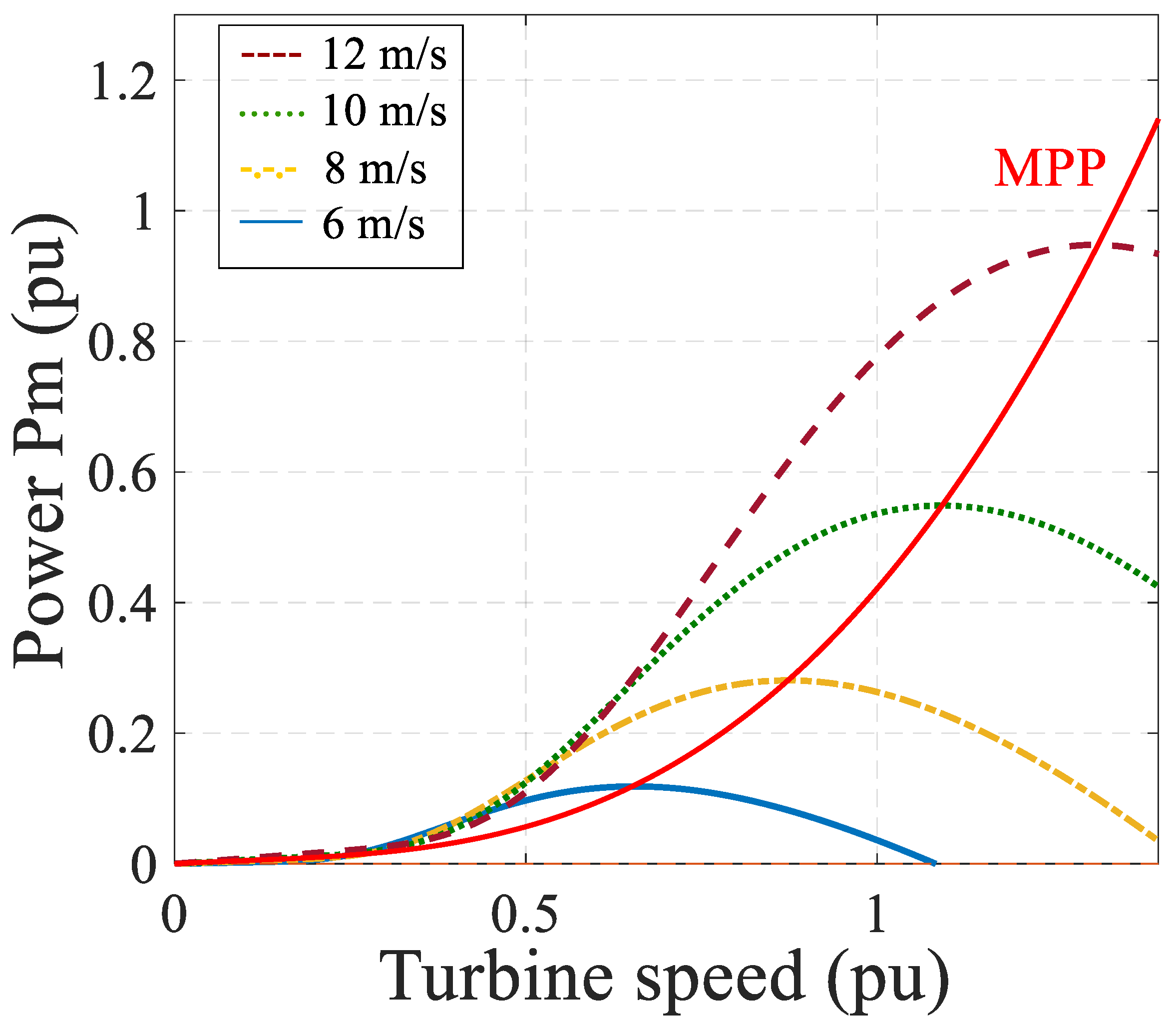
Generally, for small grid-connected wind turbines with a low capacity (less than 10 kW), $\theta$ will be constant. Therefore, the performance coefficient only depends on $\lambda$. The $P_m-\omega$ curves at different wind speeds are depicted in Figure 4.

Figure 4. $P_m-\omega$ curves at different wind speeds.

Figure 4 shows that at maximum power points at different wind speeds, the Equation (23) exists.

$$\frac{d{p}_m}{d\omega }=0$$

(23)

This relationship is shown in Figure 4 with the red curve. Also, to calculate the turbine torque, Equations (24) and (25) can be presented as follows:

$$T=\frac{p_m}{\omega }$$

(24)

$$\frac{d{P}_m}{d\omega }=\frac{d\left(\omega \times T\right)}{d\omega }=T+\omega \frac{dT}{d\omega }$$

(25)

By replacing Equations (18) and (22) in Equation (24), the wind turbine torque components can be expressed as Equations (26) and (27).

$$T=\left(0.11\right)\rho A{V}_w^3\left(\frac{116}{\frac{R}{V_w}{\omega }^2+0.08\theta \omega }-\frac{4.06}{\omega \left({\theta }^3+1\right)}-\frac{0.4\theta +5}{\omega }\right)e^{-\left(\frac{12.5}{\frac{R\omega }{V_w}+0.08\theta }-\frac{0.4375}{{\theta }^3+1}\right)}$$

(26)

$$\begin{array}{cc}\frac{dT}{d\omega }=\left(0.11\right)\rho A{V}_w^3{e}^{-\left(\frac{12.5}{\frac{R\omega }{V_w}+0.08\theta }-\frac{0.4375}{{\theta }^3+1}\right)}\times \{\left[\frac{-116\times \left(\frac{2R\omega }{V_w}+0.08\theta \right)}{{\left(\frac{R}{V_w}{\omega }^2+0.08\theta \omega \right)}^2}+\frac{4.06}{{\omega }^2\left({\theta }^3+1\right)}+\frac{0.4\theta +5}{{\omega }^2}\right]\hfill & \hfill \\ +\left[\left(\frac{116}{\frac{R}{V_w}{\omega }^2+0.08\theta \omega }-\frac{4.06}{\omega \left({\theta }^3+1\right)}-\frac{0.4\theta +5}{\theta }\right)\frac{12.5}{{\left(\frac{R\omega }{V_w}+0.08\theta \right)}^2}\left(\frac{R}{V_w}\right)\right]\}\hfill & \hfill \end{array}$$

(27)

Also, the wind turbine torque can be expressed as Equation (28):

$$T=K_{t}i$$

(28)

where $K_t$ is the torque constant, and i is the stator current. By replacing Equations (27) and (28) in Equation (25), Equation (29) can be written as follows:

$$\begin{array}{cc}{K}_{t}i-\left(0.11\right)\rho A{V}_w^3{e}^{-\left(\frac{12.5}{\frac{R\omega }{V_w}+0.08\theta }-\frac{0.4375}{{\theta }^3+1}\right)}\{\left[\frac{116\times \left(\frac{2R\omega }{V_w}+0.08\theta \right)}{\omega {\left(\frac{R\omega }{V_w}+0.08\theta \right)}^2}-\frac{4.06}{\omega \left({\theta }^3+1\right)}-\frac{0.4\theta +5}{\omega }\right]\hfill & \hfill \\ -\left[\left(\frac{116}{\frac{R\omega }{V_w}}-\frac{4.06}{{\theta }^3+1}-0.4\theta -5\right)\frac{12.5}{{\left(\frac{R\omega }{V_w}+0.08\theta \right)}^2}\left(\frac{R}{V_w}\right)\right]\}=0\hfill & \hfill \end{array}$$

(29)

By dividing both sides of the Equation (29) on $K_{t}i$, the final equation can be presented as Equation (30).

$$\begin{array}{cc}1-\frac{\left(0.11\right)}{K_{t}i}\rho A{V}_w^3{e}^{-\left(\frac{12.5}{\frac{R\omega }{V_w}+0.08\theta }-\frac{0.4375}{{\theta }^3+1}\right)}\{\left[\frac{116\times \left(\frac{2R\omega }{V_w}+0.08\theta \right)}{\omega {\left(\frac{R\omega }{V_w}+0.08\theta \right)}^2}-\frac{4.06}{\omega \left({\theta }^3+1\right)}-\frac{0.4\theta +5}{\omega }\right]\hfill & \hfill \\ -\left[\left(\frac{116}{\frac{R\omega }{V_w}}-\frac{4.06}{{\theta }^3+1}-0.4\theta -5\right)\frac{12.5}{{\left(\frac{R\omega }{V_w}+0.08\theta \right)}^2}\left(\frac{R}{V_w}\right)\right]\}=0\hfill & \hfill \end{array}$$

(30)

where the parameters $V_w$(wind speed), $\rho$(air density), and $K_t$(torque constant) are uncertain parameters. These parameters affect the MPPT’s implementation of wind turbine and generator output power. They could decrease the efficiency of the wind turbine, especially during small oscillations of the wind speed. To estimate these parameters, it is assumed that $V_W=V_{W0}+\mathrm{\Delta }{V}_W$, $\rho ={\rho }_0+\mathrm{\Delta }\rho$, and $K_t=K_{t0}+\mathrm{\Delta }{K}_t$, where $V_{W0}$, ${\rho }_0$, and $K_{t0}$ represent nominal values, while $\mathrm{\Delta }{V}_W$, $\mathrm{\Delta }\rho$ and, $\mathrm{\Delta }{K}_t$ represent discrete terms for $V_W$, $\rho$, and $K_t$, respectively. Therefore, Equation (31) can be mentioned as:

$$1-\left(x_0+\mathrm{\Delta }x\right)=0$$

(31)

where $x_0$ and $\mathrm{\Delta }x$ are defined as Equations (32) and (33) as follows:

$$\begin{array}{cc}{x}_0=\frac{\left(0.11\right)}{K_{t0}i}{\rho }_{0}A{V}_{w_0}^3{e}^{-\left(\frac{12.5}{\frac{R\omega }{V_{w_0}}+0.08\theta }-\frac{0.4375}{{\theta }^3+1}\right)}\{\left[\frac{116\times \left(\frac{2R\omega }{V_{w_0}}+0.08\theta \right)}{\omega {\left(\frac{R\omega }{V_{w_0}}+0.08\theta \right)}^2}-\frac{4.06}{\omega \left({\theta }^3+1\right)}-\frac{0.4\theta +5}{\omega }\right]\hfill & \hfill \\ -\left[\left(\frac{116}{\frac{R\omega }{V_{w_0}}}-\frac{4.06}{{\theta }^3+1}-0.4\theta -5\right)\frac{12.5}{{\left(\frac{R\omega }{V_{w_0}}+0.08\theta \right)}^2}\left(\frac{R}{V_{w_0}}\right)\right]\}\hfill & \hfill \end{array}$$

(32)

$$\begin{array}{cc}\mathsf{\Delta }x=\frac{\left(0.11\right)}{K_{t}i}\rho A{V}_w^3{e}^{-\left(\frac{12.5}{\frac{R\omega }{V_w}+0.08\theta }-\frac{0.4375}{{\theta }^3+1}\right)}\{\left[\frac{116\times \left(\frac{2R\omega }{V_w}+0.08\theta \right)}{\omega {\left(\frac{R\omega }{V_w}+0.08\theta \right)}^2}-\frac{4.06}{\omega \left({\theta }^3+1\right)}-\frac{0.4\theta +5}{\omega }\right]\hfill & \hfill \\ -\left[\left(\frac{116}{\frac{R\omega }{V_w}}-\frac{4.06}{{\theta }^3+1}-0.4\theta -5\right)\frac{12.5}{{\left(\frac{R\omega }{V_w}+0.08\theta \right)}^2}\left(\frac{R}{V_w}\right)\right]\}-x_0\hfill & \hfill \end{array}$$

(33)

where $x_0$ is considered as the nominal values of the parameters in the wind turbine system, and $\mathrm{\Delta }x$ represents the nonlinear values of $V_W$, $\rho$, and $K_t$. Thus, the vector of parameters ($M$) is defined as follows:

$$M=[V_W\rho K_t]$$

(34)

Since the MPPT of a wind turbine depends on the value of $M$, to track the maximum power point, the exact values of this vector must be estimated. This task is performed through the EKF. For this proposal, the EKF estimation algorithm introduced in [35] is used. The reference signal for ${\omega }_e$ is determined by the estimating of $M$. Therefore, an error should be defined as Equation (35).

$$e=1-\left(x_0+\mathrm{\Delta }\widehat{x}\right)$$

(35)

where $\mathrm{\Delta }\widehat{x}$ is an estimate of the uncertainty of $\mathrm{\Delta }x$. The EKF inputs are the generator output current (iq) and the angular speed ($\omega$e), while we adjust the weights in the EKF by the defined fault ($e$). The fuzzy controller employment is aimed at resetting $1-\left(x_0+\mathrm{\Delta }x\right)$ to zero.

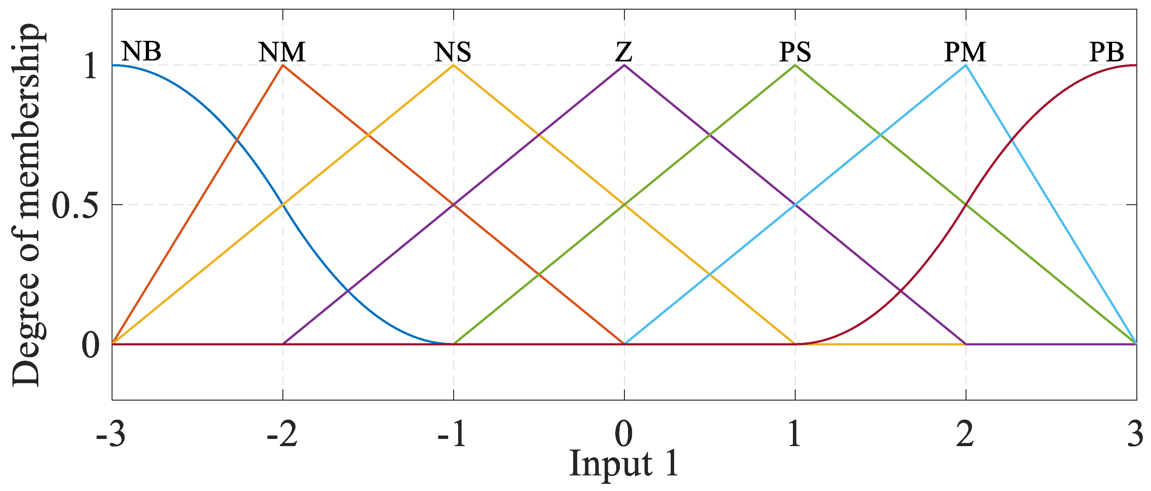
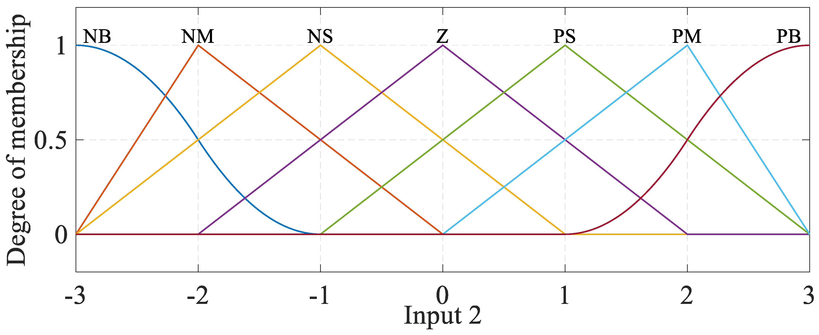
This study proposes a fuzzy controller to track the obtained generator speed. For this purpose, the generator angular speed and wind turbine actuator sensors are considered as the FLC inputs. Each input has a series of membership functions, fuzzy numbers, and linguistic variables. Figure 5 illustrates the input of the generator speed sensor. Also, Figure 6 shows the input of the wind turbine actuator sensor in the fuzzy controller. The rule base of the FLC is usually obtained from expert knowledge or heuristics, and it contains a set of 49 fuzzy rules expressed as a set of IF-THEN rules, as follows [30]:

R(i): If x₁ is F₁ and x₂ is F₂, THEN y is R(i);

i = 1, 2, 3, …, 49

where x₁, x₂, and y are input1 variable, input2 variable, and control variable, respectively. F₁ and F₂ illustrate the fuzzy sets of input1 and input2, and R(i) shows the fuzzy set of the control variable. The control rules are designed to assign a fuzzy set of the control input y for each combination of fuzzy sets of x₁ and x₂. Table 1 shows the rules for the FLC.

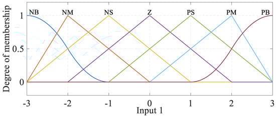
Figure 5. Membership functions for input₁ (the generator speed sensor).

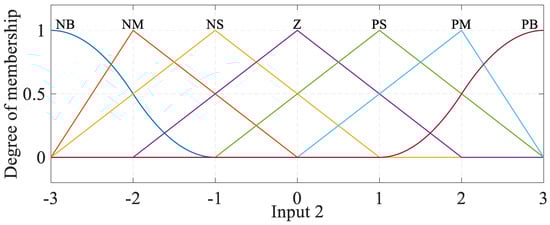
Figure 6. Membership functions for input₂ (wind turbine actuator sensor).

Table 1. Rule base for the FLC.

y		x1
		NB	NM	NS	Z	PS	PM	PB
x2	NB	NB	NB	NM	NM	NS	NS	Z
	NM	NB	NM	NM	NS	NS	Z	PS
	NS	NM	NM	NS	NS	Z	PS	PS
	Z	NM	NS	NS	Z	PS	PS	PM
	PS	NS	NS	Z	PS	PS	PM	PM
	PM	NS	Z	PS	PS	PM	PM	PB
	PB	Z	PS	PS	PM	PM	PB	PB

where NB, NM, NS, ZR, PS, PM, PB, B, and S are fuzzy set labels defined in Table 2.

Table 2. Definition of the fuzzy set labels.

Fuzzy Sets Labels	Fuzzy Sets
NB	Negative Big
NM	Negative Medium
NS	Negative Small
ZR	Zero
PS	Positive Small
PM	Positive Medium
PB	Positive Big

Figure 5 shows the input of the generator speed sensor of the wind turbine in the fuzzy controller. Table 3 illustrates the membership functions, fuzzy set labels, and fuzzy numbers of each variable.

Table 3. Membership function, fuzzy set labels, and fuzzy numbers representation for Figure 5.

Membership Function Type	Fuzzy Sets Labels	Fuzzy Numbers
zmf	NB	[−3k1, −k1]
trimf	NM	[−3k1, −2k1, 0]
trimf	NS	[−3k1, −k1, k1]
trimf	Z	[−2k1, 0, 2k1]
trimf	PS	[−k1, k1, 3k1]
trimf	PM	[0, 2k1, 3k1]
zmf	PB	[k1, 3k1]

Figure 6 shows the input of the wind turbine actuator sensor in the fuzzy controller, and Table 4. represents membership functions, fuzzy set labels, and fuzzy numbers of each variable.

Table 4. Membership function, fuzzy set labels, and fuzzy numbers representation for Figure 6.

Membership Function Type	Linguistic Variables	Fuzzy Numbers
zmf	NB	[−3k1, −k1]
trimf	NM	[−3k1, −2k1, 0]
trimf	NS	[−3k1, −k1, k1]
trimf	Z	[−2k1, 0, 2k1]
trimf	PS	[−k1, k1, 3k1]
trimf	PM	[0, 2k1, 3k1]
zmf	PB	[k1, 3k1]

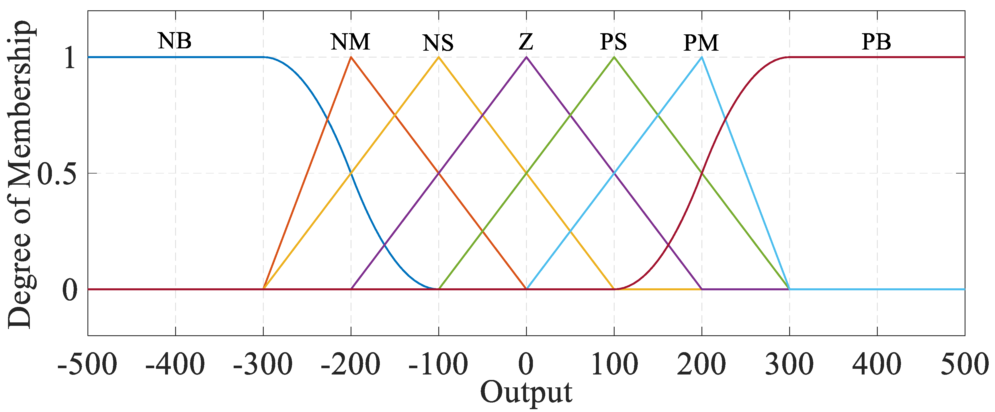
Figure 7 shows the FLC output membership functions, and Table 5. represents membership functions, fuzzy set labels, and fuzzy numbers for each variable.

Figure 7. Membership functions for output.

Table 5. Membership function, fuzzy set labels, and fuzzy numbers representation for Figure 7.

Membership Function Type	Linguistic Variables	Fuzzy Numbers
zmf	NB	[−3k3, −k3]
trimf	NM	[−3k3, −2k3, 0]
trimf	NS	[−3k3, −k3, k3]
trimf	Z	[−2k3, 0, 2k3]
trimf	PS	[−k3, k3, 3k3]
trimf	PM	[0, 2k3, 3k3]
zmf	PB	[k3, 3k3]

3. Results

In order to verify the proposed parameter estimation and MPPT implementation, the simulation was performed in a Matlab/Simulink environment. Table 6 lists the parameters of the proposed system. The simulation time frame is supposed to be 20 s, which involves the wind turbine FLC and generator speed determination with EKF. The simulated PMSG-based wind turbine and its control systems for SSC and GSC are shown schematically as Figure 8.

Table 6. Parameters of the proposed system.

Parameters	Value
Turbine Nominal Power	900 kW
Nominal Voltage	20 kV
Nominal Frequency	60 Hz
Number of Pole Pairs (P)	4
Stator Resistance (Rs)	25 mΩ
Stator Inductance (Ls)	5 mH
DC-link Capacitance (C)	2.5 mf
GSC Resistance (Rg)	15 m Ω
GSC Inductance (Lg)	0.2 mH
Switching Frequency	1590 Hz
Wind Speed	5 to 16 m/s
SSC Controller (PI1)	$\frac{5\mathrm{s}+25}{\mathrm{s}}$
GSC Current Controller (PI2)	$\frac{0.2\mathrm{s}+15}{\mathrm{s}}$
GSC Voltage Controller (PI3)	$\frac{0.62\mathrm{s}+0.01}{\mathrm{s}}$

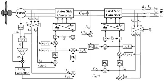
Figure 8. Proposed PMSG structure and control method.

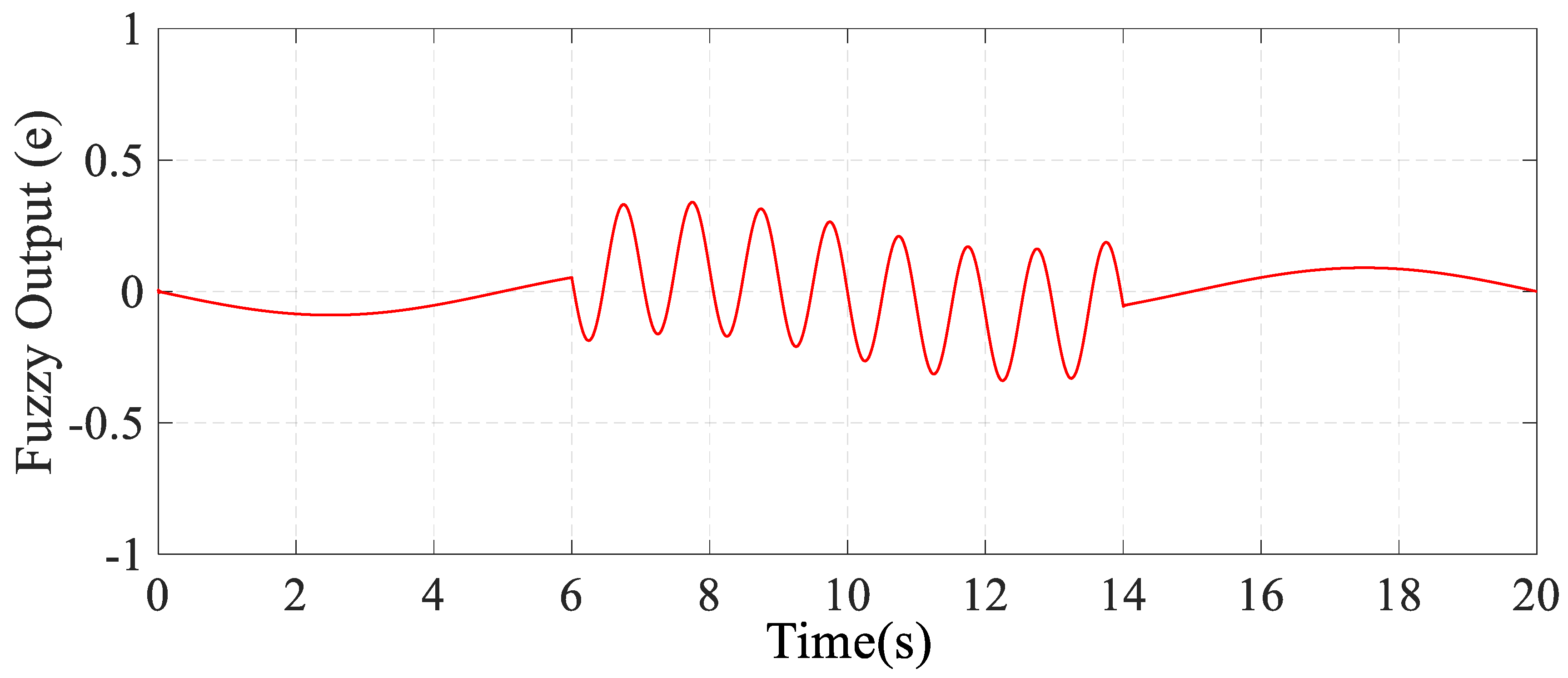
Figure 9 shows the FLC output error. A 10% oscillation in wind speed (from t = 6 s to t = 14 s) is considered to illustrate the fuzzy logic controller’s ability to track the reference speed. It can be seen that the FLC operates efficiently, even during the wind speed oscillation period. The weights in the EKF are adjusted by the defined error ($e$). The use of the fuzzy controller is aimed at resetting $1-\left(x_0+\mathrm{\Delta }x\right)$ to zero.

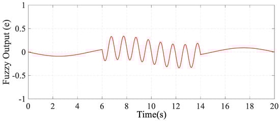
Figure 9. FLC output error.

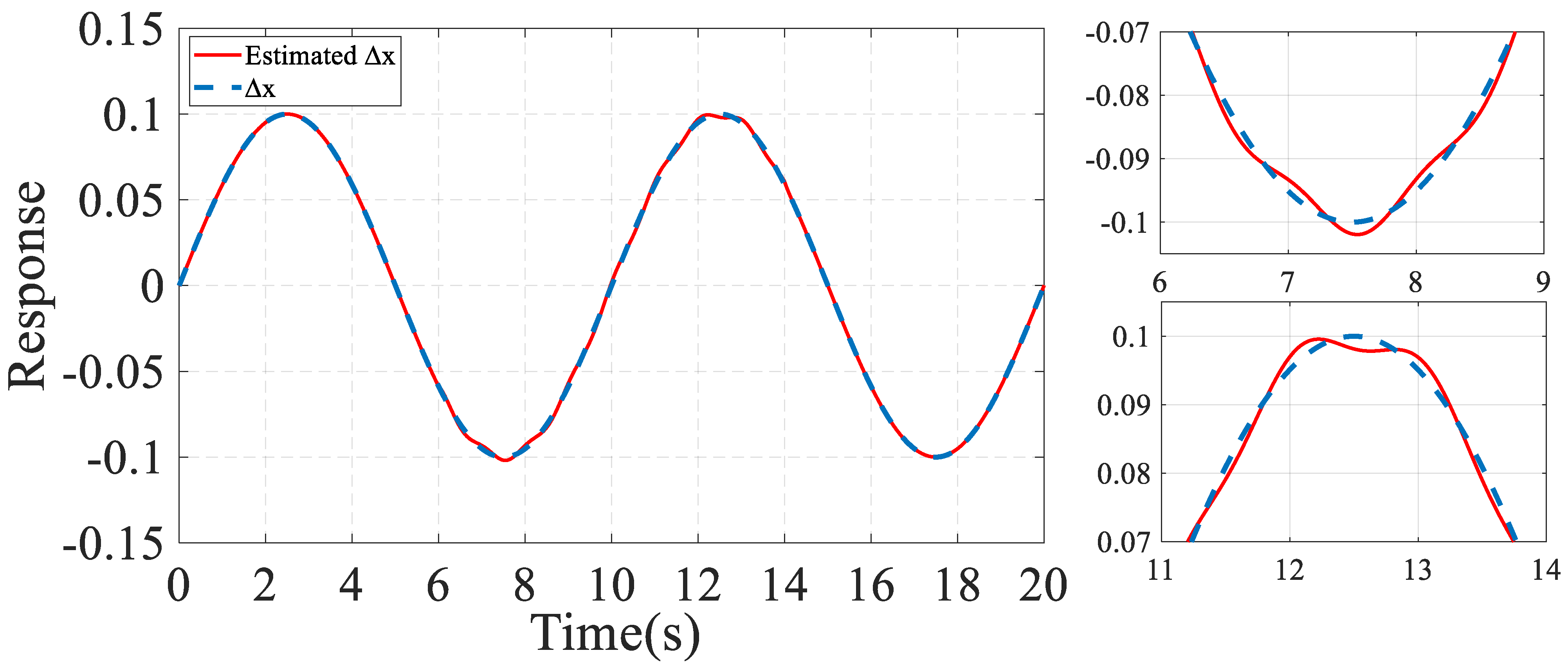
Figure 10 shows a comparison between $\mathrm{\Delta }x$ and, $\mathrm{\Delta }\widehat{x}$. It can be deduced from Figure 10 that the estimated vector of parameters is very close to its actual value. Also, the similarity between the EKF estimation and actual values during the oscillation period does not decrease significantly.

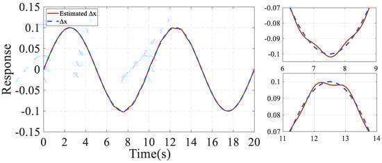
Figure 10. Comparison between the estimated $\mathrm{\Delta }\widehat{x}$ and $\mathrm{\Delta }x$.

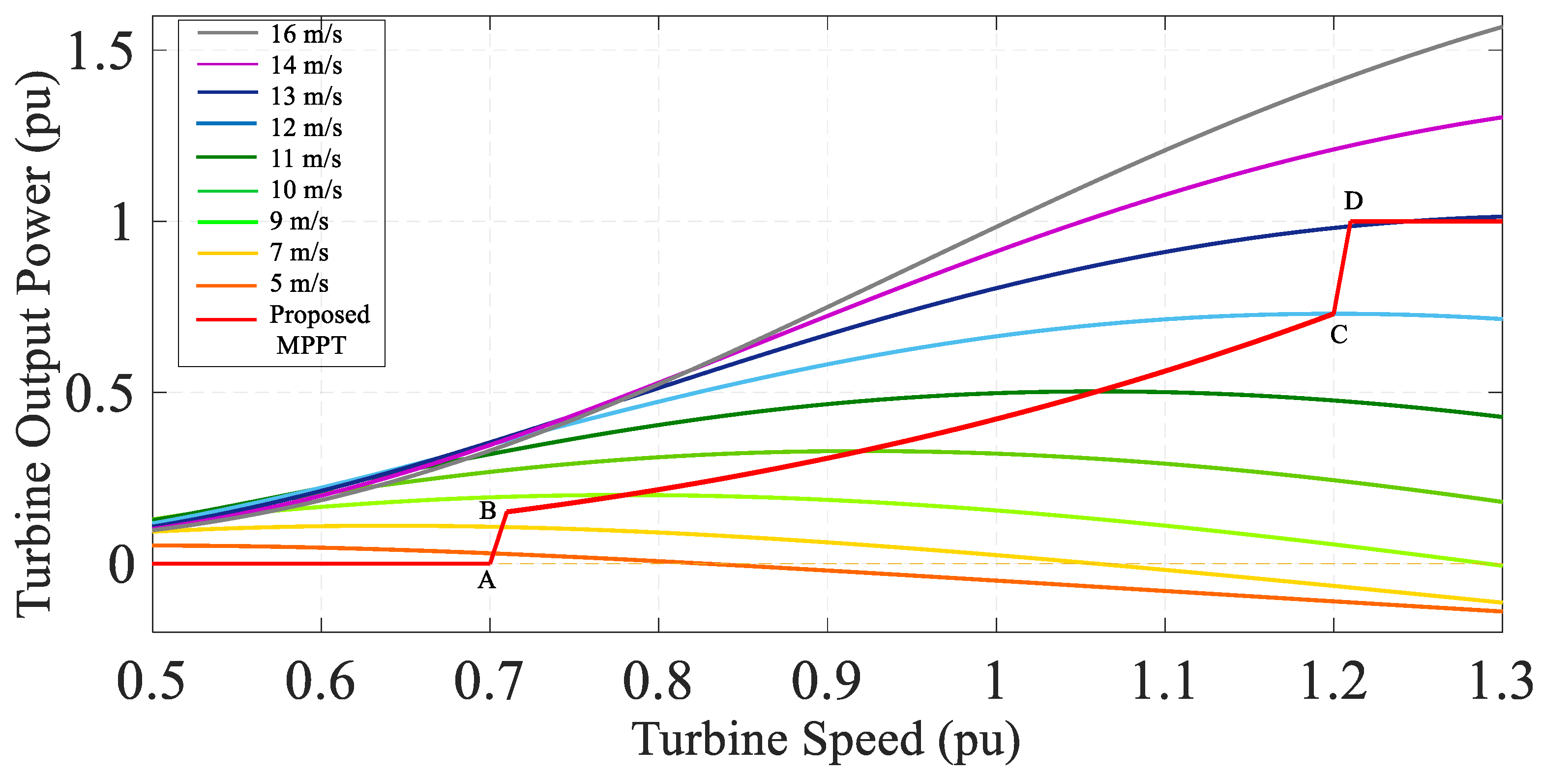
Figure 11 aims to illustrate the ability of the proposed method to track the maximum output power of the PMSG through different wind speeds. In other words, Figure 11 shows the impact of the accurate estimation of the uncertain parameters. The maximum available error is 2.049, the mean is 0.54, and the system error after applying the proposed approach is 0.708. This means a 1.341-unit accuracy improvement and efficiency of the proposed method in tracking the acerate maximum power points.

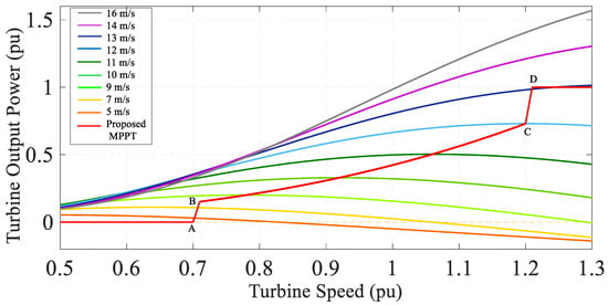
Figure 11. Proposed MPPT for different wind speeds.

4. Discussion

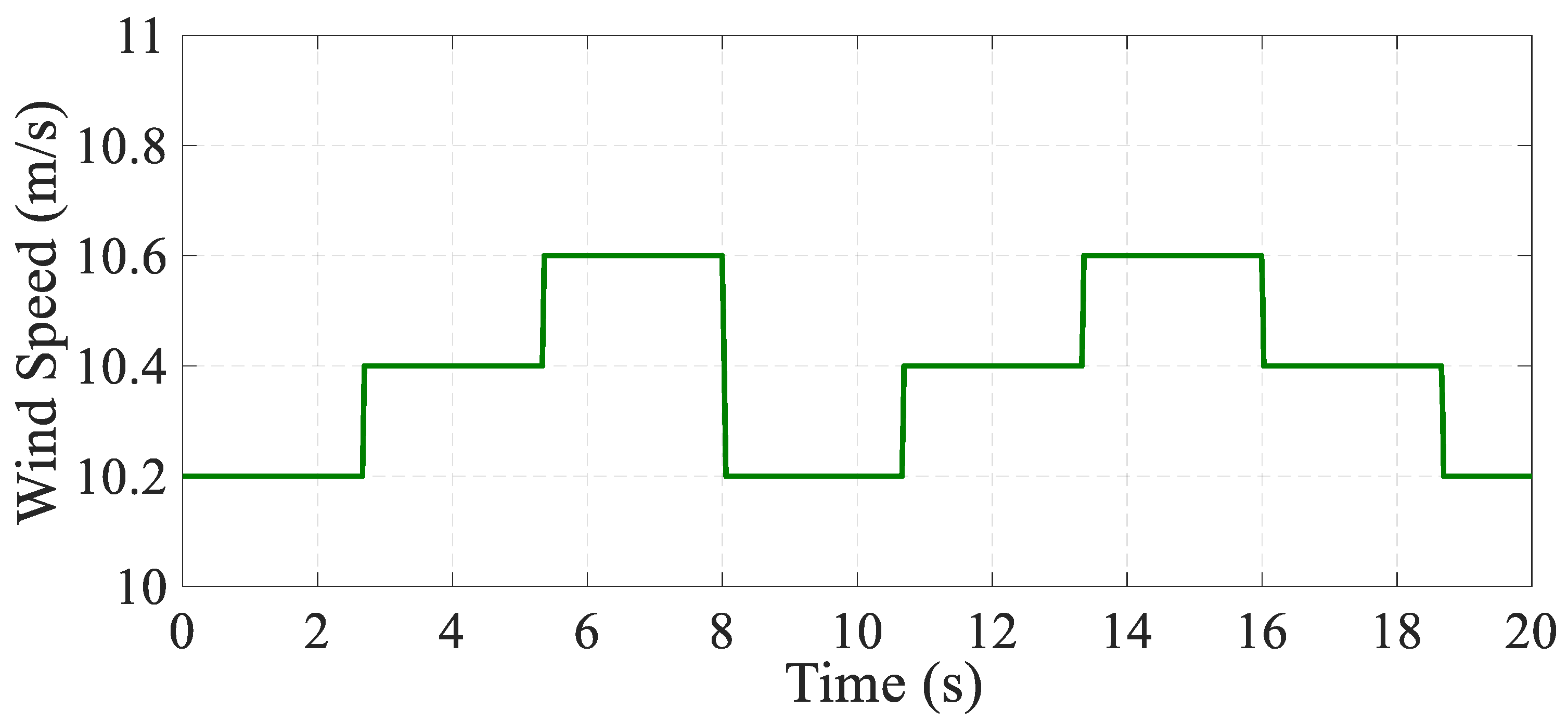
To highlight the advantages of the proposed strategy, a conventional MPPT method (using the perturb and observe method) was simulated, and the results will be compared. For this purpose, a 20-s wind speed oscillation is designed, as shown in Figure 12.

Figure 12. Wind speed scenario applied to the PMSG system.

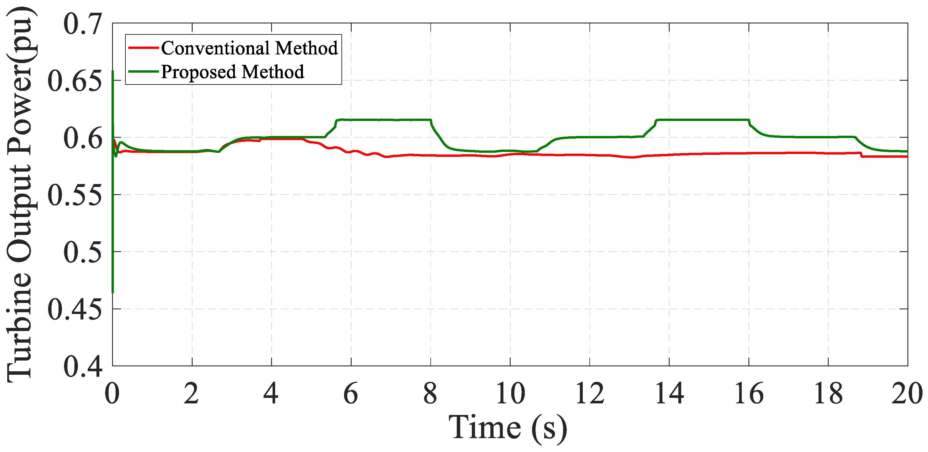
Figure 13 illustrates the generator speed comparison between the proposed strategy and the conventional model. As mentioned earlier, the accuracy of the proposed strategy during the wind speed oscillations is significantly greater than that of the conventional model. This accuracy improvement leads to utilizing more output power than the conventional strategy, as shown in Figure 14.

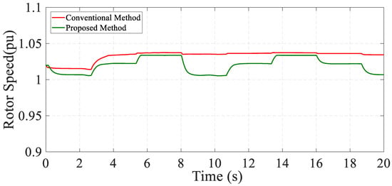
Figure 13. Comparison between the generator speed in the proposed system and the conventional method.

Figure 14. Comparison between the output power in the proposed system and the conventional method.

5. Conclusions

This paper has introduced a strategy for improving the MPPT implementation accuracy of PMSG-based wind turbines using EKF and FLC. The presented method improves the estimation of generator speed reference and can extract the optimum generator power, especially during the small oscillations of the wind speed. None of the papers that have tried to improve the estimation accuracy [22,23,24] and other papers presented so far have addressed this idea on the PMSG wind turbine by estimating unpredictable parameters, which can significantly improve the accuracy of MPPT implementation. For this purpose, the unpredictable parameters were first identified, and then the generator speed was determined by the uncertainty estimation of these parameters. Finally, the FLC controlled the generator angular speed to extract the optimum output power of the generator through the modulation indexes. The obtained results validate the proposed strategy’s effectiveness compared to the traditional one (P&O), in which a 1.341-unit accuracy improvement has been shown in estimating the optimum speed and tracking the maximum output power over different wind speeds. Moreover, the superiority of the introduced method over the conventional strategy at the same switching between different wind speeds was depicted.

References

- Yamakawa, C.K.; Qin, F.; Mussatto, S.I. Advances and opportunities in biomass conversion technologies and biorefineries for the development of a bio-based economy. Biomass Bioenergy 2018, 119, 54–60. [Google Scholar] [CrossRef]
- Honarbari, S.; Bidgoli, M.A. Designing a Quasi-Z-Source Inverter with Energy Storage to Improve Grid Power Quality. IETE J. Res. 2020, 1–9. [Google Scholar] [CrossRef]
- Zaboli, M.; Ajarostaghi, S.S.M.; Saedodin, S.; Pour, M.S. Thermal Performance Enhancement Using Absorber Tube with Inner Helical Axial Fins in a Parabolic Trough Solar Collector. Appl. Sci. 2021, 11, 7423. [Google Scholar] [CrossRef]
- Olfian, H.; Ajarostaghi, S.S.M.; Ebrahimnataj, M. Development on evacuated tube solar collectors: A review of the last decade results of using nanofluids. Sol. Energy 2020, 211, 265–282. [Google Scholar] [CrossRef]
- Roy, S.; Saha, U.K. Review on the numerical investigations into the design and development of Savonius wind rotors. Renew. Sustain. Energy Rev. 2013, 24, 73–83. [Google Scholar] [CrossRef]
- Javadi, H.; Urchueguia, J.F.; Ajarostaghi, S.S.M.; Badenes, B. Numerical Study on the Thermal Performance of a Single U-Tube Borehole Heat Exchanger Using Nano-Enhanced Phase Change Materials. Energies 2020, 13, 5156. [Google Scholar] [CrossRef]
- Javadi, H.; Urchueguia, J.; Ajarostaghi, S.M.; Badenes, B. Impact of Employing Hybrid Nanofluids as Heat Carrier Fluid on the Thermal Performance of a Borehole Heat Exchanger. Energies 2021, 14, 2892. [Google Scholar] [CrossRef]
- Alamian, R.; Shafaghat, R.; Amiri, H.A.; Shadloo, M.S. Experimental assessment of a 100 W prototype horizontal axis tidal turbine by towing tank tests. Renew. Energy 2020, 155, 172–180. [Google Scholar] [CrossRef]
- Bilandzija, N.; Voca, N.; Jelcic, B.; Jurisic, V.; Matin, A.; Grubor, M.; Kricka, T. Evaluation of Croatian agricultural solid biomass energy potential. Renew. Sustain. Energy Rev. 2018, 93, 225–230. [Google Scholar] [CrossRef]
- Ezoji, H.; Shafaghat, R.; Jahanian, O. Numerical simulation of dimethyl ether/natural gas blend fuel HCCI combustion to investigate the effects of operational parameters on combustion and emissions. J. Therm. Anal. Calorim. 2018, 135, 1775–1785. [Google Scholar] [CrossRef]
- Ezoji, H.; Ajarostaghi, S.S.M. Thermodynamic-CFD analysis of waste heat recovery from homogeneous charge compression ignition (HCCI) engine by Recuperative organic Rankine Cycle (RORC): Effect of operational parameters. Energy 2020, 205, 117989. [Google Scholar] [CrossRef]
- Wang, C.; Wang, L.; Shi, L.; Ni, Y. A Survey on Wind Power Technologies in Power Systems. In Proceedings of the 2007 IEEE Power Engineering Society General Meeting, Tampa, FL, USA, 24–28 June 2007; pp. 1–6. [Google Scholar]
- Lan, J.; Patton, R.J.; Zhu, X. Fault-tolerant wind turbine pitch control using adaptive sliding mode estimation. Renew. Energy 2018, 116, 219–231. [Google Scholar] [CrossRef]
- Gao, R.; Gao, Z. Pitch control for wind turbine systems using optimization, estimation and compensation. Renew. Energy 2016, 91, 501–515. [Google Scholar] [CrossRef]
- Wang, C.-N.; Lin, W.-C.; Le, X.-K. Modelling of a PMSG Wind Turbine with Autonomous Control. Math. Probl. Eng. 2014, 2014, 85617. [Google Scholar] [CrossRef]
- Geng, H.; Yang, G. Output Power Control for Variable-Speed Variable-Pitch Wind Generation Systems. IEEE Trans. Energy Convers. 2010, 25, 494–503. [Google Scholar] [CrossRef]
- Bianchi, F.; Mantz, R.; Christiansen, C. Gain scheduling control of variable-speed wind energy conversion systems using quasi-LPV models. Control Eng. Pract. 2005, 13, 247–255. [Google Scholar] [CrossRef]
- Stol, K.A.; Balas, M.J. Periodic Disturbance Accommodating Control for Blade Load Mitigation in Wind Turbines. J. Sol. Energy Eng. 2003, 125, 379–385. [Google Scholar] [CrossRef]
- Mohamed, A.Z.; Eskander, M.N.; Ghali, F.A. Fuzzy logic control based maximum power tracking of a wind energy system. Renew. Energy 2001, 23, 235–245. [Google Scholar] [CrossRef]
- Shi, F.; Patton, R. An active fault tolerant control approach to an offshore wind turbine model. Renew. Energy 2015, 75, 788–798. [Google Scholar] [CrossRef]
- Najafi-Shad, S.; Barakati, S.M.; Yazdani, A. An effective hybrid wind-photovoltaic system including battery energy storage with reducing control loops and omitting PV converter. J. Energy Storage 2020, 27, 101088. [Google Scholar] [CrossRef]
- Gliga, L.I.; Chafouk, H.; Popescu, D.; Lupu, C. Diagnosis of a Permanent Magnet Synchronous Generator using the Extended Kalman Filter and the Fast Fourier Transform. In Proceedings of the 2018 7th International Conference on Systems and Control (ICSC), Valencia, Spain, 24–26 October 2018; pp. 65–70. [Google Scholar]
- Afrasiabi, S.; Afrasiabi, M.; Rastegar, M.; Mohammadi, M.; Parang, B.; Ferdowsi, F. Ensemble Kalman Filter based Dynamic State Estimation of PMSG-based Wind Turbine. In Proceedings of the 2019 IEEE Texas Power and Energy Conference (TPEC), College Station, TX, USA, 7–8 February 2019; pp. 1–4. [Google Scholar]
- Zhang, Z.; Wang, F.; Si, G.; Kennel, R. Predictive encoderless control of back-to-back converter PMSG wind turbine systems with Extended Kalman Filter. In Proceedings of the 2016 IEEE 2nd Annual Southern Power Electronics Conference (SPEC), Auckland, New Zealand, 5–8 December 2016; pp. 1–6. [Google Scholar]
- Zerdali, E.; Yildiz, R.; Inan, R.; Demir, R.; Barut, M. Improved speed and load torque estimations with adaptive fading extended Kalman filter. Int. Trans. Electr. Energy Syst. 2021, 31, 12684. [Google Scholar] [CrossRef]
- Bagheri, A.; Ojaghi, M.; Bagheri, A. Air-gap eccentricity fault diagnosis and estimation in induction motors using unscented Kalman filter. Int. Trans. Electr. Energy Syst. 2020, 30, e12450. [Google Scholar] [CrossRef]
- Ortatepe, Z.; Karaarslan, A. Robust predictive sensorless control method for doubly fed induction generator controlled by matrix converter. Int. Trans. Electr. Energy Syst. 2020, 30, 12650. [Google Scholar] [CrossRef]
- Wu, Y.-T.; Liao, T.-L.; Chen, C.-K.; Lin, C.Y.; Chen, P.-W. Power output efficiency in large wind farms with different hub heights and configurations. Renew. Energy 2019, 132, 941–949. [Google Scholar] [CrossRef]
- Ribrant, J.; Bertling, L. Survey of failures in wind power systems with focus on Swedish wind power plants during 1997–2005. In Proceedings of the 2007 IEEE Power Engineering Society General Meeting, Tampa, FL, USA, 24–28 June 2007; pp. 1–8. [Google Scholar]
- Odgaard, P.F.; Stoustrup, J.; Kinnaert, M. Fault-Tolerant Control of Wind Turbines: A Benchmark Model. IEEE Trans. Control Syst. Technol. 2013, 21, 1168–1182. [Google Scholar] [CrossRef] [Green Version]
- Shariatpanah, H.; Fadaeinedjad, R.; Rashidinejad, M. A New Model for PMSG-Based Wind Turbine with Yaw Control. IEEE Trans. Energy Convers. 2013, 28, 929–937. [Google Scholar] [CrossRef]
- Rosyadi, M.; Muyeen, S.M.; Takahashi, R.; Tamura, J. A Design Fuzzy Logic Controller for a Permanent Magnet Wind Generator to Enhance the Dynamic Stability of Wind Farms. Appl. Sci. 2012, 2, 780–800. [Google Scholar] [CrossRef] [Green Version]
- Mehrzad, D.; Luque, J.; Cuenca, M.C. Vector Control of PMSG for Grid-Connected Wind Turbine Applications. Master’s Thesis, Institute of Energy Technology, Alborg University, Aalborg, Denmark, 2009. [Google Scholar]
- Gao, D.W. Energy Storage for Sustainable Microgrid; Academic Press: Cambridge, MA, USA, 2015. [Google Scholar]
- Wan, E.A.; van der Merwe, R.; Nelson, A.T. Advances in Neural Information Processing Systems 12, Ch. Dual Estimation and the Unscented Transformation; MIT Press: Cambridge, MA, USA, 2000; pp. 666–672. [Google Scholar]
Publisher’s Note: MDPI stays neutral with regard to jurisdictional claims in published maps and institutional affiliations. |
© 2021 by the authors. Licensee MDPI, Basel, Switzerland. This article is an open access article distributed under the terms and conditions of the Creative Commons Attribution (CC BY) license (https://creativecommons.org/licenses/by/4.0/).