Abstract
This paper presents a novel approach for improving the safety of vehicles equipped with Adaptive Cruise Control (ACC) by making use of Machine Learning (ML) and physical knowledge. More exactly, we train a Soft Actor-Critic (SAC) Reinforcement Learning (RL) algorithm that makes use of physical knowledge such as the jam-avoiding distance in order to automatically adjust the ideal longitudinal distance between the ego- and leading-vehicle, resulting in a safer solution. In our use case, the experimental results indicate that the physics-guided (PG) RL approach is better at avoiding collisions at any selected deceleration level and any fleet size when compared to a pure RL approach, proving that a physics-informed ML approach is more reliable when developing safe and efficient Artificial Intelligence (AI) components in autonomous vehicles (AVs).
1. Introduction
According to a recent study, [1], around 94% of road accidents are happening due to human errors. For this reason, considerable efforts are made by the scientific research institutions and the automotive industries in order to reach autonomous cars that are safer than human drivers [2]. These efforts are driven also by the fact that AVs are becoming influential on the social and economic development of our society [3]. Nevertheless, because usually, the AI models used in AVs are dependent on huge amounts of data and labeling efforts, which are mostly expensive and hard to obtain, this can result in so-called “black box” AI models which are limited not only due to the size of the dataset they were trained on but also due to imperfect labeling. This is a very crucial problem regarding safety because the resulting AI models which are agnostic to real physical relations and principles found in the real world, being unable to generalize well to unseen scenarios [4]. This is especially the case for accidents as the frequency of critical situations is very low, and, thus, the number of such situations in datasets collected from real-world recordings tends to be low as well.
Thus, there is a need for a new kind of AI models that are more efficient regarding safety, interpretability, and explainability, with a promising viable solution in this direction being represented by the use of so-called Informed ML [5] approaches where AI models can be improved by using additional prior knowledge into their learning process. Recently, this approach is proving to be successful in many fields and applications such as lake temperature modeling [4], MRI reconstruction [6], real-time irrigation management [7], structural health monitoring [8], fusion plasmas [9], fluid dynamics [10] and machining tool wear prediction [11]. However, regarding autonomous driving, this approach was not fully explored, with recent research projects such as KI Wissen [12] funded by the German Federal Ministry for Economic Affairs and Energy being one of of the first, if not, the first one that tries to bring knowledge integration into Automotive AI in order to increase their safety.
With regard to autonomous driving, one of many safety-critical components is considered to be the ACC, mainly due to its ability to increase safety and driving comfort by automatically adjusting the speed of the ego-vehicle according to the position and speed of a leading vehicle while following it. ACCs are also known for having several advantages over human driving such as reducing the energy consumption [13] in a vehicle or improving the traffic dynamics [14], to name only a few. Despite being available in many modern vehicles, ACCs are still heavily dependent on the available sensors equipped on them. These sensors differ for each manufacturer and model, such as radar and LIDAR, which can either have a malfunction or their sensor data readings are affected by noisy and low accuracy data [15] which can lead to instability, severe conditions regarding speed, discomfort, and even risks of collisions [16]. More than that, because ACCs are typically approached as a model-based controller design based on an Intelligent Driver Model (IDM), despite performing decently on highways, they lack the ability to adapt to environments or driving preferences, and thus, an RL-based ACC approach is seen as more favorable towards fully autonomous cars which can be fully trusted by humans. Some of the main reasons for this are the advantages of an RL-based ACC approach such as that it does not require a dataset and that training can be realized irrespective of the environment [17].
Considering these aspects, in this paper, we show, to the best of our knowledge, for the first time in literature, a PG RL approach, which is able to increase the safety of vehicles equipped with ACC by a large margin for any deceleration level and at any fleet size when compared to a pure RL approach, also in the case when the input data is perturbed. Despite the fact that platooning scenarios, even the ones using RL, have already been considered in the literature, many works focus on the yet unrealistic scenario of communicating vehicles so that each vehicle in the queue immediately receives non-perturbed information about the intended actions of all other vehicles, as seen in the work presented by the authors in [18], or which perform joint optimization as seen in the work by the authors in [19]). Similarly, the work in [20] restricts the communication between the individual vehicles but they consider platooning scenarios that differ from ours by using other control schemes (e.g., averages of four controllers) as well as by the goal of focussing on the lead vehicle of a platoon. The novelty of our approach presented in this paper is the combination of RL with deep state abstractions, reward shaping w.r.t. a safety requirement (i.e., jam-avoiding distance), perturbed inputs as well as individual behavior in an AVs platoon regarding car-following scenarios. By using the proposed PG RL approach for ACC, we demonstrate that it is possible to improve an AI model’s performance (less collisions and more equidistant travel) only by using physical knowledge as part of a pre-processed input, without the need of extra information.
The paper is organized as follows. In Section 2, we present the related work regarding different implementations of ACCs using physics or using RL. Section 3 details the proposed PG RL solution for increasing the safety of ACCs. Section 4 presents the simulation details of the car-following scenario implementation. In Section 5, we present the experimental setup and results. Finally, in Section 6, we present the conclusions and future work of this paper.
2. Related Work
Recently, the advancement of AVs technology has resulted in unique concepts and methods that allow the successful deployment of vehicles capable to drive in different levels of autonomy. However, different authors used different approaches to target safe self-driving control speed and learning navigation. In addition, there are several works that propose solutions regarding safer ACCs either using only physical knowledge or by using ML methods such as RL [21,22].
In the field of transportation engineering, the work in [23] serves as an introduction and analysis of the theoretically successful AI frameworks and techniques for AVs control in the age of mixed automation. They conclude that multi-agent RL algorithms are being preferred for long-term success in multi-AVs. The authors in [24] introduce a cooperative ACC method that makes use of an ACC controller created using the concept of RL in order to manage traffic efficiency and safety, showing impressive results in their experiments with a low-level controller. The work in [25] successfully implemented a method for Society of Automotive Engineers (SAE) low-cost modular AV by designing a vehicle unique in the industry, and which proves to be able to transport persons successfully. The approach in this work leads to the realistic application of behavioral replication and imitation learning algorithms in a stable context. The authors in [14] proposed a physics-based jam-avoiding ACC solution based on an IDM and proved that by using physical knowledge, the traffic congestion can be drastically improved by employing even a small number of vehicles equipped with ACCs. The authors in [13] propose an end-to-end vision-based ACC solution based on deep RL using the double deep Q-networks method, and which is able to generate a better gap regulated as well as a smoother speed trajectory when compared to a traditional radar-based ACC or human-in-the-loop simulation. Also, the authors in [17] proposed an RL-based ACC solution that is capable of mimicking human-like behavior and is able to accommodate uncertainties, requiring minimal domain knowledge when compared to traditional non-RL-based ACCs in congested traffic scenarios in a crowded highway as well as countryside roads. The work in [26] evaluates the safety impact of ACCs in traffic oscillations on freeways also by using a modified version of IDM in order to simulate the car-following movements using Matlab2014b software, concluding that an ACC system can significantly improve safety only when parameter settings such as larger time gaps, smaller time delays, and larger maximum deceleration rates are maintained. Physical and world knowledge was used also in other deep learning models such as regarding the off-road loss in [27] and models that respect dynamic constraints [28], both of these approaches being combined in the work presented in [29]. In addition, the authors in [30] add a kinematic layer to the model which produces kinematically conform trajectory points that serve as additional training points for prediction. World knowledge, in terms of social rules, has been integrated into deep learning models in [31] where residuals are added to knowledge-driven trajectories in order to realistically reflect pedestrian behavior, and in [32] where social interaction is invoked in order to make collision-free trajectory predictions for pedestrians. A similar work is presented also in [33], where interaction-aware trajectory predictions for vehicles are computed. Concerning the violation of traffic rules, the work in [34] uses a penalty term for adversarial agents, with the work in [35] also adding a collision reward term as well as a penalty for unrealistic scenarios. Regarding safety distance, this has been considered by the authors in [36] who added a safety distance violation penalty and a collision penalty, among others, to a hierarchical RL model, by the authors in [37], who consider a fixed safety distance in overtaking maneuvers, and also by the authors in [38], where a distance reward is invoked in car-following maneuvers.
The works mentioned in this chapter highlight the importance of safety in ACCs in the literature, indicating that by using either physics or ML-based solutions such as RL, considerably better results can be obtained. However, to the best of our knowledge, there is no work in literature that combines both physics and deep RL in order to increase the safety of ACCs. For this reason, in this paper, we combine the two approaches of physics knowledge as well that of RL into a stand-alone PG RL solution, providing a basis for future researchers to build upon.
3. Physics-Guided Reinforcement Learning for Adaptive Cruise Control
In this section, we describe the proposed approach that combines the physical knowledge in the form of jam-avoiding distance together with the SAC RL algorithm [39] in order to increase the safety of ACCs. First, we briefly introduce the SAC algorithm, followed by the physical model used, and finally, we also show their merging approach and how the integration of prior knowledge is realized in this work.
3.1. Soft Actor-Critic Algorithm
In this paper, we make use of the RL framework for training our ACC model, more exactly, of the SAC RL algorithm [39]. RL refers to a collection of learning techniques that train an agent through experience. Here, the experience is collected as a simulation in the forms of states, actions, and rewards in order to find the policy that maximizes the expected cumulative reward it obtains. One of the main advantages of RL is that it does not require a specific dataset for training, the data used for its training being generated as experience in the simulation. However, many of the existent RL algorithms found in the literature have limitations during on-policy learning such as sample inefficiency as well as during off-policy learning such as hyperparameter sensitivity and increased time required for tuning them in order to achieve convergence.
SAC [39] is an off-policy state-of-the-art RL algorithm that does not have the limitations mentioned above. This is the reason we choose to use SAC in our work. Furthermore, we deal with continuous action spaces where SAC is not efficient in maximizing the reward but still in maximizing the entropy of the policy. This is important as a higher entropy encourages a higher exploration of the state space by the agent and improves the convergence [39]. In order to achieve such improvements using a random strategy over other RL algorithms that use deterministic strategy, SAC according to [39] makes use of soft Q-learning, relying on two different function approximators such as a soft Q-value function as well as a stochastic policy which are optimized alternately. The soft Q-function with describing the state at time t and the action at time t, is parametrized by . The tractable policy , containing the state-action pair, is parametrized with .
3.2. Prior Knowledge
From traffic experiences as well as from governmental traffic rules, it is known that traffic participants have to ensure a sufficient safety distance to each other, to avoid possible collisions. Besides this prior world knowledge, there is also conjunctive physical knowledge on how the distance between an agent and a leading vehicle can be controlled. An example regarding this aspect is given by the authors in [14] who extend an existing IDM-Model in order to realize an ACC lane following controller with model parameters in Table 1. Based on that desired parameters such as velocity, acceleration constraints, and minimum distance for jam-avoiding, the authors present the desired acceleration for a jam-free lane as seen in Equation (1) [14].

Table 1.
Static model parameters used in the proposed approach for increasing the safety of ACC [14].
Here, s is the distance to the leading vehicle and describes the minimum jam-avoiding distance depending on the current agent velocity v and the velocity difference to the leading vehicle.
Together with a static minimum distance for low velocities, the save time headway T and desired deceleration and maximum acceleration b and respectively, results to the Equation (2) [14]:
Considering the goal of this paper, we make use of Equation (2) when integrating prior knowledge into the SAC RL algorithm.
3.3. Integration of Prior Knowledge
The main goal of the integration is to help the autonomous agent learn the correct control actions that result in reasonable trajectories. Regarding this aspect, one can distinguish essentially between supervised and non-supervised algorithms for such problems. Supervised approaches like constrained control algorithms [40] optimize a particular objective function constrained to some hard constraints which formalize safety requirements. By solving the respective constrained optimization problem, the ego-trajectory is guaranteed to satisfy the safety constraints. A major drawback of these supervised strategies is that they require target/reference trajectory points and velocities, to name only a few, which are usually difficult to obtain [41]. In contrast, RL cannot cope with hard constraints but poses them as soft constraints (where their severity depends on the regularization parameter ) onto the objective function. The main advantage is, however, that RL does not require any data but generates the data during training where it learns which trajectories and therefore, which control actions are reasonable in which situation by receiving reward feedback, so actions that severely violate the constraints lead to very low rewards. In our work, we design the regularization term of the reward function, i.e., the soft constraint, so that it represents the safety constraint in order to keep the optimal jam-avoiding distance, encouraging the agent to respect this safety constraint.
Following, we present our merging approach between the SAC architecture and the physical knowledge. As can be seen in Figure 1, a typical regular RL approach for ACC (black arrows) considers information about relative velocity and front vehicle distance based on radar systems. In addition, the current velocity is taken into account by the actor networks. According to this raw data by the sensors, the normal RL approach is deciding about the next acceleration steps. However, regarding the overall ACC goal of driving in perfect target separation as often as possible, the proposed PG RL approach is taking an important relation, namely the jam-avoiding distance (red arrows), between the raw data into account. By considering the jam-avoiding distance with the sensor data and the model parameters seen in Table 1, the actor-network is better prepared than the normal RL approach on finding an optimal policy for the ACC.
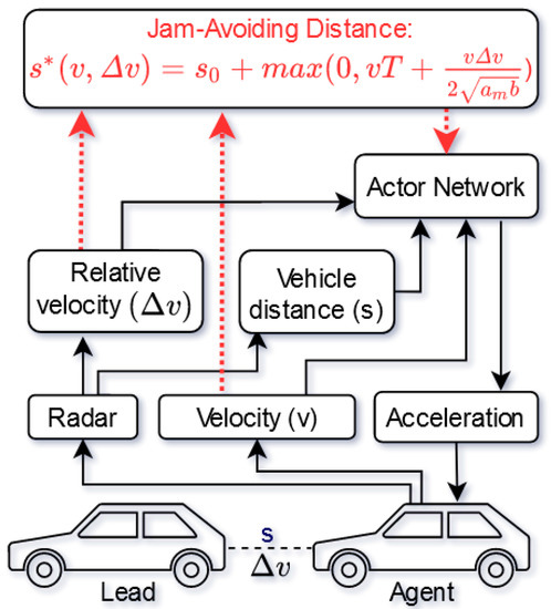
Figure 1.
Proposed PG RL approach for increasing the safety of ACC by integrating prior knowledge in the form of the Jam-Avoiding Distance.
A more detailed explanation for the choice of this physical knowledge is explained later in the States subsection of this paper. In addition, a comparison and evaluation between both approaches are detailed in Section 5.
4. Simulation
Regarding the ACC system, we implemented a car-following scenario. For the scenario, we consider an urban road and normal weather conditions without influencing any fraction coefficients. In the main simulation, we assume perfect perception without perturbations s.t. all required data and information are available at any time; however, afterwards, we also performed the same procedures but introducing perturbations. The basic setup consists of two vehicles, a leading vehicle and one following vehicle, which contains the acting agent calculating the acceleration of the agent vehicle. Initially, the distance between the vehicles is 20 m. Based on the adapted physical IDM [14], the static model parameters applied are the ones presented earlier in Table 1. Following the RL approach and the physical model, for each simulation step, the acceleration to be executed is determined by the actor-network by extrapolating the current state to the next partial state based on the current position and velocity. Here, the resulting velocity and position, which are the relation values for the used physical model and the environment, are determined by the Eulers method seen in Equation (3):
with the step size .
The resulting velocity of an agent is thus determined in each simulation step with Equation (4):
where is the velocity at time t and is the acceleration determined by the artificial neural network at time .
The same procedure is also used to determine the new position of an agent with Equation (5):
where is the position at time t.
4.1. Leading Agent Acceleration
The only parameter that is not directly handled by the physical model and the virtual environment is the acceleration of the leading vehicle. In order to enable a simulation also for the leading vehicle, we need an acceleration replacement, such as one of the following heuristics presented in Table A1:
- Random acceleration at each time step (randomAcc),
- Constant acceleration with random full stops (setting lead velocity with ) (randomStops9 accelerates by 90% of its capacity and randomStops10 accelerates full throttle)
- Predetermined acceleration for each time step (predAcc).
Based on the simulation performance with the test results presented in Section 4.6, the predetermined acceleration heuristic was chosen in the following manner: first, the vehicle will accelerate at 0.8 of its maximum acceleration until reaching half of its maximum speed. In this part, the agent will have to learn to accelerate but will not be able to accelerate at maximum capacity, being forced to also learn some control. Secondly, the vehicle will decelerate constantly until it stops. This will force the agent to learn to brake. Finally, it will repeat the first two steps, but accelerating at 0.9 of its maximum capacity, thus forcing the agent to accelerate at a greater capacity and then brake from a higher velocity as well.
4.2. States
The overall MDP is given by the tuple with the state space , the action space , a deterministic transition model and rewards r. A discount factor is not considered in this work. The goal is to learn a deterministic parametric policy .
Regarding the state space, the simulation is fundamentally driven by three different parameters. One parameter to consider is the separation between agents. The second parameter is the speed difference between the agent and the lead vehicle (approaching velocity). Lastly, the speed of the acting agent is observed. Here, because the Q-function is modeled as an expressive neural network in the SAC algorithm [39], for faster processing, the value domains of the parameters were normalized to the interval [0, 1].
Based on the integration of the physical model from [14] and the consequently relevant target separation , two further indicators are introduced for the simulation. First, the target separation itself is observed as a parameter. This was also normalized to the interval [0, 1]. Secondly, a Boolean was introduced, which indicates whether the current separation is smaller (0) or larger (1) than the target separation. The reason for introducing this value was to provide the agent with an additional indicator for improving the determination of the acceleration that needs to be executed. In Section 5, we will evaluate the impact of adding this physical knowledge as inputs to the agent in the learning process.
Regarding the action space, we translated the asymmetric interval ranging from the maximum negative deceleration to the maximum acceleration into the symmetric interval .
4.3. Penalization
Based on the present scenario with an ACC system, in case of a collision with the agent in front an agent is penalized with a negative reward. In this work, different magnitudes from 0 to 10 for the execution of the penalization were tested. We discovered that if the penalization for the collision of an agent is too large, in order to avoid collisions, the agent may learn not to move at all. On the other hand, if the penalization is too small, the agent may ignore this misbehavior. In order to handle the adjustment of the correct penalization magnitude, a test attempt was made to introduce another penalization for not moving. Finally, after experimenting with different magnitudes we discovered that a relatively small collision penalization of 3000 has been working the best, this penalization value being applied when the agent collides (meaning that the resulting reward will be reduced by 3000). We observed that a good but riskier policy achieves a better learning result due to the chosen reward function than the search for a possibly fundamentally new strategy due to a high collision penalization. Thus, in the case of a good but risky policy, the selected reward function is taking a collision risk more into account. More detailed information about the test results can be seen in Section 4.6.
4.4. Reward
In the course of several simulations, several different reward functions were considered. First, a target distance reward that evaluates the absolute difference between the current separation of the vehicle and the target separation was tested (named as absoluteDiff in Table A1). This metric was not useful due to the bias introduced into being closer to the lead vehicle rather than farther behind. A second reward function tested was related to velocity (named as velocity in Table A1): the faster the vehicles follow each other without collision, the better the strategy was. We observed that, when considering possible speed limits, this reward function can only slightly lead to an improvement of an already good but not optimal strategy in the search space. The last reward function examined does not contain an evaluation of a strategy but only the penalization if a collision occurs or if the agent does not move (named as None in Table A1). It is important to mention that a liveness reward that encourages the agent to move must however be designed with caution since the maximal liveness reward should be very small regarding absolute value in comparison to penalties for violating the speed limit.
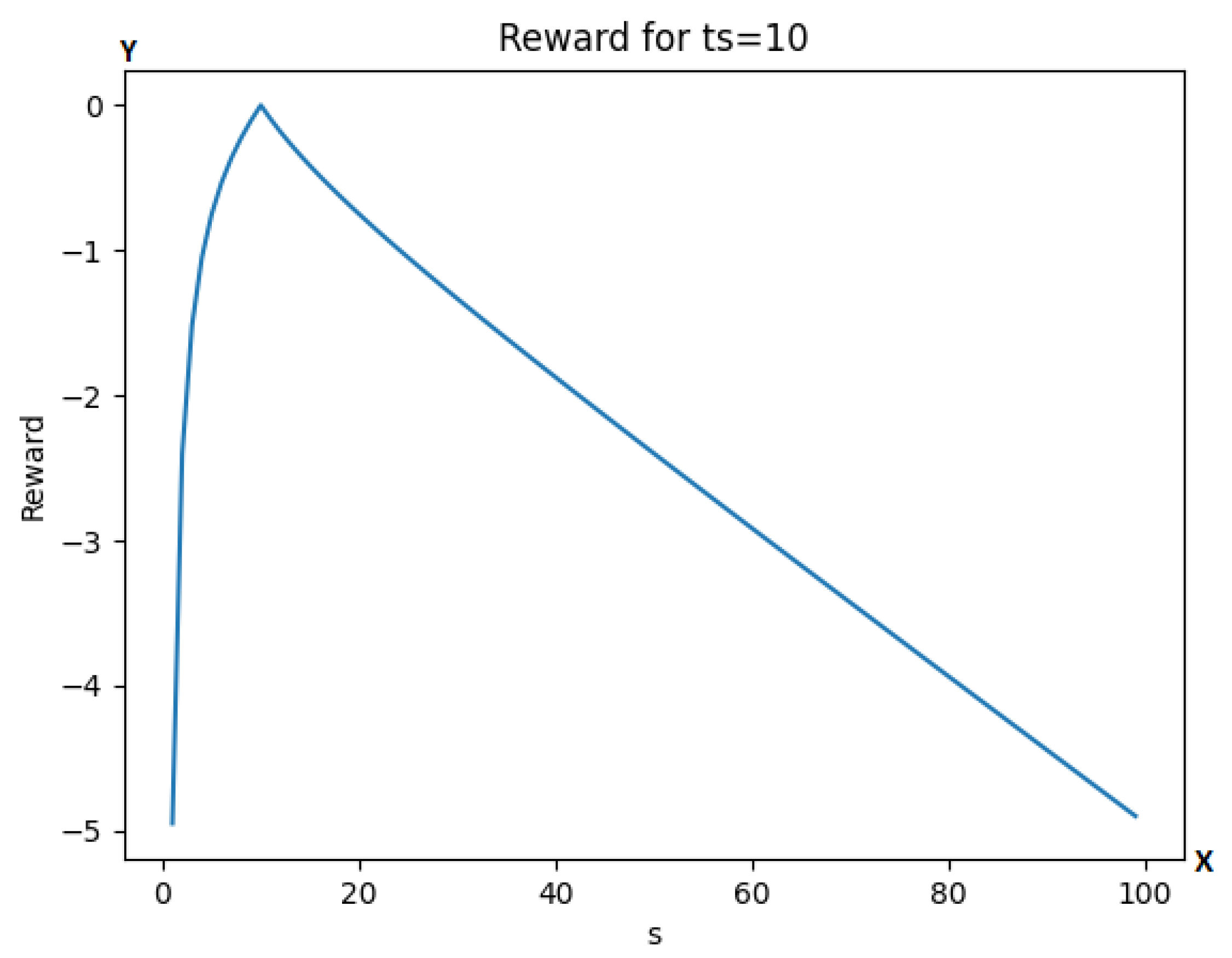
Across our simulations, the following target distance reward function (named as symmetric in Table A1) performed the best. More exactly, the reward of a performed action was then determined by Equation (6):
with being the target separation at the given speed. This reward has only one optimal point at . The reward is also symmetrical to its variables, so for example if or are considered, the reward value is the same in both cases, as can be also observed in Figure 2 with (for different values of ts the function has the same properties). More detailed information about the test results can be seen in Section 4.6.
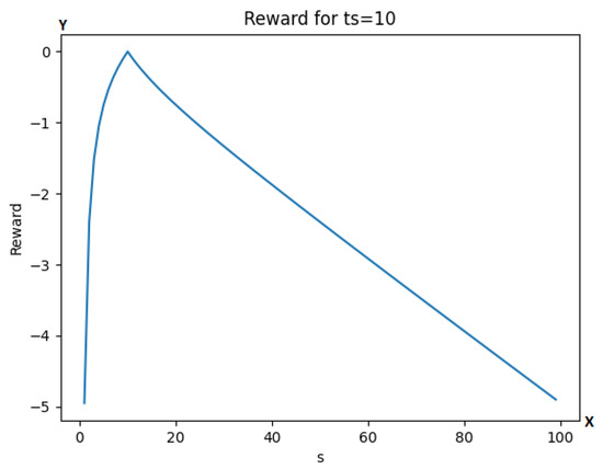
Figure 2.
Graph of the reward function for different values of s at . The y-axis is representing the reward value, while the x-axis is representing the number of simulation steps.
4.5. Termination Conditions
As termination conditions for a simulation run, we consider the goal of the system to be that of traveling as fast as possible while producing no collisions. This requires a suitable termination criterion for the simulation to be found. In our tests, we observed that the sole inclusion of collision in the termination criterion leads to the fact that the simulation does not end when the agents have found an optimal policy. We also found that, if a fixed period of time is included in the termination criterion, an acting agent can find a good policy by merely driving slowly within this fixed period. Finally, we observed that a termination after a certain number of simulation steps was more reasonable. Therefore, the chosen termination criterion for the simulation is a combination of a collision consideration and a certain number of simulation steps.
4.6. Parameter Search Test
Considering the high number of choices there are to make in the realms of reward, penalization and lead vehicle behavior, we performed trainings for each possible combination of a set of parameters. More exactly, for the lead vehicle behavior, the possibilities considered are the ones described earlier in Section 4.1 (randomAcc, randomStops9, randomStops10, and predAcc). Regarding the reward, the possibilities considered are the ones described earlier in Section 4.4 (symmetric, velocity, absoluteDiff and None). Regarding the penalization, the values considered were 0, 100, 3000 and 100,000. This gives us a total of 64 different combinations of parameters. In order to find the best set of parameters, for each of the 64 different combinations, we train the model for 1,000,000 iterations and then perform an evaluation in order to find the Headway (HW) and Time Headway (THW) criticality metrics [42] of a single agent following a lead vehicle accelerating and suddenly stopping at two different points (this is done 10 times in order to average the results) and also an evaluation involving 12 agents and a lead vehicle (behaving similarly to the previous test) in order to evaluate the final positions of the vehicles (this is also performed 10 times and averaged). At any of the 20 tests, if there is a collision, the test ends and a collision is counted before continuing to the following test. From the results of these tests, we not only want to see a low collision count but also a reasonable THW (preferably between 1 and 3 s). Here, higher THW indicates that the agent is very slow, while low THW is risky. As we can see in Table A1, row 33, the model 3000/predAcc/symmetric (meaning penalization is 3000, the lead agent performs predetermined accelerations and reward is the symmetric one) is the only model with 0 collisions while having a good THW (2.25).
We can also see that penalizations of 0 and 100 are too low and because of that the models tend to have more collisions, while a penalization of 100,000 produces little to no collisions but barely accelerates (as seen in the case of high THW values presented in Table A1). We can observe that the random accelerations for the lead vehicle produce extremely cautious agents (as seen in the high THW values presented in Table A1). The same thing can be said about random stops, even though the impact is not as drastic. Finally we can see that velocity and absoluteDiff rewards lead to a lot of collision, while no reward as expected produces really slow agents. Considering these results, we will use a penalization of 3000, a predetermined acceleration lead agent behavior, and the custom reward symmetric.
4.7. Perturbed Inputs
The main focus of our work is on the perfect scenario where the velocity, the distance to the leading vehicle, and its velocity are accurately known at every step. However, we also run all the experiments in a secondary simulation in which a perturbation is introduced in the form of a random multiplier of uniform value between 0.9 and 1.1 which is applied to each of the three mentioned variables.
4.8. Training Setup
Regarding training setup, we made use of the Ubuntu distribution of Linux, version 20.04, together with Tensorflow 2.4.1; here, we also made use of Reverb 0.2.0 framework [43] as the experience replay system for RL. Regarding training, we trained each model for 1 million iterations of the simulation, using the same architectures (except for the fact that one has more input and in turn more connections) for both neural networks composed of a single hidden layer with 500 neurons. The reason for choosing these architectures was their low-dimensional feature space.
5. Evaluation
The objective of this section is to show the advantages of adding physical knowledge to the RL model found in ACC and to prove that vehicles equipped with a PG RL-based ACC are safer. With that in mind, we will compare results in different tasks between a traditional RL model and our proposed PG RL model, in which we introduce prior knowledge, as explained in the previous section. The tasks will consist of a lead agent with a predetermined acceleration being followed by one or more agent vehicles controlled by one of our models, at a predetermined initial separation distance. For this, we will evaluate how likely each of the models is to collide, and how well the agents controlled by the models spread out.
5.1. Task 1
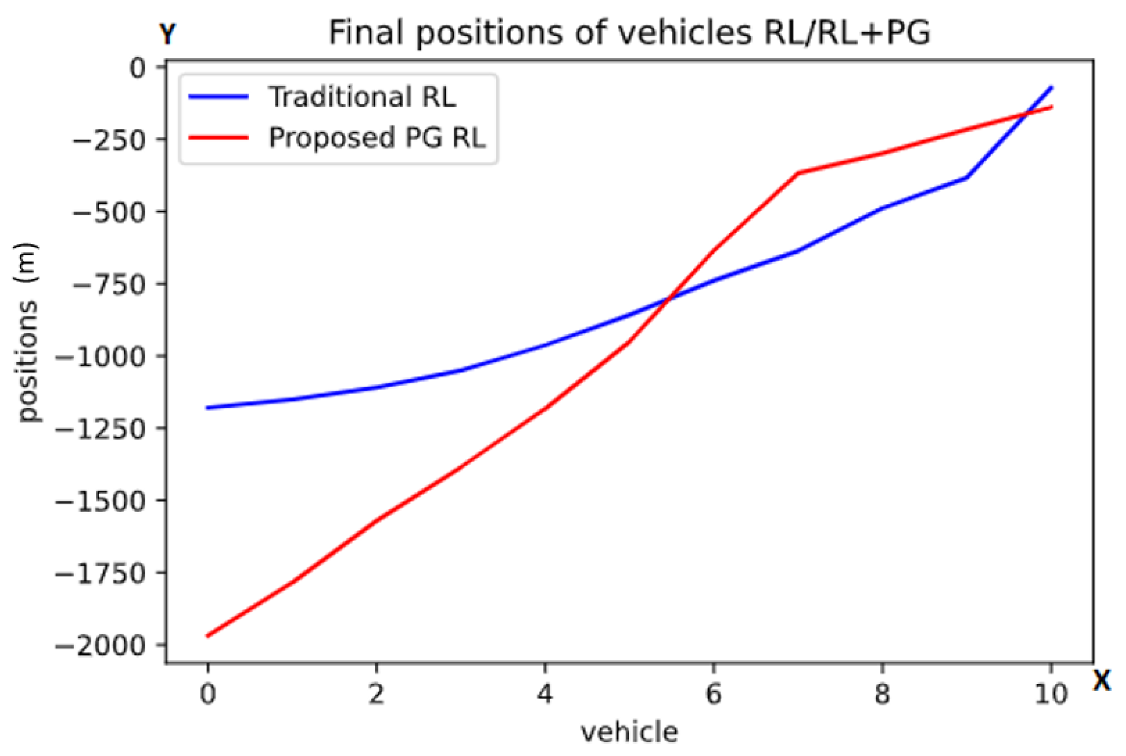
For the first task, it is important to mention that the first agent has no obstacles at all, nor a front vehicle to follow, this being a task to be learned by the other agents. Here, the acceleration of the lead vehicle will be / for 1100 steps, however, between steps 400 and 500 it will be at /. The lead vehicle will be followed by 11 agent-controlled vehicles initially separated by 20 m and with the initial velocities and accelerations being 0. In order to observe the difference between the two models we are evaluating, for simplicity, after 1100 steps we will capture the positions of the agent vehicles. Here, the chosen reward function is the constant collision penalization plus the reward r, leading to Equation (7):
The results of this task are presented in Figure 3.
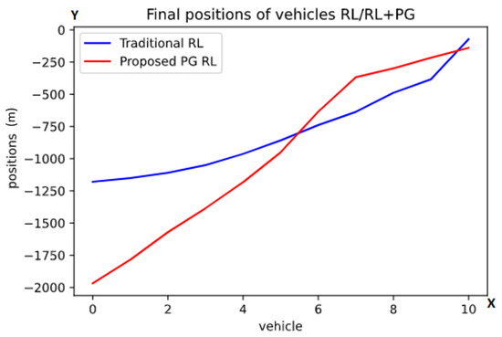
Figure 3.
Graph of the finals positions after the first task using the traditional RL (blue color) and the proposed PG RL (red color) models. The y-axis is representing the position behind the lead vehicle in meters while one point on the x-axis is referring to exactly one vehicle. These are the average final positions at the end of the scenarios, with the numbers referring to the vehicles (from back to front).
Here, the y-axis represents the position relative to the first agent and the x-axis represents the order of vehicles from the last one to the first one. For instance, if there is a point in the graph at x = 1 and y = 1000, that means that vehicle 1 ended 1000 m behind the first agent.
As can be observed in Figure 3, in the traditional RL model (blue color line), the final positions form a convex curve. In contrast, the proposed PG RL model (red color line) finds the agents spread more evenly than the traditional RL model. In order to put a magnitude to this appreciation of curvature/linearity in Figure 3, we calculated the distance of every point in the graphs to the corresponding points in a straight line connecting the first and the last point, this measure is also known as the Gini index. Then, we added the absolute values of these differences for each of the models and, as can be observed, our appreciation is correct, the sum of the distances being 1128 for the proposed PG RL model as compared to 1584 for the traditional RL model. While this doesn’t necessarily prove that one model is better than the other, it shows that the addition of physical knowledge in the model does have an effect on the behavior of the agents.
Next, we decided to study what would happen if there was some imprecision with the readings from the radar. To do this we introduce to each input a random uniform multiplier from 0.9 to 1.1. For example, if the real value of the reading were 10.0, the observed value would be a random value between 9.0 and 11.0 uniformly distributed. This randomness is applied to each input or simulated reading individually.
As we see in Figure 4 in comparison to Figure 3, we can observe that the perturbation of the inputs doesn’t change the innate behavior of the result for this task, but just smooths out each curve.
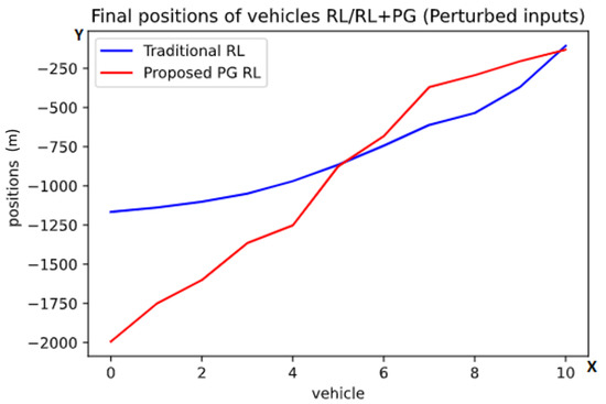
Figure 4.
Graph of the finals positions after the first task with randomized inputs using the traditional RL (blue color) and the proposed PG RL (red color) models. The y-axis is representing the position behind the lead vehicle in meters while one point on the x-axis is referring to exactly one vehicle. These are the average final positions at the end of the scenarios, with the numbers referring to the vehicles (from back to front).
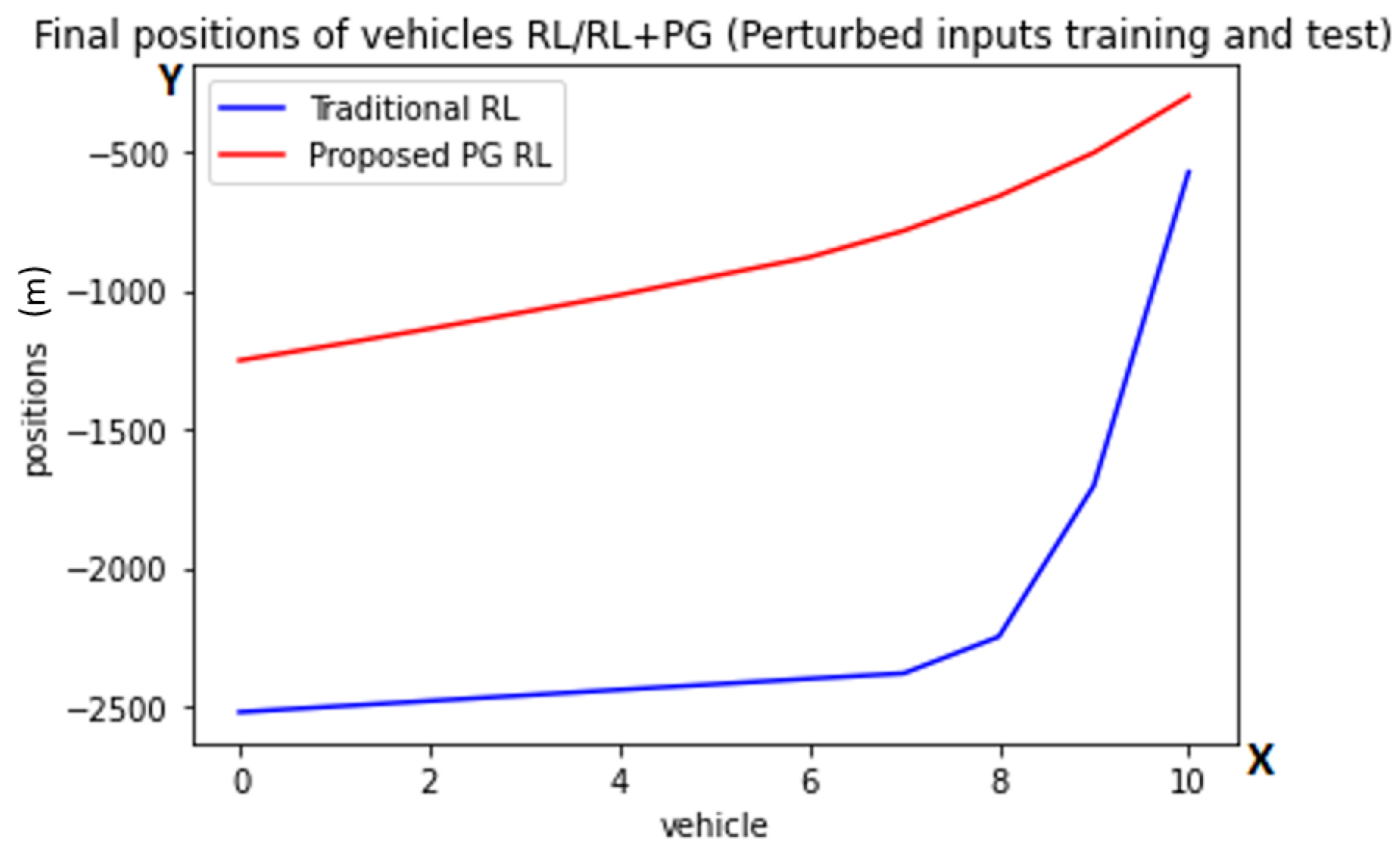
In Figure 5, we observe that the behavior of both models trained with perturbed inputs differs from its original counterparts. The average THW following a lead agent is of 21 s for the traditional model and 17 s for the PG RL model. This indicates a very slow behavior of the perturbed trained models, which is expected considering their experienced uncertainty. Lastly, we will reduce the number of agents to one in order to measure some of the criticality metrics introduced in [42] that apply to ACC such as HW, THW, and Deceleration to Safety Time (DST). The HW criticality metric (referenced as s in our work) is the distance between a vehicle and its leading vehicle.
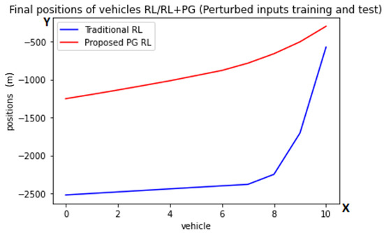
Figure 5.
Graph of the finals positions after the first task with randomized inputs using the traditional RL (blue color) and the proposed PG RL (red color) models trained with perturbations. The y-axis is representing the position behind the lead vehicle in meters while one point on the x-axis is referring to exactly one vehicle. These are the average final positions at the end of the scenarios, with the numbers referring to the vehicles (from back to front).
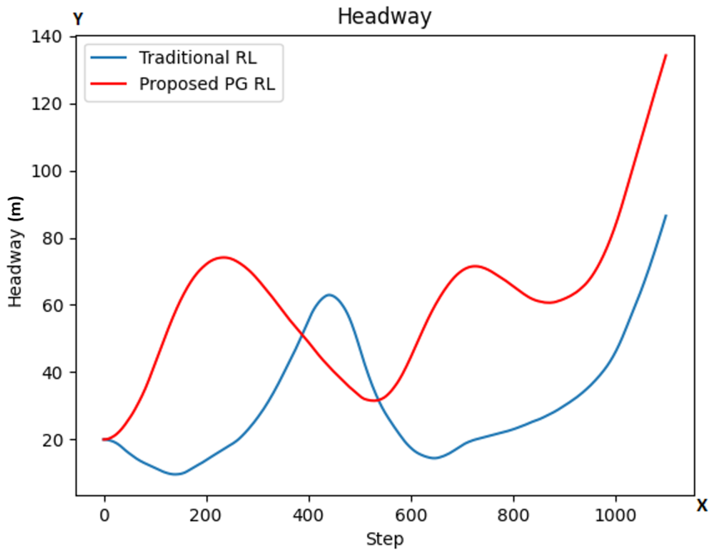
As we see in Figure 6, the HW in our proposed PG RL model (red color line) is at most steps higher than in the traditional RL model (blue color line), with its lowest points being also higher.
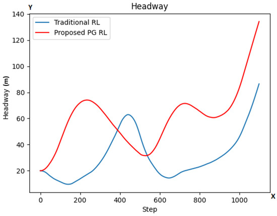
Figure 6.
HW values at each step for both models (traditional RL in blue color line; our proposed PG RL model in red color line). The y-axis is representing the HW values while the x-axis represents the number of simulation steps.
The THW criticality metric is the time a vehicle would take at a given step to reach its leading vehicle if its own velocity was constantly the same as the velocity at the given step and the leading vehicle remained still at its current position.
As we see in Figure 7, the THW in our PG RL model (red color line) is also at most steps higher than in the traditional RL model, with even its lowest points being higher. These results combined with the HW results suggest a more safe driving by our PG RL model than the traditional RL one.
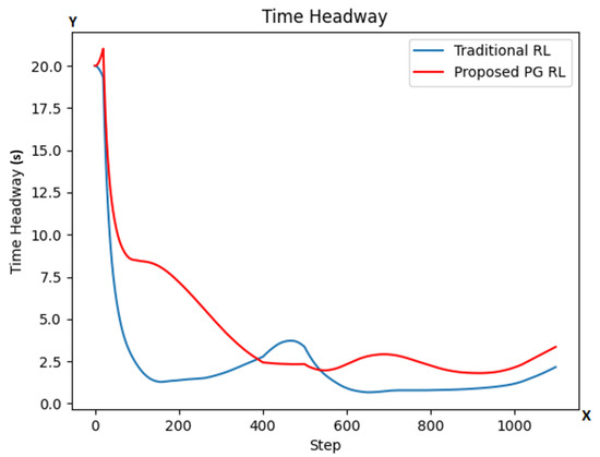
Figure 7.
THW values at each step for both models (traditional RL in blue color line; our proposed PG RL model in red color line). The y-axis is representing the THW values while the x-axis represents the number of simulation steps.
Finally, the DST metric calculates the deceleration required by the agent vehicle in order to maintain a safety time of seconds under the assumption of constant lead vehicle velocity. At a given step, the DST criticality metric is calculated as seen in Equation (8):
where is the agent’s velocity, is the lead vehicle’s velocity, and s is the distance between the vehicles, everything measured at a given step.
In Figure 8, we observe a strange behavior for both agents. The DST function spikes around steps 250, 550, and 1050. The values it reaches suggests impossible values for accelerations and decelerations, for instance requesting going from 400 m/s to 0 (at step 250) or from 0 to 300 m/s (at step 1050) in 0.1 s. The reason for these spikes is that the function for DST is linearly proportional to , which would suggest that the deceleration should be greater the closer the distance s is to , and more than that, that it should be infinite (with indeterminate sign) if , which, at the very least doesn’t coincide with the supposed objective of this function.
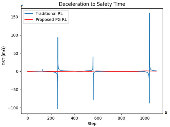
Figure 8.
DST values at each step for both models (traditional RL in blue color line; our proposed PG RL model in red color line). The y-axis is representing the DST while the x-axis represents the number of simulation steps.
5.2. Task 2
In the next tasks, the scenario will be the same as in Section 5.1, except that, here, we will introduce increasingly more dramatic brakes for the predetermined lead agent. More exactly, in the first of these tasks the deceleration rate will be /, in the second one, /, then / and finally /.
These considerations are very important for our evaluation because, for each of these tasks, we are able to observe which is the first agent vehicle that collides against the vehicle right in front of it, thus giving us a sense of how safe the platoon of vehicles is for both RL and PG RL models considered in this work. Thus, if the vehicle is the first vehicle that collides, we can say that the platoon is safe for vehicles in the given scenario.
As can be seen in Table 2, the proposed PG RL model is proving to be safer in every single scenario when compared to the traditional RL model.
Table 2.
Collision safety comparison between the traditional RL and the proposed PG RL models.
Here, the first column shows the deceleration of the lead agent in each scenario, with the second and third columns showing at each scenario which car was the first to c for each of the models respectively. The presented values in Table 2 come from testing the same scenario 20 times and obtaining the worst result.
We run the same experiment introducing perturbations to the inputs as in Section 5.1; however, since the agents were trained with perfect inputs, both of the models performed considerably worse. We did 20 attempts for each of the models and each of the lead deceleration values in Table 2, but no matter the number of vehicles, the first agent always collide against the lead vehicle in at least one of the 20 attempts.
Performing this experiment with the perturbed inputs, the trained models yield safer results due to the cautious nature of these models, however, this shouldn’t be taken as a virtue of these models because, upon qualitative analysis, we observe that they barely accelerate due to the uncertain nature of their training when compared to the regular trained ones.
6. Conclusions
Despite AI paving the way towards fully automated driving, its development is mostly driven by data without taking into consideration prior knowledge. This paper presents a novel approach in increasing the safety of ACCs by merging these two approaches, more exactly, by making use of physical knowledge in the form of jam-avoiding distance as part of a more processed input for a SAC RL algorithm. The advantage over constrained-based optimal control algorithms is that RL approaches do not require any data while the advantage over common rule-based driving is the greater flexibility of an RL-based agent thanks to the state abstractions learned by the underlying deep neural network. In our evaluation, we show that a PG RL agent is able to learn how to behave in its scenario better than a traditional RL approach, showing less collisions and more equidistant travel, providing a basis for future work to build upon. Another important result is the encouragingly good performance of our RL-based agents in the platooning scenario as well as in the scenario with perturbed input data. We want to emphasize that the agents do not have the opportunity to communicate but once one of the vehicles brakes, the vehicles behind it learn to brake as well by only observing the (perturbed) distance to the respective vehicle in front and their (perturbed) velocity. In addition, the proposed PG RL approach achieves considerable better results also when evaluated with criticality metrics such as TW and THW, proving that safety in AVs can be increased by making use of prior knowledge into AI components. As future work for improving the performance of an ACC, we plan to identify and integrate additional knowledge into the PG RL model by increasing the complexity of scenarios. We want to realize this by using additional traffic participants such as pedestrians crossing the road in front of the lead vehicle. Promising future directions are to consider adjacent domains such as Car2Car and Car2X communications which are able to provide information about better traffic predictions, as well as to integrate additional and diverse knowledge by other approaches such as extending the reward function.
Author Contributions
Conceptualization, S.L.J. and D.G.; methodology, S.L.J., D.G., T.W. and P.B.; software, S.L.J., D.G., P.B. and K.R.; validation, S.L.J., D.G., T.W. and E.M.; formal analysis, S.L.J., D.G., T.W. and P.B.; investigation, S.L.J., D.G., T.W., P.B., K.R. and E.M.; resources, S.L.J., D.G., T.W., P.B., K.R. and E.M.; data curation, S.L.J. and D.G.; writing—original draft preparation, S.L.J., D.G. and T.W.; writing—review and editing, S.L.J., D.G., T.W., P.B., K.R. and E.M.; visualization, S.L.J. and K.R.; supervision, E.M.; project administration, D.G., T.W. and E.M.; funding acquisition, E.M. All authors have read and agreed to the published version of the manuscript.
Funding
This work received funding from the German Federal Ministry of Economic Affairs and Energy (BMWi) through the KI-Wissen project under grant agreement No. 19A20020M.
Institutional Review Board Statement
Not applicable.
Informed Consent Statement
Not applicable.
Data Availability Statement
Not applicable.
Conflicts of Interest
The authors declare no conflict of interest.
Abbreviations and Nomenclature
The following abbreviations and symbols are used in this manuscript:
| ACC | Adaptive Cruise Control |
| ML | Machine Learning |
| SAC | Soft Actor-Critic Algorithm |
| RL | Reinforcement Learning |
| PG | Physics-guided |
| AI | Artificial Intelligence |
| AV | Autonomous vehicle |
| MRI | Magnetic Resonance Imaging |
| LIDAR | Light detection and ranging |
| IDM | Intelligent Driver Model |
| MDP | Markov decision process |
| HW | Headway |
| THW | Time Headway |
| DST | Deceleration to Safety Time |
| Soft Q-function | |
| State at time point t | |
| Action at time point t | |
| Soft Q-function parameter | |
| Policy with state-action pair | |
| Policy parameter | |
| Desired velocity | |
| T | Save time headway |
| Maximum acceleration | |
| b | Desired deceleration |
| Jam distance | |
| s | Distance to the leading vehicle |
| Minimum jam-avoiding distance | |
| v | Current agent velocity |
| Velocity difference to the leading vehicle | |
| t | Time point t |
| Velocity at time point t | |
| Acceleration at time point t | |
| Position at time point t | |
| h | Step size |
| State Space in MDP | |
| Action Space in MDP | |
| T | Deterministic transition model in MDP |
| r | Reward |
| Deterministic parametric policy | |
| Target seperation | |
| Deceleration to Safety Time | |
| Vehicle 1 | |
| Vehicle 2 |
Appendix A
Table A1.
Test results for the different combinations of parameters regarding the RL simulation.
Table A1.
Test results for the different combinations of parameters regarding the RL simulation.
| Model | Collisions | HW (m) | THW (s) | Separation (m) | |
|---|---|---|---|---|---|
| 0 | 0/predAcc/symmetric | 2 | 21.986616 | 4.746649 | 17.932934 |
| 1 | 0/predAcc/symmetric | 20 | 21.523313 | 4.598207 | 17.974341 |
| 2 | 0/predAcc/velocity | 20 | 12.238809 | 6.684551 | 17.714547 |
| 3 | 0/predAcc/absoluteDiff | 20 | 13.512952 | 7.932466 | 18.123747 |
| 4 | 0/predAcc/None | 10 | 552.604185 | 22.768953 | 21.750825 |
| 5 | 0/randomAcc/symmetric | 0 | 120.883542 | 5.407901 | 147.354975 |
| 6 | 0/randomAcc/velocity | 20 | 12.467875 | 7.977922 | 17.749884 |
| 7 | 0/randomAcc/absoluteDiff | 0 | 185.853298 | 8.008320 | 171.210850 |
| 8 | 0/randomAcc/None | 20 | 30.555453 | 4.365431 | 49.872451 |
| 9 | 0/randomStops9/symmetric | 10 | 111.509197 | 5.244257 | 17.899641 |
| 10 | 0/randomStops9/velocity | 20 | 17.324510 | 3.036292 | 13.902887 |
| 11 | 0/randomStops9/absoluteDiff | 20 | 13.116112 | 7.374774 | 17.958673 |
| 12 | 0/randomStops9/None | 0 | 818.533661 | 32.071159 | 229.345633 |
| 13 | 0/randomStops10/symmetric | 20 | 11.578542 | 2.877303 | 19.522080 |
| 14 | 0/randomStops10/velocity | 0 | 96.373722 | 4.650809 | 103.114341 |
| 15 | 0/randomStops10/absoluteDiff | 20 | 13.114346 | 7.399617 | 17.963344 |
| 16 | 0/randomStops10/None | 0 | 818.434954 | 32.064495 | 229.345483 |
| 17 | 100/predAcc/symmetric | 20 | 64.280247 | 7.214039 | 73.357278 |
| 18 | 100/predAcc/velocity | 20 | 12.276690 | 4.083880 | 13.097846 |
| 19 | 100/predAcc/absoluteDiff | 20 | 13.453637 | 7.653036 | 18.272531 |
| 20 | 100/predAcc/None | 10 | 795.550077 | 30.799090 | 22.119458 |
| 21 | 100/randomAcc/symmetric | 9 | 38.420217 | 2.480810 | 54.983419 |
| 22 | 100/randomAcc/velocity | 4 | 201.610520 | 7.274791 | 91.056809 |
| 23 | 100/randomAcc/absoluteDiff | 10 | 85.191944 | 4.217098 | 62.292352 |
| 24 | 100/randomAcc/None | 0 | 229.362628 | 10.193637 | 213.209962 |
| 25 | 100/randomStops9/symmetric | 0 | 88.737306 | 3.578192 | 89.672347 |
| 26 | 100/randomStops9/velocity | 20 | 9.988424 | 2.657730 | 13.041972 |
| 27 | 100/randomStops9/absoluteDiff | 20 | 12.637536 | 7.668094 | 17.778202 |
| 28 | 100/randomStops9/None | 0 | 794.717912 | 31.126503 | 229.345636 |
| 29 | 100/randomStops10/symmetric | 2 | 119.310468 | 5.001601 | 95.460083 |
| 30 | 100/randomStops10/velocity | 20 | 26.619944 | 4.218386 | 53.601016 |
| 31 | 100/randomStops10/absoluteDiff | 20 | 40.782619 | 4.782894 | 21.429448 |
| 32 | 100/randomStops10/None | 0 | 815.799968 | 31.938171 | 229.311862 |
| 33 | 3,000/predAcc/symmetric | 0 | 30.806897 | 2.256980 | 104.479287 |
| 34 | 3,000/predAcc/velocity | 18 | 16.539250 | 2.489905 | 10.804999 |
| 35 | 3,000/predAcc/absoluteDiff | 20 | 13.571941 | 4.840553 | 18.439911 |
| 36 | 3,000/predAcc/None | 0 | 800.393554 | 31.542861 | 229.345636 |
| 37 | 3,000/randomAcc/symmetric | 0 | 557.436259 | 21.370929 | 189.098820 |
| 38 | 3,000/randomAcc/velocity | 1 | 314.244283 | 11.907776 | 174.433635 |
| 39 | 3,000/randomAcc/absoluteDiff | 0 | 519.028676 | 19.635769 | 198.585035 |
| 40 | 3,000/randomAcc/None | 0 | 487.673884 | 18.984621 | 227.800876 |
| 41 | 3,000/randomStops9/symmetric | 0 | 121.610496 | 5.503739 | 145.529442 |
| 42 | 3,000/randomStops9/velocity | 0 | 71.099924 | 3.601645 | 96.712122 |
| 43 | 3,000/randomStops9/absoluteDiff | 20 | 12.240173 | 2.740492 | 16.209725 |
| 44 | 3,000/randomStops9/None | 0 | 736.721510 | 29.327481 | 229.345636 |
| 45 | 3,000/randomStops10/symmetric | 0 | 95.886739 | 4.443669 | 103.119817 |
| 46 | 3,000/randomStops10/velocity | 14 | 9.988159 | 4.999919 | 33.352000 |
| 47 | 3,000/randomStops10/absoluteDiff | 20 | 13.616155 | 6.805060 | 18.093497 |
| 48 | 3,000/randomStops10/None | 0 | 160.721774 | 7.162411 | 154.905059 |
| 49 | 100,000/predAcc/symmetric | 16 | 76.071190 | 3.418030 | 16.016787 |
| 50 | 100,000/predAcc/velocity | 1 | 134.614581 | 6.869882 | 149.200815 |
| 51 | 100,000/predAcc/absoluteDiff | 0 | 818.685845 | 32.077105 | 229.344549 |
| 52 | 100,000/predAcc/None | 0 | 761.794150 | 29.485078 | 229.345636 |
| 53 | 100,000/randomAcc/symmetric | 0 | 160.713442 | 8.460585 | 225.571123 |
| 54 | 100,000/randomAcc/velocity | 0 | 817.021321 | 31.972462 | 229.345213 |
| 55 | 100,000/randomAcc/absoluteDiff | 0 | 576.845622 | 23.913704 | 229.345636 |
| 56 | 100,000/randomAcc/None | 0 | 509.216830 | 21.192002 | 229.345242 |
| 57 | 100,000/randomStops9/symmetric | 0 | 90.975791 | 4.659583 | 135.021949 |
| 58 | 100,000/randomStops9/velocity | 0 | 76.346305 | 4.586848 | 130.914674 |
| 59 | 100,000/randomStops9/absoluteDiff | 0 | 292.012632 | 14.117718 | 229.345634 |
| 60 | 100,000/randomStops9/None | 0 | 816.244478 | 31.961323 | 229.345221 |
| 61 | 100,000/randomStops10/symmetric | 0 | 174.359445 | 7.620220 | 144.156391 |
| 62 | 100,000/randomStops10/velocity | 0 | 430.033252 | 18.551971 | 229.345570 |
| 63 | 100,000/randomStops10/absoluteDiff | 0 | 379.953210 | 16.932130 | 229.340859 |
| 64 | 100,000/randomStops10/None | 10 | 688.564158 | 26.086424 | 54.548802 |
References
- Singh, S. Critical Reasons for Crashes Investigated in the National Motor Vehicle Crash Causation Survey 2015. Available online: https://crashstats.nhtsa.dot.gov/Api/Public/ViewPublication/812115 (accessed on 24 October 2021).
- Ni, J.; Chen, Y.; Chen, Y.; Zhu, J.; Ali, D.; Cao, W. A Survey on Theories and Applications for Self-Driving Cars Based on Deep Learning Methods. Appl. Sci. 2020, 10, 2749. [Google Scholar] [CrossRef]
- Clements, L.M.; Kockelman, K.M. Economic Effects of Automated Vehicles. Transp. Res. Rec. 2017, 2606, 106–114. [Google Scholar] [CrossRef]
- Karpatne, A.; Watkins, W.; Read, J.S.; Kumar, V. Physics-guided Neural Networks (PGNN): An Application in Lake Temperature Modeling. arXiv 2017, arXiv:1710.11431. [Google Scholar]
- von Rueden, L.; Mayer, S.; Beckh, K.; Georgiev, B.; Giesselbach, S.; Heese, R.; Kirsch, B.; Walczak, M.; Pfrommer, J.; Pick, A.; et al. Informed Machine Learning—A Taxonomy and Survey of Integrating Prior Knowledge into Learning Systems. IEEE Trans. Knowl. Data Eng. 2021, 1. [Google Scholar] [CrossRef]
- Yaman, B.; Hosseini, S.A.H.; Moeller, S.; Ellermann, J.; Uğurbil, K.; Akçakaya, M. Self-supervised learning of physics-guided reconstruction neural networks without fully sampled reference data. Magn. Reson. Med. 2020, 84, 3172–3191. [Google Scholar] [CrossRef]
- Gumiere, S.J.; Camporese, M.; Botto, A.; Lafond, J.A.; Paniconi, C.; Gallichand, J.; Rousseau, A.N. Machine Learning vs. Physics-Based Modeling for Real-Time Irrigation Management. Front. Water 2020, 2, 8. [Google Scholar] [CrossRef] [Green Version]
- Zhang, Z.; Sun, C. Structural damage identification via physics-guided machine learning: A methodology integrating pattern recognition with finite element model updating. Struct. Health Monit. 2020, 20, 1675–1688. [Google Scholar] [CrossRef]
- Piccione, A.; Berkery, J.; Sabbagh, S.; Andreopoulos, Y. Physics-guided machine learning approaches to predict the ideal stability properties of fusion plasmas. Nucl. Fusion 2020, 60, 046033. [Google Scholar] [CrossRef]
- Muralidhar, N.; Bu, J.; Cao, Z.; He, L.; Ramakrishnan, N.; Tafti, D.; Karpatne, A. Physics-Guided Deep Learning for Drag Force Prediction in Dense Fluid-Particulate Systems. Big Data 2020, 8, 431–449. [Google Scholar] [CrossRef] [PubMed]
- Wang, J.; Li, Y.; Zhao, R.; Gao, R.X. Physics guided neural network for machining tool wear prediction. J. Manuf. Syst. 2020, 57, 298–310. [Google Scholar] [CrossRef]
- AI Knowledge Consortium. AI Knowledge Project. 2021. Available online: https://www.kiwissen.de/ (accessed on 24 October 2021).
- Wei, Z.; Jiang, Y.; Liao, X.; Qi, X.; Wang, Z.; Wu, G.; Hao, P.; Barth, M. End-to-End Vision-Based Adaptive Cruise Control (ACC) Using Deep Reinforcement Learning. arXiv 2020, arXiv:2001.09181. [Google Scholar]
- Kesting, A.; Treiber, M.; Schönhof, M.; Kranke, F.; Helbing, D. Jam-Avoiding Adaptive Cruise Control (ACC) and its Impact on Traffic Dynamics. In Traffic and Granular Flow’05; Schadschneider, A., Pöschel, T., Kühne, R., Schreckenberg, M., Wolf, D.E., Eds.; Springer: Berlin/Heidelberg, Germany, 2007; pp. 633–643. [Google Scholar]
- Kral, W.; Dalpez, S. Modular Sensor Cleaning System for Autonomous Driving. ATZ Worldw. 2018, 120, 56–59. [Google Scholar] [CrossRef]
- Knoop, V.L.; Wang, M.; Wilmink, I.; Hoedemaeker, D.M.; Maaskant, M.; der Meer, E.J.V. Platoon of SAE Level-2 Automated Vehicles on Public Roads: Setup, Traffic Interactions, and Stability. Transp. Res. Rec. 2019, 2673, 311–322. [Google Scholar] [CrossRef]
- Pathak, S.; Bag, S.; Nadkarni, V. A Generalised Method for Adaptive Longitudinal Control Using Reinforcement Learning. In International Conference on Intelligent Autonomous Systems; Springer: Cham, Switzerland, 2019; pp. 464–479. [Google Scholar]
- Farag, A.; AbdelAziz, O.M.; Hussein, A.; Shehata, O.M. Reinforcement Learning Based Approach for Multi-Vehicle Platooning Problem with Nonlinear Dynamic Behavior 2020. Available online: https://www.researchgate.net/publication/349313418_Reinforcement_Learning_Based_Approach_for_Multi-Vehicle_Platooning_Problem_with_Nonlinear_Dynamic_Behavior (accessed on 24 October 2021).
- Chen, C.; Jiang, J.; Lv, N.; Li, S. An intelligent path planning scheme of autonomous vehicles platoon using deep reinforcement learning on network edge. IEEE Access 2020, 8, 99059–99069. [Google Scholar] [CrossRef]
- Forbes, J.R.N. Reinforcement Learning for Autonomous Vehicles; University of California: Berkeley, CA, USA, 2002. [Google Scholar]
- Sallab, A.E.; Abdou, M.; Perot, E.; Yogamani, S. Deep Reinforcement Learning framework for Autonomous Driving. arXiv 2017, arXiv:1704.02532. [Google Scholar] [CrossRef] [Green Version]
- Kiran, B.; Sobh, I.; Talpaert, V.; Mannion, P.; Sallab, A.; Yogamani, S.; Perez, P. Deep Reinforcement Learning for Autonomous Driving: A Survey. IEEE Trans. Intell. Transp. Syst. 2021, 1–18. [Google Scholar] [CrossRef]
- Di, X.; Shi, R. A survey on autonomous vehicle control in the era of mixed-autonomy: From physics-based to AI-guided driving policy learning. Transp. Res. Part Emerg. Technol. 2021, 125, 103008. [Google Scholar] [CrossRef]
- Desjardins, C.; Chaib-draa, B. Cooperative Adaptive Cruise Control: A Reinforcement Learning Approach. IEEE Trans. Intell. Transp. Syst. 2011, 12, 1248–1260. [Google Scholar] [CrossRef]
- Curiel-Ramirez, L.; Ramirez-Mendoza, R.A.; Bautista, R.; Bustamante-Bello, R.; Gonzalez-Hernandez, H.; Reyes-Avendaño, J.; Gallardo-Medina, E. End-to-End Automated Guided Modular Vehicle. Appl. Sci. 2020, 10, 4400. [Google Scholar] [CrossRef]
- Li, Y.; Li, Z.; Wang, H.; Wang, W.; Xing, L. Evaluating the safety impact of adaptive cruise control in traffic oscillations on freeways. Accid. Anal. Prev. 2017, 104, 137–145. [Google Scholar] [CrossRef]
- Niedoba, M.; Cui, H.; Luo, K.; Hegde, D.; Chou, F.C.; Djuric, N. Improving movement prediction of traffic actors using off-road loss and bias mitigation. In Workshop on ’Machine Learning for Autonomous Driving’ at Conference on Neural Information Processing Systems. 2019. Available online: https://djurikom.github.io/pdfs/niedoba2019ml4ad.pdf (accessed on 24 October 2021).
- Phan-Minh, T.; Grigore, E.C.; Boulton, F.A.; Beijbom, O.; Wolff, E.M. Covernet: Multimodal behavior prediction using trajectory sets. In Proceedings of the IEEE/CVF Conference on Computer Vision and Pattern Recognition, Seattle, WA, USA, 13–19 June 2020; pp. 14074–14083. [Google Scholar]
- Boulton, F.A.; Grigore, E.C.; Wolff, E.M. Motion Prediction using Trajectory Sets and Self-Driving Domain Knowledge. arXiv 2020, arXiv:2006.04767. [Google Scholar]
- Cui, H.; Nguyen, T.; Chou, F.C.; Lin, T.H.; Schneider, J.; Bradley, D.; Djuric, N. Deep kinematic models for physically realistic prediction of vehicle trajectories. arXiv 2019, arXiv:1908.0021. [Google Scholar]
- Bahari, M.; Nejjar, I.; Alahi, A. Injecting Knowledge in Data-driven Vehicle Trajectory Predictors. arXiv 2021, arXiv:2103.04854. [Google Scholar] [CrossRef]
- Mohamed, A.; Qian, K.; Elhoseiny, M.; Claudel, C. Social-stgcnn: A social spatio-temporal graph convolutional neural network for human trajectory prediction. In Proceedings of the IEEE/CVF Conference on Computer Vision and Pattern Recognition, Seattle, WA, USA, 13–19 June 2020; pp. 14424–14432. [Google Scholar]
- Ju, C.; Wang, Z.; Long, C.; Zhang, X.; Chang, D.E. Interaction-aware kalman neural networks for trajectory prediction. In Proceedings of the 2020 IEEE Intelligent Vehicles Symposium (IV), Las Vegas, NV, USA, 19 October–13 November 2020; IEEE: Piscataway, NJ, USA, 2019; pp. 1793–1800. [Google Scholar]
- Chen, B.; Li, L. Adversarial Evaluation of Autonomous Vehicles in Lane-Change Scenarios. arXiv 2020, arXiv:2004.06531. [Google Scholar] [CrossRef]
- Ding, W.; Xu, M.; Zhao, D. Learning to Collide: An Adaptive Safety-Critical Scenarios Generating Method. arXiv 2020, arXiv:2003.01197. [Google Scholar]
- Qiao, Z.; Tyree, Z.; Mudalige, P.; Schneider, J.; Dolan, J.M. Hierarchical reinforcement learning method for autonomous vehicle behavior planning. arXiv 2019, arXiv:1911.03799. [Google Scholar]
- Li, X.; Qiu, X.; Wang, J.; Shen, Y. A Deep Reinforcement Learning Based Approach for Autonomous Overtaking. In Proceedings of the 2020 IEEE International Conference on Communications Workshops (ICC Workshops), Dublin, Ireland, 7–11 June 2020; IEEE: Piscataway, NJ, USA, 2020; pp. 1–5. [Google Scholar]
- Wu, Y.; Tan, H.; Peng, J.; Ran, B. A Deep Reinforcement Learning Based Car Following Model for Electric Vehicle. Smart City Appl. 2019, 2, 1–8. [Google Scholar] [CrossRef]
- Haarnoja, T.; Zhou, A.; Hartikainen, K.; Tucker, G.; Ha, S.; Tan, J.; Kumar, V.; Zhu, H.; Gupta, A.; Abbeel, P.; et al. Soft Actor-Critic Algorithms and Applications. arXiv 2019, arXiv:1812.05905. [Google Scholar]
- Hermand, E.; Nguyen, T.W.; Hosseinzadeh, M.; Garone, E. Constrained control of UAVs in geofencing applications. In Proceedings of the 2018 26th Mediterranean Conference on Control and Automation (MED), Zadar, Croatia, 19–22 June 2018; IEEE: Piscataway, NJ, USA, 2018; pp. 217–222. [Google Scholar]
- Wang, P.; Gao, S.; Li, L.; Sun, B.; Cheng, S. Obstacle avoidance path planning design for autonomous driving vehicles based on an improved artificial potential field algorithm. Energies 2019, 12, 2342. [Google Scholar] [CrossRef] [Green Version]
- Westhofen, L.; Neurohr, C.; Koopmann, T.; Butz, M.; Schütt, B.; Utesch, F.; Kramer, B.; Gutenkunst, C.; Böde, E. Criticality Metrics for Automated Driving: A Review and Suitability Analysis of the State of the Art. arXiv 2021, arXiv:2108.02403. [Google Scholar]
- Cassirer, A.; Barth-Maron, G.; Brevdo, E.; Ramos, S.; Boyd, T.; Sottiaux, T.; Kroiss, M. Reverb: A Framework For Experience Replay. arXiv 2021, arXiv:2102.04736. [Google Scholar]


Publisher’s Note: MDPI stays neutral with regard to jurisdictional claims in published maps and institutional affiliations. |
© 2021 by the authors. Licensee MDPI, Basel, Switzerland. This article is an open access article distributed under the terms and conditions of the Creative Commons Attribution (CC BY) license (https://creativecommons.org/licenses/by/4.0/).