A Flexible Top-Down Numerical Modeling of an Air-Cooled Finned-Tube CO₂ Trans-Critical Gas Cooler

Abstract

Carbon dioxide trans-critical refrigeration systems have been deeply investigated over the last years, with the aim to improve their performance by using several possible technical solutions. However, most of them lead to a more complex and expensive system, and therefore a trade-off is always needed to identify the best viable solution. Therefore, many efforts have also been focused on the study of a critical component of the basic carbon dioxide trans-critical cycle, which is the gas cooler, especially by numerical simulations. This work shows a new flexible approach to numerically model an air-cooled finned-tube CO₂ trans-critical gas cooler integrating a Top-Down methodology with a Finite Difference Method to solve the governing equation of the thermodynamic processes involved. The model was developed to reproduce the behavior of an experimental CO₂ refrigeration system, which provided the experimental data used for its validation. In detail, the model showed a good agreement with the experimental data, with average deviations of 1 K (0.3%), 0.9 bar (1%) and 0.15 kW (2.8%) regarding the refrigerant outlet temperature, the refrigerant outlet pressure and the rejected heat, respectively. The Top-Down numerical approach slightly outperformed the performance of previous numerical models available in the literature. Furthermore, the analysis of the refrigerant temperature and pressure along the tubes and rows also shows that the model can reproduce their behavior consistently and accordingly to data reported in the literature. The proposed approach can be used for detailed thermo-economic analysis of the whole refrigeration system, with the aim to optimize the design of the gas cooler.

1. Introduction

The refrigeration sector is currently characterized by a large utilization of hydro-fluorocarbon (HFC) refrigerants in most of the refrigeration systems all over the world. However, the growing concern about environmental issues regarding the global warming potential (GWP) of these working fluids led to some policy actions, such as the approval of the F-Gas Regulation [1] and the ratification of the Kigali amendment to the Montreal Protocol [2], which aim to phase out their utilization in the near future. Therefore, different technical solutions for refrigeration systems have been investigated over the last years. Among these, many researchers have been focused on the evaluation of the performance of alternative low-GWP refrigerants, including hydrocarbons (HC), such as isobutane (R600a) and propane (R290); natural refrigerants, such as carbon dioxide (R744) and ammonia (R717); hydro-fluoro-olefins (HFOs); and their mixture with HFCs, such as R1234yf, R1234ze, R450a and R513a among others [3,4,5,6,7]. The main target of the last studies about these possible replacements was to investigate the performance of these fluids as refrigerants and potential improvement which could increase them with the aim to get closer to the performance of HFC refrigerants, ensuring comparable cost with current solutions. The latter should facilitate the widespread acceptance of these alternative fluids.

Among alternatives low-GWP refrigerants, carbon dioxide is the only refrigerant that is non-flammable and non-toxic, with an Ozone Depletion Potential (ODP) equal to 0 and a negligible GWP (GWP = 1). It can work with temperatures below 0 °C, and it is classified as an A1 refrigerant [8]. Furthermore, carbon dioxide is also inexpensive and shows higher latent heat, specific heat, density and thermal conductivity and lower viscosity than HFCs. However, the application of carbon dioxide as a refrigerant usually requires a trans-critical cycle to properly reject heat to the ambient, and therefore, it requires high working pressures, which can limit its performance and require special design, manufacturing and control. The first application of a CO₂ trans-critical cycle was proposed and developed in 1990 by Lorentzen [9]. Then, the results regarding the performance of the first prototype for a car air-conditioning system were published three years later [10]. In the latter work, a comparison between the CO₂ trans-critical cycle and the conventional sub-critical refrigeration cycle was also carried out, showing lower performance of the former cycle, as further demonstrated later on by Sarkar [11], who compared carbon dioxide with several refrigerant fluids, such as ammonia, propane and R134a among others, highlighting COP values of about 40–50% smaller than the common applications.

Therefore, the last two decades of studies about CO₂ refrigeration systems were strongly focused on the investigation of possible methods and technical solutions to improve the performance of such systems, with the aim to make carbon dioxide competitive with other refrigerants. A very recent work reviewed the state-of-the-art of trans-critical CO₂ air conditioning and refrigeration technologies, considering both stationary and mobile applications, highlighting the basic characteristics of the common cycle and then discussing the possible modifications proposed over the years to improve its performance [12]. The authors concluded by stating that, even if a large amount of work has been performed on the development of individual components for the modification of the CO₂ trans-critical cycle, there still is much room for improvement, especially considering the advanced design and analysis tools available nowadays and the growing interest of the scientific community. Several technical solutions to improve the performance of the CO₂ trans-critical cycle were deeply investigated in the review by Yu et al. [13], where recent advances in the modification of such a cycle are emphasized and comprehensively discussed. In detail, the authors identified ten different technical solutions which can lead to different enhancements of the performance of the CO₂ trans-critical cycle, such as the use of an internal heat exchanger (IHX), an ejector, a vortex tube, an expander, subcooling techniques, a flash-gas bypass, a parallel compression, a two-stage compression, an evaporative precooling and CO₂-base mixtures. They highlighted the range of COP (Coefficient of Performance) improvement for each solution, pointing out the best candidates according to a comprehensive evaluation of their strength and weakness, such as cost, plant complexity, plant control and risks, among others. Another specific work about improvement methods for the CO₂ trans-critical cycle was presented by Llopis et al. [14], who focused the attention on different techniques to obtain the subcooling of the CO₂ exiting from the gas cooler of the plant. They discussed the advantages and disadvantages of using internal methods, such as an IHX, an economizer, an integrated mechanical sub-cooler and a heat storage system, or dedicated subcooling methods, such as a dedicated mechanical subcooling, a thermoelectric subcooling system and other hybrid systems, to obtain the desired subcooling degree. In the end, they mapped out some guidelines for future investigations and highlighted that there is a strong need of works regarding the possibility to optimize such subcooling methodologies, including sizing aspects, related to the overall dimension of the system and thermo-economic analysis. Indeed, recently, Aranguren et al. experimentally investigated the optimum working point of a CO₂ trans-critical cycle coupled with a thermo-electric subcooling system [15]. On the other hand, Cortella et al. performed a thermo-economic analysis of a CO₂ trans-critical cycle coupled with a dedicated mechanical subcooling system, highlighting the importance of the optimization, in terms of size and control, of this latter component [16]. In a similar way, Nebot-Andrés et al. experimentally optimized the working conditions of a CO₂ trans-critical cycle coupled with a R152a dedicated mechanical subcooling system, in terms of optimal gas cooler pressure and subcooling degree, and proposed two general correlations to determine the optimum gas cooler and intermediate pressure of a CO₂ trans-critical cycle with parallel compression [17,18].

Although many researchers are investigating these technical methods to improve the performance of CO₂ trans-critical cycles, also trying to optimize the working conditions of each specific solution, there is still the need to further characterize and improve one of the main components of the basic CO₂ trans-critical cycle, which is the gas cooler, where the carbon dioxide cools down, rejecting heat to the heat sink. In a CO₂ trans-critical refrigeration cycle, a finned-tube gas cooler has been widely used due to its simple geometry, durability, size and cost-effectiveness characteristics. Therefore, several experimental and theoretical investigations have been performed over the past two decades, with the aim to fully characterize such a component by considering the heat-transfer and friction behavior of the fluid. The latter is fundamental to optimize the operations of the device, and therefore optimize the performance of the whole system. In 2005, Erek et al. [19] investigated the influence of the changes in the fin geometry on heat transfer and pressure drop of a plate fine and tube heat exchanger by a CFD (Computational Fluid Dynamics) model. In detail, they focused on the effects of finned tube center location, fin height, tube thickness and ellipticity, and distance among fins on the heat transfer between the fluid flowing into the tubes and water, as well as on the pressure drop. Another CFD model regarding annular finned tubes was also proposed by Bilirgen et al. [20] to evaluate the effects of the fin spacing, fin height, fin thickness and fin material on the overall heat transfer and pressure drop for a single row of finned-tube. A comprehensive analysis of experimental and numerical studies about finned-tube heat exchangers was performed by Bhuiyan and Islam [21], who pointed out existing and emerging technologies and trends in designing finned-tube heat exchangers, considering different geometric parameters and arrangement. Even if these studies dealt with a generic finned tube heat exchanger, the results stemming from them can be applied also to a finned-tube gas cooler. Specifically concerning finned-tube gas coolers, a detailed steady-state mathematical model of an air-cooled finned-tube CO₂ gas cooler, using a distributed method to accurately predict the variation of both refrigerant thermophysical properties and local heat-transfer coefficients, was presented by Ge and Cropper [22]. The proposed modeling method allowed the authors to carry out some performance analysis with different circuit arrangements and structure parameters of the gas cooler, whereas the modeling distributed approach was necessary to accurately predict the large variation of the thermophysical properties of the refrigerant and the local heat-transfer coefficient expected during the gas cooling process. The model was validated with data available in the literature, showing an error regarding the refrigerant outlet temperature of about ± 2 K. Gupta and Dasgupta [23] analyzed a trans-critical CO₂ refrigeration system in typical Indian ambient conditions by modeling the air-cooled finned-tube gas cooler by using the Finite Difference Method (FDM), in which the three-dimensional geometry of the gas cooler is divided into a number of small elements, which consist of small tube section with a certain amount of fins. The numerical model was used to analyze the performance of the whole refrigeration system with different design and, especially, operating conditions, with the aim to identify the best possible performance. The gas cooler model was validated by using data from the available literature, showing deviations between the simulated and experimental refrigerant outlet temperature in the range between 0.2 and 4 K. Another CFD model of a finned-tube gas cooler was developed by Santosa et al. [24], with the aim to investigate the local refrigerant and air heat-transfer coefficients and how they are affected by the use of split fins. Furthermore, they proposed some correlations for overall refrigerant and air heat-transfer coefficients that can be used for system modeling. The developed model was validated against experimental data regarding the rejected heat and the air-outlet temperature, showing a good agreement between the experimental and simulated data. In the same year, Li et al. [25] proposed a new type of aluminum heat exchanger with integrated fins and micro-channel. They developed a steady-state segment-by-segment model to simulate the behavior of this type of gas cooler obtaining deviations of 5% and 8% in comparison with experimental data regarding the heat capacity and the refrigerant pressure drop, respectively. The proposed model was used to analyze the effects of fin geometry and mal-distribution of air on the performance of the device. The authors stated that the proposed heat exchanger has many advantages, such as high heat-transfer efficiency, simple processing and low cost, among others. One year later, another tri-dimensional CFD model of a CO₂ gas cooler was developed by adopting an equivalent approach to reduce the computational effort during the simulation and allow us to reproduce the effects of an extended finned surface [26]. The latter model was validated by considering experimental data from the available literature, providing good results in terms of heat rejected (deviation of about 2.5%) and temperatures (maximum deviation of about 3.8 K). Recently, the effect of uniform and mal-distribution inlet airflow profiles on the performance of a finned-tube CO2 gas cooler was investigated by a three-dimensional CFD model [27], especially considering the prediction of the refrigerant temperature profile along the tubes at different operating conditions. In detail, the influence of different airflow profiles, such as uniform, linear-up, linear-down and parabolic, on the heat-transfer coefficients, both air and refrigerant side, refrigerant temperature profile, air-pressure drop and rejected heat, was studied. The numerical model was validated by considering the refrigerant outlet temperature, providing a maximum deviation from the experimental data of about 3 K. The results showed that the airflow profile can have a strong impact on the performance of the gas cooler, especially considering the refrigerant temperature profile, and therefore the rejected heat. Still, another recent study aimed to quantify the effect of the heat conduction through fins of a finned-tube CO₂ gas cooler by CFD modeling obtained by an integration of both one-dimensional and three-dimensional models [28]. The one-dimensional model was developed to predict the refrigerant side heat-transfer process, whereas the three-dimensional model was built to evaluate the external airside heat-transfer process. The simulated results showed good agreement with empirical correlations and experimental data from the available literature, with temperature deviations within 5 K.

The CFD models demonstrated their capability to be effectively used for predicting the performance of a CO₂ trans-critical gas cooler, showing acceptable agreement with experimental data. Several researchers used CFD to investigate the effect of different parameters, especially regarding the geometry of the fins, on the performance of such a device and on the whole CO₂ refrigeration system. Then, more in-depth analyses were carried out to also analyze the effect of the airflow profile and the heat conduction through the fins, which can have a negative influence on the performance of the system. However, there is still a need to focus more on the development of numerical models using different approaches, with the aim to highlight different aspects which can lead to optimize the working operations of the gas cooler and improve the overall performance of the refrigeration system. Furthermore, the numerical models developed so far are mainly focused on the core part of the gas cooler, which consists of the finned-tubes where the refrigerant flows and reject heat to the air. Anyway, the analysis of the inlet and outlet side of the gas cooler, as well as of the air side structure, composed by the fan and a hypothetical diffuser with a grid, can lead to identify new paths to optimize the working operations of the gas cooler, especially considering that the structure of the air side compartment (hereinafter called fan compartment) affects the flow profile of the air investing the finned-tubes where the refrigerant flows. Therefore, this work proposes a new flexible numerical model of a CO₂ trans-critical gas cooler developed by a Top-Down approach, consisting of a step-by-step decomposition of the device into different parts until achieving a basic computational element where the governing equations of the heat and mass transfer are solved by the FDM. The proposed methodology highlights each essential part of the gas cooler from a geometrical point of view, and it would allow us to deeply analyze the effect of any geometrical modification on its performance according to defined working conditions, helping to identify the optimal geometrical design. This work represents one of the first attempt to decompose the structure of a CO₂ trans-critical gas cooler by using a Top-Down approach with the aim to address some design issues regarding both its core part, represented by the tubes where the heat exchange occurs, and its side parts, such as the fan compartment and the diffuser, which can strongly affect the performance of such a device since they can modify the inlet airflow distribution. In detail, the flexibility of the model allows us to evaluate several possible configurations of the gas cooler, considering different number of circuits, rows per circuit and tubes per circuit, as well as their arrangement within the heat exchanger by changing the values of the wheelbases (along two different directions). Moreover, the model allows us to change the inlet airflow distribution, with the aim to evaluate the performance for different system designs. So far, only one study focused on the effect of the airflow distribution on the performance of a gas cooler, highlighting the importance of such a parameter [27]. Here, the use of an experimental inlet airflow distribution allowed the authors to improve the accuracy of the predictions in comparison with a uniform airflow distribution, which is commonly used for gas-cooler modeling. The numerical model was developed to reproduce the working operations of a CO₂ refrigeration experimental plant [29], and it was validated by using the experimental data stemming from it regarding the refrigerant outlet temperature, refrigerant outlet pressure and rejected heat. The presented results ensure the good capability of the numerical model to predict the performance of the gas cooler, showing a better accuracy in comparison with previous models. The Top-Down approach presented in this work can open new ways to improve the performance of the gas cooler, and it could be used for a detailed thermo-economic analysis of the whole system, with the aim to optimally design each part of it. Indeed, it was developed with the aim of emphasizing the possibility to optimize the design of such a device, considering its core and side components, which both strongly affect its performance, acting on the refrigerant and air side, respectively.

2. Experimental Setup

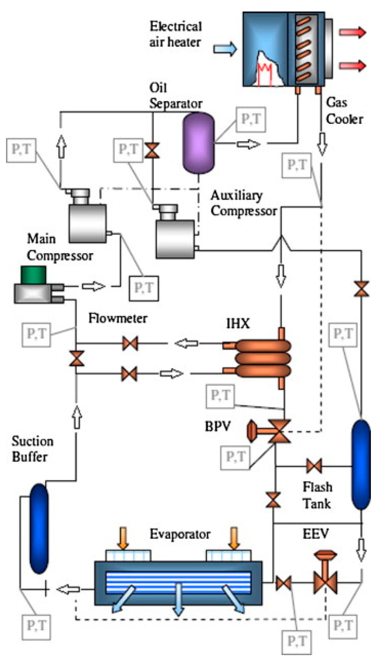
The experimental setup used to obtain the experimental data for the validation of the numerical model proposed in this work is shown in Figure 1. It is composed by four main components, which are two single-stage semi-hermetic reciprocating compressors, an air gas cooler, an air evaporator and an electronic expansion valve (EEV). In addition, the experimental plant is completed by an oil separator after the compressors, a liquid receiver after the gas cooler and an electronic back pressure valve (BPV), which is needed to keep a constant pressure of the refrigerant exiting the gas cooler.

The main compressor works in a pressure range between 15 and 120 bar, whereas the auxiliary compressor works between 55 and 120 bar. Both compressors have a nominal power of 2.5 kW. An internal heat exchanger (IHX) was also designed and installed in the experimental setup to study its effect on the performance of the plant. However, the latter was already discussed in a previous work [29], and it is not the aim of this study. The lamination process is performed by the electronic expansion valve, together with the back-pressure valve. The air gas cooler is characterized by four circuits (each one with one supply tube), three rows for each circuit and 5 tubes for each row. The copper tubes are characterized by several aluminum fins, with a depth of 0.15 mm and a pitch of 2.7 mm. On the other hand, the air evaporator is characterized by one circuit, eleven rows and six tubes for each row. As in the case of the gas cooler, the copper tubes are characterized by several aluminum fins, with a depth of 0.7 mm and a pitch of 3.5 mm. Furthermore, some electrical resistances were placed in the inlet channel of the air flow, which was thermally insulated. The latter allowed us to modify the inlet air temperature of the gas cooler to simulate different ambient conditions.

Different sensors were used to evaluate the performance of the plant and each component, especially considering the gas cooler. Indeed, temperature and pressure sensors were placed at the inlet and the outlet of each component. In detail, temperatures were measured by four-wire PT100 thermo-resistances with an accuracy of 0.15 °C. These sensors were placed on the inlet and outlet tubes, using a layer of a heat-transfer compound (aluminum oxide with silicon) to provide good thermal contact. Moreover, tubes were insulted with 25 mm of thick flexible insulation. Piezoelectric sensors were used to measure the pressure value at the inlet and the outlet of each component. They provide a current output directly recorded on a data logger. They were calibrated in the range of 0–100 bar gauge with an accuracy of 0.4%. A mass flowmeter was set up on the suction line of the main compressor to measure the refrigerant mass flow rate, and since it could be affected by the device vibration during normal operations, it was mounted on a 25 kg steel plate, located away from the plant. A power meter was used to measure the electrical power supplied to the compressors characterized by an accuracy of 0.2% in the range between 0.5 and 6 kW. The data acquisition was carried out with an A/D converter acquisition card, which allows a high sampling rate, and a personal computer, which allowed us to monitor and collect all measurements acquired by the sensors, using a data acquisition software realized in the LabView environment.

All experimental tests were performed in steady-state conditions, with the aim to have a set of experimental data to validate the model developed for the gas cooler. For this reason, temperature and pressure values were continuously monitored to check the achievement of the steady-state condition. In detail, it was assumed that the steady-state condition was achieved when the variations of all monitored variables from their corresponding average values are lower than 0.5 °C and 0.5 bar for temperatures and pressures, respectively. Once achieved, the steady-state condition, the test starts and the experimental data are recorded with a frequency of 0.5 Hz for 60 s. For each measured variable, the samples recorded are averaged. Then, after 180 s, each sample is checked again for other 60 s and compared to the previous corresponding average values: when the difference in the average values of temperatures and pressures are below than the defined ranges, the steady-state is achieved and the experimental data are fixed for the specific test.

The procedure described above allowed us to obtain the experimental data of temperature and pressure needed to characterize the entire plant and each specific component. However, only the experimental data regarding the temperatures and pressures at the inlet and outlet of the gas cooler are considered in this work, since they are necessary to validate the presented numerical model.

3. Numerical Modeling

The numerical model developed to describe the operations of the air-cooled finned-tube CO₂ gas cooler is based on the Top-Down approach, which allows us to obtain the performance of such a device, starting from a macroscopic point of view, and subsequently investigating more in-depth each part of the system, describing it as an ensemble of basic computational elements. It means that the system, which can be seen as a black-box, is gradually decomposed in simpler elements, thus allowing for a deeper investigation of the thermodynamic processes involved. In detail, the finned-tube CO₂ gas cooler is decomposed into four different levels (Figure 2), which are different from each other regarding the level of investigation. The first level is composed by the gas cooler seen as a black-box. Then, it is decomposed in three parts (second level): upstream structure, core structure and downstream structure. The former and the latter represent the inlet and the outlet of the gas cooler, whereas the core structure is its key part, where the main thermodynamic processes take place. Therefore, the core structure is further decomposed in three other parts (third level): fan compartment, diffuser and tubes. In the end (fourth level), the basic computational element is represented by a portion of the finned-tubes (hereinafter called finned cell) in which every thermodynamic property is defined for both the refrigerant and air.

The mathematical problem solved for each finned cell is characterized by the conservation equation of mass (Equation (1)), momentum (Equation (2)) and energy (Equation (3)), referred to the refrigerant, considering the hypotheses of homogeneous model [30,31,32], with the following assumptions:

• The refrigerant flow is considered one-dimensional, pure (no oil contamination) and incompressible;
• The variations of the kinetic and potential energies are negligible;
• The air exchanges heat power with a finned surface and a fin efficiency is considered;
• The axial conduction within the pipe wall is ignored;
• The air heat transfer coefficient is uniform and no mass and energy accumulation occurs treating the air as incompressible;
• The model is developed under steady-state conditions;
• One-dimensional flow, with refrigerant moving along the x-direction and the air moving along the y-direction;
• The refrigerant is considered as a pure substance, without oil contamination.

$$\frac{\mathrm{d}}{dx}\left(\rho u\right)=0,$$

(1)

$$\frac{\mathrm{d}}{dx}\left(\rho u^2\right)=-\frac{d}{dx}p+F_x,$$

(2)

$$\frac{\mathrm{d}}{dx}\left(\rho uh\right)=\frac{4}{D_i}{U}_{ref}\left(T_{ref}-T_{wall}\right),$$

(3)

where $\rho$ is the density in kg m⁻³$, u$ is the speed in m s⁻¹$, p$ is the pressure in Pa, $F_x$ is the pressure drop in Pa m⁻¹$, h$ is the enthalpy in J kg⁻¹$, D_i$ is the inner diameter of the tube in m, $U_{ref}$ is the heat transfer coefficient of the refrigerant in W m⁻²K⁻¹$, T_{ref}$ is the temperature of the refrigerant in K and $T_{wall}$ is the temperature of the tube wall in K.

Then, considering the balance equation on the wall of the tube, another equation is added to the previous set of equations, as follows:

$$U_{air}\frac{A_{air,eff}}{c_{p,air}}\left(h_{air,wall}-h_{air}\right)=U_{ref}{A}_{int}\left(T_{ref}-T_{wall}\right),$$

(4)

where $U_{air}$ is the heat transfer coefficient of the air in W m⁻²K⁻¹$, A_{air,eff}$ is the effective external heat transfer surface in contact with air in m²$, c_{p,air}$ is the specific heat of air in J kg⁻¹K⁻¹$, h_{air}$ is the enthalpy of the air in J kg⁻¹, $h_{air,wall}$ is the enthalpy of the air with a temperature equal to the wall temperature in J kg⁻¹ and $A_{int}$ is the internal surface of the tube.

Since the system of equations represented by Equations (1)–(4) is characterized by five different unknowns ($T_{ref}$, $T_{wall}$, $T_{air}$, ${\rho }_{ref}$ and $u_{ref}$), and therefore a further equation should be required, the iterative bisection method was used to find the solution of the mathematical problem. The whole numerical model was implemented in the MatLab environment, using RefProp software for the evaluation of the thermodynamic properties of the refrigerant [33].

3.1. The First Level

The gas cooler, representing the first level of the Top-Down model proposed, is one of the main components of a CO₂ trans-critical cycle, and it allows us to cool the superheated refrigerant by rejecting heat to the heat sink. In the investigated case, the heat rejection occurs by forced convection with air moved by a fan in a cross-flow direction in respect to the refrigerant flow. Schematically, the gas cooler can be seen as a black-box where the refrigerant enters with a specific mass flow rate (${\dot{m}}_{ref,in}$) and a specific inlet temperature ($T_{ref,in}$) and pressure ($P_{ref,in}$); rejects heat to the air crossing the heat exchanger with a specific mass flow rate (${\dot{m}}_{ref,in}$), which depends on the geometry of the fan and the air speed ($u_{air,in}$), at the ambient temperature ($T_{air,in}$); and, in the end, exits with mass flow rate (${\dot{m}}_{ref,out}$), outlet temperature ($T_{ref,out}$) and pressure ($P_{ref,out})$, as shown in Figure 3.

To evaluate the thermodynamic properties of the refrigerant exiting the gas cooler, as well as the temperature of the air exiting the gas cooler ($T_{air,out}$), the gas cooler is divided into three main parts, which are as follows:

• Upstream structure, composed by the tube which leads the refrigerant into the gas cooler and its connected manifold;
• Core structure, consisting of the actual heat exchanger;
• Downstream structure, composed by the outlet manifold and the tube which leads the refrigerant out of the gas cooler.

Therefore, the first level, which does not involve any calculation, is built as an input level to provide the model with all of the data needed to evaluate the thermodynamic processes occurring in the levels before, especially in the core structure. In detail, the geometry of the heat exchanger and the inlet thermodynamic properties of both the refrigerant and air are defined in this level. Some details about the calculations performed in the first level are provided in Appendix A.1.

3.2. The Second Level

In Figure 4, the structure of the second level of the numerical model is shown, starting from the upstream to the downstream structure, going through the core structure.

The upstream structure (Figure 4a) is composed by the inlet tube connected to the manifold, which is needed to spread the fluid flow among the different circuits of the heat exchanger that total four in the investigated case. The number of circuits is a design parameter, and it can be changed to analyze its effect on the performance of the gas cooler. The upstream structure is characterized by the conservation equation of mass, as follows:

$${\dot{m}}_{ref, in}={{\displaystyle \sum }}_{i=1}^{N_{sup}}{ \dot{m} }_{ref, i},$$

(5)

where ${\dot{m}}_{ref, i}$ is the refrigerant mass flow rate in the i-th circuit. Assuming an adiabatic process, and therefore neglecting the natural convection, we see that the temperature of the refrigerant in each circuit is equal to the inlet temperature of the refrigerant, as well as the pressure. The upstream structure simply considers the geometry of the gas cooler described in the first level as an input to provide the mass flow rate, temperature and pressure of the refrigerant within each circuit as outputs.

The core structure (Figure 4b) represents the element where all the important thermodynamic processes occur. It is characterized by four supply tubes (which can be changed according to the needs), which are the outlet of the upstream structure, a central body consisting of the actual heat exchanger, and four discharge tubes, which are the inlet for the downstream structure. Since most of thermodynamic processes take place in the core structure of the gas cooler, it is further divided into three sub-elements, i.e., the fan compartment, diffuser and tubes, composing the third level of the model.

The downstream structure (Figure 4c) is the specular component of the upstream structure, and it is characterized by the discharge tubes exiting by the core structure, a manifold, which brings together the different refrigerant flows by adiabatic mixing, and the outlet tube of the gas cooler, which leads the refrigerant to the expansion element. The mass flow rate of the refrigerant exiting the gas cooler is calculated as shown in Equation (5). Instead, its thermodynamic properties, which represents the output of the entire numerical model, are calculated as a weighted average of the different mass flow rate in each discharge tube. In the end, the rejected heat is also evaluated. The thermodynamic properties of air exiting the gas cooler are also evaluated in this stage, especially the enthalpy and temperature. The details of the calculation are shown in Appendix A.2. The air outlet temperature ($T_{air,out}$) is calculated by using the iterative bisection method in the interval [$T_{air,in}$, $T_{ref,in}$] and considering that the enthalpy of air can be evalauted as the product between the temperature and the specific heat. See Appendix A.3 for more details about the iterative method adopted.

The downstream structure, even if it does not involve the main thermodynamic processes, plays a key role into the numerical model, since it evaluates and provides its overall outputs. However, as said before, the core structure is much more important to understand what happens inside the gas cooler, and therefore it was further divided into three sub-elements.

3.3. The Third Level

Figure 5 shows the scheme of the third level of the numerical model, which is a further decomposition of the core structure (see Figure 2), composed by the fan compartment, the diffuser and the compartment where the tubes are arranged.

The fan is characterized by two main parameters, which are the mass flow rate and the pressure. The fan compartment is completely defined by two more design parameters: diameter of the section, which allows us to calculate the area of the inlet section; and the average speed of the air at the inlet of the compartment. The latter is fundamental, since it allows us to evaluate the mass flow rate of the air flowing towards the tubes through the diffuser, as in Equation (A3), where the mass flow rate of the air is evaluated by considering the presence of the electrical motor of the fan and the grid.

The diffuser increases the area of the air-transition section, allowing the airflow to invest all tubes of the heat exchanger. However, the airflow cannot be completely developed, since the length of the diffuser (distance between the outlet section of the fan compartment and the first rows of tubes) is very small. Therefore, the diffuser element is considered to include in the numerical model two different distributions of mass flow rate of the air at the outlet section: a uniform distribution, which assumes that the air speed is the same for each point of the outlet section; and an experimental distribution, which is derived from PIV experimental data by Marinetti et al. [34]. In the end, the diffuser, which can be seen just as a connection between the fan compartment and tubes, provides the air mass flow rate investing every finned cell of the tubes.

The arrangement of the tubes is shown in Figure 6. In detail, the front view (Figure 6a) shows the separation between the portion of tubes without fins (free tube) and the portion of the heat exchanger with finned-tubes (in the middle), whereas the side view (Figure 6b) highlights the structure of the gas cooler, organized with four different supply tubes, each of them with three rows of five tubes. The latter leads to a total number of fifteen jointed tubes per each circuit.

It is worth highlighting that only the finned-tubes take part to the heat rejection by forced convection, whereas the free tubes reject heat by natural convection. Tubes are characterized by several design parameters, such as the material, which affects the thermal conductivity of the tube; the external diameter; the thickness; and the length. Furthermore, from a computational point of view, it is also needed to define two more variables to define the path which the refrigerant follows along the supply tubes and the tubes for each supply tube. However, all these parameters are defined at the first level of the numerical model, as already described in Section 3.1.

Since this element represents the core of the entire numerical model, it was further investigated considering another sub-element, i.e., the finned cell, which defines the fourth and the last level of the numerical model and represents the basic computational unit where the governing equations (Equations (1)–(4)) are solved.

3.4. The Fourth Level

To define the finned cell, composed by a portion of the finned-tube, it is necessary to define the geometrical properties of the fin. First, some geometrical parameters must be declared, such as the thermal conductivity (regarding the material), the number of fins and their thickness. Then, it is necessary to also define the wheelbase between adjacent tubes along the z-direction and y-direction, with the aim evaluate the area of the fin belonging to each tube. Indeed, as shown in Figure 7, knowing these two values, it is possible to equally divide a fin, with each one belonging to one tube. It means that the wheelbase along the y-direction and z-direction represent the width and the height of the fin surface belonging to one tube.

As said before, the finned cell represents the basic computational element of the numerical model, where the governing equations are numerically solved. Among different numerical techniques, the Finite Difference Method (FDM) was implemented, which consists of a discretization of the differential equations describing the investigated problem. To apply this method, it is necessary to define the integration step, Δx, which corresponds to the length of the finned cell. The integration step depends on the number of fins belonging to one finned cell. In this case, it was assumed just one fin per finned cell. Therefore, by dividing the length of one tube (0.7 m) by the number of fins per each tube (250 fins), we fix the integration step at 2.7 mm. In Figure 8, the schematic view of a finned cell is shown.

The discretization process of the gas cooler, seen as an ensemble of 60 tubes (5 tubes × 3 rows × 4 circuits), led to 15,000 basic computational units, i.e., finned cells. The thermodynamic properties of both the refrigerant and air at the inlet of the i-th finned cell, together with the calculated values of the heat rejected and the pressure drop, allow us to evaluate the same thermodynamic properties at the outlet of the i-th finned cell. The latter represent the input properties for the finned cell at the position i + 1. By performing these calculations iteratively throughout the tubes, we can calculate the output thermodynamic properties, as shown in Section 3.2, regarding the downstream structure.

In detail, the input of each finned cell is represented by the inlet temperature and pressure of the refrigerant, which are used to evaluate its thermodynamic properties at the same basic element, such as enthalpy, specific heat, density, dynamic viscosity and thermal conductivity, by using a RefProp routine included into the model. The inlet refrigerant speed ($u_{ref,in}$) along the x-direction is evaluated as follows:

$$u_{ref,in}=\frac{{ \dot{m} }_{ref, in}}{{\rho }_{ref,in}\frac{\pi }{4}{D}_{int}^2}.$$

(6)

Furthermore, the air inlet temperature allows us to also evaluate the thermodynamic properties of air at the inlet section, which are calculated by some correlations shown in Appendix A.4. Instead, the inlet air speed ($u_{air,in}$) along the y-direction for each cell is evaluated as follows:

$$u_{air,in}=\frac{{ \dot{m} }_{air, in}}{{\rho }_{air,in}{A}_{air, finned cell}}.$$

(7)

Once the inlet thermodynamic properties of both air and refrigerant are known, the governing equations (Equations (1)–(4)) can be solved by FDM. In detail, Equation (4) allows us to calculate the heat rejected by the refrigerant, and this is fundamental to evaluate its outlet properties. To achieve this aim, it is fundamental to characterize the thermal heat transfer both on the air side and the refrigerant side. Neglecting the conduction effect, since it is smaller by about one order of magnitude than the convection effect, we can represent the thermal-heat-transfer coefficient (U) by only the coefficient of convection heat transfer for both air and refrigerant, which depends on the Nusselt number (Nu); therefore, it can be calculated as shown in Equations (8) and (9) for the air and the refrigerant, respectively.

$${\mathrm{U}}_{air}=\frac{{\mathrm{Nu}}_{air}·k_{air}}{D_{ext}},$$

(8)

$${\mathrm{U}}_{ref}=\frac{{\mathrm{Nu}}_{ref}·k_{ref}}{D_{int}}.$$

(9)

where $k_{air}$ and $k_{ref}$ are the thermal conductivity values of air and refrigerant, respectively.

The Nusselt number of air is calculated by using the correlation from Incropera and DeWitt [35] shown in Equation (10).

$${\mathrm{Nu}}_{air}=0.683 · R{e}_{air}^{0.466} · P{r}_{air}^{1/3},$$

(10)

where we have the following:

$${\mathrm{Re}}_{air}=\frac{{\rho }_{air,in} · u_{air} · D_{ext}}{{\mu }_{air}},$$

(11)

$${\mathrm{Pr}}_{air}=\frac{{\mu }_{air} · c_{p,air}}{k_{air}}.$$

(12)

On the other hand, the Nusselt number of the refrigerant is calculated using the correlation from Pitla et al. [36], as follows:

$${\mathrm{Nu}}_{ref}=\left(\frac{N{u}_{wall,ref}+N{u}_{bulk,ref}}{2}\right)\left(\frac{k_{wall,ref}}{k_{bulk,ref}}\right),$$

(13)

where the subscripts $wall,ref$ and $bulk,ref$ refer to the property calculated considering the temperature of the refrigerant equal to the temperature of the wall and the temperature of the refrigerant not affected by the presence of the wall, respectively.

The correlation from Gnielinski [37] is used to evaluate the Nusselt numbers shown in Equation (13), as follows:

$${\mathrm{Nu}}_x=\frac{\frac{\phi }{8}\left(R{e}_x-1000\right)P{r}_x}{12.7\sqrt{\frac{\phi }{8}}\left(P{r}_x^{\frac{2}{3}}-1\right)+1.07},$$

(14)

where the subscript $x$ indicates whether the value is calculated at the wall or bulk temperature. The Reynolds number is calculated by following Equation (11), using the internal diameter ($D_{int}$) instead of the external diameter and substituting the properties of the air with those of the refrigerant. The same is true for the Prandtl number (Equation (12)). The term $\phi$ in Equation (14) represents the friction coefficient, calculated according to Equation (15).

$$\phi =\frac{1}{{\left(0.79·\ln R{e}_x-1.64\right)}^2}.$$

(15)

The effective external heat transfer area ($A_{air,eff}$) can be seen as the sum between the effective external surface of the tube ($A_{ext,eff}$) and the effective surface of the fin ($A_{fin,eff}$), and it is calculated as follows:

$$A_{air,eff}=A_{ext,eff}+A_{fin,eff}=\left(\Delta x-t_{fin}\right)·\pi ·D_{ext}+{\eta }_{fin}·A_{fin},$$

(16)

where we have the following:

$$A_{fin}=w_y·w_z-A_{ext}=w_y·w_z-\frac{\pi ·D_{ext}^2}{4},$$

(17)

with $w_y$ representing the wheelbase between adjacent tubes along y-direction, and the friction coefficient calculated according to Equation (18) [30].

$${\eta }_{fin}=\frac{\tanh \left\{0.5\left(w_y-D_{ext}\right){\left[\frac{2\psi U_{air}}{{\lambda }_{fin} · t_{fin}}\right]}^{1/2}\right\}}{0.5\left(w_y-D_{ext}\right){\left[\frac{2\psi U_{air}}{{\lambda }_{fin} · t_{fin}}\right]}^{1/2}},$$

(18)

where ${\lambda }_{fin}$ is the thermal conductivity of the fin, and $\psi$ is a dimensionless constant equal to 0.85, depending on the fin type.

After evaluating all the parameters needed to compute the heat rejected, it is evaluated by firstly identifying the wall temperature ($T_{wall}$), which is the other unknown of the problem, by the iterative bisection method (see Appendix A.5 for further details), and then solving the balance equation (Equation (4). Once calculated the heat rejected by the refrigerant, its temperature at the outlet of the i-th finned cell can be evaluated and provided as an input to the i + 1-th finned cell.

Finally, the air-pressure drop is calculated according to Equation (19) [38]:

$$\Delta P_{air}=19.7u_{air}^{1.481}$$

(19)

Moreover, the refrigerant pressure drop is calculated according to Equation (20) [23]:

$$\Delta P_{ref}=\frac{\phi · \Delta x · {\dot{m}}_{ref,u}^2}{2{\rho }_{ref,in} · D_{int} · S_{int}^2},$$

(20)

where ${\dot{m}}_{ref,u}$ is the refrigerant mass flow rate per section unit, and $S_{int}$ is the area of the section transversal to the fluid flow.

The discretization used in the fourth level allows us to characterize the thermodynamic behavior of the refrigerant along the tubes with a precision of 2.7 mm, i.e., the length of each finned cell. In detail, the evolution of the refrigerant temperature and pressure represent the most important output of the model, together with the evaluated heat rejected. It is needed to bear in mind that the overall output of the numerical model, represented by the thermodynamic properties of air and refrigerant exiting the gas cooler, are evaluated in the second level, within the downstream structure (Section 3.2). Once the model was fully developed, some experimental data regarding the outlet temperature and pressure of the refrigerant, as well as the heat rejected, were used to evaluate the reliability of the results stemming from it.

4. Results and Discussion

Before evaluating the performance of the numerical model comparing the simulated results with the experimental data, the behavior of the refrigerant along the gas cooler was analyzed in terms of temperature and pressure. A specific set of inputs, corresponding to a particular working condition, was used as an example. In detail, the following inputs were used:

• Refrigerant mass flow rate of 0.027 kg s⁻¹;
• Inlet refrigerant temperature of 387.2 K, corresponding to the discharge temperature of the compressor;
• Inlet refrigerant pressure of 87.4 bar, corresponding to the discharge pressure of the compressor;
• Inlet air temperature of 302.9 K.

The temperature evolution of the refrigerant along the tubes of the first row is shown in Figure 9.

The refrigerant enters the four circuits by the four supply tubes with an inlet temperature of 387.2 K, as specified by the input, which represents the maximum temperature of the refrigerant in the gas cooler (red finned cells). Then, the temperature smoothly decreases along the tubes inside each circuit, leading to an average outlet temperature from each circuit of about 313.9 K (blue finned cells). Therefore, the refrigerant undergoes a reduction of its temperature of 73.3 K. It is worth to notice that that the difference of the outlet temperatures among the circuits is very small (less than 0.6 K). In the second and third rows, the temperature change between the inlet and the outlet section is very slight (2.1 and 0.4 K, respectively). The latter was expected, since the driving force (the temperature difference between the refrigerant and the air) is reducing going from the first row to the others, as also shown by Zhang et al. [27]. This should be considered if the thermo-economic optimization of the system is the main target.

The pressure evolution of the refrigerant along the tubes of the first row is shown in Figure 10.

The refrigerant enters the four circuits by the four supply tubes with an inlet pressure of 87.4 bar, which represents the discharge pressure of the compressor assuming as negligible the pressure drop in the pipeline between the compressor and the gas cooler. Observing the maximum and the minimum pressure of the refrigerant, corresponding to the inlet and outlet pressure, respectively, it can be noticed that the pressure drop inside the three rows of the gas cooler is about 1.6 bar, which leads to an outlet pressure of the refrigerant of about 85.8 bar. Although the pressure drop depends on the density of the refrigerant (Equation (28)), which, in turn, depends on its temperature, there are no large difference in the pressure drop along each row. Indeed, the pressure drop is about 0.6, 0.5 and 0.5 bar along the first, second and third row, respectively. The latter is explained by the fact that, in the second and third row, the temperature variations are very small, as well as the density variations. Therefore, the density can be assumed as almost constant along the three rows of the gas cooler, and the pressure drop can be considered as only a function of its geometry with a constant refrigerant mass flow rate. Furthermore, it is worth highlighting that the pressure drops among the different circuits are very similar.

The above discussion of the results stemming out from the numerical model, regarding the temperature and pressure evolution of the refrigerant in the gas cooler, can be very useful to evaluate the possibility to change the structure of the gas cooler, or modify some other part of the whole plant, with the aim to achieve a thermo-economical optimization of the entire system. However, some results obtained by the numerical model were compared with the corresponding experimental data, as such a comparison is fundamental to validate it and quantify the magnitude of the deviation between the simulated and experimental data, i.e., the accuracy of the model. Therefore, twenty-two different experimental tests were used as references to evaluate the performance of the developed model, considering as main outputs the refrigerant outlet temperature, the refrigerant outlet pressure and the rejected heat. The experimental tests are characterized by the following working input of the gas cooler:

• Refrigerant mass flow rate in the range of 0.022 to 0.027 kg s⁻¹;
• Refrigerant inlet temperature in the range of 379.5 to 407 K;
• Refrigerant inlet pressure in the range of 83.4 to 100 bar;
• Air inlet temperature in the range of 298.1 to 303 K.

The same inputs were used to perform the same number of simulations to obtain the simulated values of the refrigerant outlet temperature, the refrigerant outlet pressure and the rejected heat.

The simulated outlet temperature of the refrigerant is compared with the experimental data in Figure 11, where the maximum relative error is also displayed. Figure 11 shows a good agreement between the experimental and simulation data.

In detail, all predictions carried out by the numerical model led to percentage errors in the range of 1% (see the dotted lines in Figure 11), with an average percentage error of 0.34%. The average absolute error is about 1 K, which it seems quite large. However, this large value can only be attributed to one outlier which led to increase the average performance of the numerical model. Indeed, excluding the outlier, the average absolute error decreases to 0.4 K, which can be considered acceptable for the purpose of the model. Generally, it is worth noticing that the numerical model tends to underestimate the refrigerant outlet temperature of the gas cooler. Considering the differences between the uniform distribution of the air flow and the experimental one, the latter, which was used to obtain the simulated data in Figure 11, showed slightly better accuracy in predicting the refrigerant outlet temperature (+0.1%).

Regarding the outlet refrigerant pressure, Figure 12 shows a better agreement between the simulated and the experimental data in comparison with the temperatures. Indeed, for each experiment, the numerical model led to similar errors, without noticeable outliers.

Even in this case, the numerical model underestimates the experimental refrigerant outlet pressure, as it does with the temperature. In detail, all predictions carried out by the numerical model led to percentage errors in the range of 2% (see the dotted lines in Figure 12), with an average, maximum and minimum percentage error of 1%, 1.3% and 0.6%, respectively. Instead, the average absolute error is about 0.9 bar, whereas the maximum absolute error is equal to 1.2 bar. Although the average error is a little larger than the accuracy of the pressure sensors (0.4%), the simulated data from the numerical model can be acceptable by also considering that the experiments were performed close to the upper limit of the calibration range (0–100 bar). No evident deviations were identified between the use of the uniform distribution of the air flow and the experimental one.

At last, the rejected heat calculated by the numerical model is compared with the rejected heat calculated from the experimental data (Figure 13).

In this case, it is evidenced that the error range is far larger than that observed for the outlet temperature and pressure (±10%). The average error is about 2.8%, whereas the maximum one achieves 8.5%, corresponding to 0.45 kW of rejected heat (the average absolute error is only about 0.15 kW). However, a good agreement can be found between the experimental and simulated data for most of the investigated operating points of the gas cooler. Indeed, it is possible to observe that most of the simulated values are very close to the experimental ones (symbols on the full black line). Nevertheless, larger deviations can be observed for some tests. The latter can be attributed to the error propagation related to the calculation methodology of the rejected heat (Equation (A6)). In detail, only the value of the refrigerant outlet enthalpy can affect the error of the model, since both the refrigerant mass flow rate and the inlet refrigerant enthalpy are the same for the simulation and the experiments. In turn, the outlet enthalpy of the refrigerant depends on the outlet temperature and pressure, which both have their own errors. Therefore, the error in the evaluation of the outlet enthalpy can be much larger than that evaluated for the outlet temperature and pressure. Furthermore, it can increase if the working conditions of the gas cooler are close to the inflection points of the isothermal lines of the p–h diagram since little changes of temperature or pressure led to large changes of enthalpy. Anyway, considering this phenomenon, it is possible to consider these results as acceptable, bearing in mind also that the presented numerical model tends to overestimate the rejected heat due to the error propagation in the computation of the refrigerant outlet enthalpy. The use of the experimental distribution of the airflow allowed us to improve the simulation results by an average of 1%, proving that the airflow distribution can strongly affect the evaluation of the performance of the gas cooler, as demonstrated by Zhang et al. [27], since it influences the local heat-transfer coefficient.

Figure 14 shows another representation of the comparison between the numerical model and the experimental data for each output variable. In detail, it shows the behavior of the absolute error of the model for each output variable, considering the variations in the refrigerant mass flow rate. From Figure 14, it is evident that there is a good agreement between the model and the experimental data, as already shown in the previous discussion. Indeed, it is possible to clearly observe the maximum absolute errors for each output variable, which are −1.5 K, 1 bar and 0.45 kW for the refrigerant outlet temperature, pressure and heat rejected, respectively.

To observe the variation of the refrigerant outlet temperature and pressure as functions of the mass flow rate, different simulations were performed by fixing the refrigerant inlet temperature and pressure to 400 K and 90 bar, respectively, and the air inlet temperature at 299 K. The results of this parametric analysis are shown in Figure 15.

In Figure 16, the values of the global conductance calculated by the model and those evaluated from experimental data are shown and compared.

From Figure 16, it is evident that the model can predict, with a good agreement, the global conductance of the gas cooler, with an average absolute error below 1 W K⁻¹, although it achieves a maximum error of about 4 W K⁻¹, which only slightly affect the overall accuracy of the prediction.

In the end, the simulations were performed considering the possible variations of the input values, specifically the mass flow rate, the inlet refrigerant pressure and temperature, due to the accuracy of the sensors. In detail, they were performed considering the positive and negative deviation from the measured value of mass flow rate, inlet temperature and pressure, according to the accuracy of the corresponding sensor (see Section 2). This sensitivity analysis provides an overview about the effect of the error in the input values on the performance of the numerical model, in terms of deviations from the error range of the measured data. In detail, the sensitivity of the simulated refrigerant outlet temperature to the values of mass flow rate (

Table 1. Effect of the mass flow rate variation due to the accuracy of the mass flowmeter on the predicted outlet temperature of the refrigerant. The actual measured value is considered for the other inputs. The simulated values within the range of error of the temperature sensor are highlighted with a green background.

Model Input						Model Output
$\dot{\mathit{m}}$ref,in (kg s−1)			Tref,in (K)	Pref,in (bar)	Tair,in (K)	Tref,out,exp (K)			Tref,out,sim (K)
−1%	0%	+1%				−0.15 K	0	+0.15 K	$-1\%\dot{\mathit{m}}$ref,in	$0\%\dot{\mathit{m}}$ref,in	$+1\%\dot{\mathit{m}}$ref,in
0.0232	0.0234	0.0237	393.6	83.4	299.4	308.4	308.6	308.7	308.4	308.2	308.1
0.0229	0.0232	0.0234	395.8	85.3	298.6	308.1	308.3	308.4	308.1	308.0	307.8
0.0224	0.0227	0.0229	400.4	90.1	298.7	308.4	308.6	308.7	308.2	308.1	308.0
0.0218	0.0220	0.0222	407	95.9	298.8	308.4	308.6	308.7	308.7	308.5	308.2
0.0220	0.0223	0.0225	399.3	93.2	298.9	308.9	309.0	309.2	308.4	308.2	308.1
0.0271	0.0274	0.0277	379.5	86.3	302.8	310.8	311.0	311.1	310.7	310.5	310.3
0.0264	0.0267	0.0269	387.2	87.4	302.9	311.3	311.4	311.6	311.1	310.9	310.6
0.0249	0.0252	0.0254	394.4	90.5	302.5	311.4	311.6	311.7	311.4	311.3	311.1
0.0242	0.0245	0.0247	398.1	91.8	301.7	310.9	311.1	311.2	311.0	310.9	310.7
0.0236	0.0239	0.0241	401.4	94.1	303	312.1	312.3	312.4	312.2	312.1	312.0
0.0234	0.0236	0.0238	404.1	95.1	302	311.4	312.5	311.7	312.6	312.4	312.3
0.0240	0.0243	0.0245	396	93.2	301.2	310.4	310.5	310.7	310.5	310.4	310.2
0.0269	0.0272	0.0275	390.3	87.7	300.8	311.6	311.7	311.9	310.4	310.2	310.1
0.0264	0.0267	0.0270	393	89.4	301.5	311.6	311.8	311.9	311.0	310.8	310.5
0.0258	0.0261	0.0264	396.5	92.5	300.8	311.6	311.7	311.9	310.8	310.6	310.5
0.0246	0.0248	0.0251	405.3	100.0	301	311.7	311.9	312.0	311.4	311.3	311.1
0.0244	0.0247	0.0249	395.7	88.9	302.1	310.9	311.0	311.2	311.0	310.9	310.7

), refrigerant inlet temperature (

Table 2. Effect of the inlet temperature variation of the refrigerant due to the accuracy of the temperature sensors on the predicted outlet temperature of the refrigerant. The actual measured value is considered for the other inputs. The simulated values within the range of error of the temperature sensor are highlighted with a green background.

Model Input						Model Output
$\dot{\mathit{m}}$ref,in (kg s−1)	Tref,in (K)			Pref,in (bar)	Tair,in (K)	Tref,out,exp (K)			Tref,out,sim (K)
	−0.15 K	0	+0.15 K			−0.15 K	0	+0.15 K	−0.15 K Tref,in	0 Tref,in	+0.15 K Tref,in
0.0234	393.5	393.6	393.8	83.4	299.4	308.4	308.6	308.7	308.1	308.2	308.4
0.0232	395.7	395.8	396.0	85.3	298.6	308.1	308.3	308.4	307.9	308.0	308.2
0.0227	400.3	400.4	400.6	90.1	298.7	308.4	308.6	308.7	308.0	308.1	308.2
0.0220	406.9	407.0	407.2	95.9	298.8	308.4	308.6	308.7	308.4	308.5	308.7
0.0223	399.2	399.3	399.5	93.2	298.9	308.9	309.0	309.2	308.0	308.2	308.3
0.0274	379.4	379.5	379.7	86.3	302.8	310.8	311.0	311.1	310.3	310.5	310.6
0.0267	387.1	387.2	387.4	87.4	302.9	311.3	311.4	311.6	310.8	310.9	311.0
0.0252	394.3	394.4	394.6	90.5	302.5	311.4	311.6	311.7	311.1	311.3	311.4
0.0245	398.0	398.1	398.3	91.8	301.7	310.9	311.1	311.2	310.8	310.9	311.1
0.0239	401.3	401.4	401.6	94.1	303	312.1	312.3	312.4	312.0	312.1	312.3
0.0236	404.0	404.1	404.3	95.1	302	311.4	312.5	311.7	312.6	312.4	312.3
0.0243	395.9	396.0	396.2	93.2	301.2	310.4	310.5	310.7	310.2	310.4	310.5
0.0272	390.2	390.3	390.5	87.7	300.8	311.6	311.7	311.9	310.0	310.2	310.3
0.0267	392.9	393.0	393.2	89.4	301.5	311.6	311.8	311.9	310.6	310.8	310.9
0.0261	396.4	396.5	396.7	92.5	300.8	311.6	311.7	311.9	310.4	310.6	310.7
0.0248	405.2	405.3	405.5	100.0	301	311.7	311.9	312.0	311.2	311.3	311.4
0.0247	395.6	395.7	395.9	88.9	302.1	310.9	311.0	311.2	310.8	310.9	311.0

) and refrigerant inlet pressure (

Table 3. Effect of the inlet pressure variation of the refrigerant due to the accuracy of the piezoelectric sensors on the predicted outlet temperature of the refrigerant. The actual measured value is considered for the other inputs. The simulated values within the range of error of the temperature sensor are highlighted with a green background.

Model Input						Model Output
$\dot{\mathit{m}}$ref,in (kg s−1)	Tref,in (K)	Pref,in (bar)			Tair,in (K)	Tref,out,exp (K)			Tref,out,sim (K)
		−0.4%	0%	+0.4%		−0.15 K	0	+0.15 K	−0.4% Pref,in	0% Pref,in	+0.4% Pref,in
0.0234	393.6	83.0	83.4	83.7	299.4	308.4	308.6	308.7	308.0	308.2	308.3
0.0232	395.8	84.9	85.3	85.6	298.6	308.1	308.3	308.4	307.9	308.0	308.1
0.0227	400.4	89.8	90.1	90.5	298.7	308.4	308.6	308.7	308.0	308.1	308.3
0.0220	407	95.5	95.9	96.2	298.8	308.4	308.6	308.7	308.3	308.5	308.6
0.0223	399.3	92.9	93.2	93.6	298.9	308.9	309.0	309.2	308.0	308.2	308.3
0.0274	379.5	86.0	86.3	86.7	302.8	310.8	311.0	311.1	310.4	310.5	310.7
0.0267	387.2	87.1	87.4	87.8	302.9	311.3	311.4	311.6	310.8	310.9	311.0
0.0252	394.4	90.2	90.5	90.9	302.5	311.4	311.6	311.7	311.1	311.3	311.5
0.0245	398.1	91.5	91.8	92.2	301.7	310.9	311.1	311.2	310.6	310.9	311.1
0.0239	401.4	93.7	94.1	94.5	303	312.1	312.3	312.4	311.9	312.1	312.2
0.0236	404.1	94.7	95.1	95.5	302	311.4	312.5	311.7	312.6	312.4	312.3
0.0243	396	92.9	93.2	93.6	301.2	310.4	310.5	310.7	310.2	310.4	310.5
0.0272	390.3	87.3	87.7	88.0	300.8	311.6	311.7	311.9	310.0	310.2	310.3
0.0267	393	89.0	89.4	89.8	301.5	311.6	311.8	311.9	310.7	310.8	310.9
0.0261	396.5	92.1	92.5	92.9	300.8	311.6	311.7	311.9	310.5	310.6	310.7
0.0248	405.3	99.6	100.0	100.4	301	311.7	311.9	312.0	311.1	311.3	311.4
0.0247	395.7	88.6	88.9	89.3	302.1	310.9	311.0	311.2	310.8	310.9	311.1

) was analysed for a more in-depth evaluation of the performance of the model, considering the accuracy of the temperature sensors adopted for the experiments.

From Table 1, Table 2 and Table 3, it emerges that the numerical model can predict the outlet temperature of the refrigerant with a good agreement with the measured actual experimental value, even if there are some large errors (more than 1 K) for some operating conditions. However, the sensitivity analysis highlights that considering the accuracy of the sensors when feeding the inputs to the numerical model can lead to a better representation of its performance, allowing us to investigate if the output can be included in the error range of the sensors. For example, all the possible variations in the inputs of the model (mass flow rate, refrigerant inlet temperature and refrigerant inlet pressure) lead to include more simulated values as acceptable results than those obtained only by considering the actual measured value. In detail, the accuracy on the mass flow rate and refrigerant inlet temperature shows a larger effect on the performance of the model than the refrigerant inlet pressure. It means that the small variations of the refrigerant inlet pressure imposed into the model considering the accuracy of the sensors affect its performance in the output prediction to a lesser extent. Indeed, observing Table 3, we see that only two more simulations (second and eighth row) can be considered into the range of the accuracy of temperature sensors. On the other hand, the measuring errors occurring when the refrigerant mass flow rate and refrigerant inlet temperature are collected can strongly affect the evaluation of the performance of the model. In fact, by observing Table 1 and Table 2, it can be highlighted that simulating the behavior of the gas cooler with input data affected by the sensor accuracy of the mass flowmeter and the temperature sensor leads to consider as good results three more simulations (first, second and eighth row) against those considered only when taking the actual readings. This kind of sensitivity analysis is fundamental to fully understand the real performance of a numerical model.

5. Conclusions

A numerical model of a CO₂ trans-critical gas cooler was developed by using the Top-Down approach, with the aim to accurately predict its performance, considering a detailed decomposition of each part of it. Therefore, starting from the macroscopic view of the gas cooler, it was firstly divided into three sub-elements, namely the upstream structure, consisting of the inlet tube leading the refrigerant into the heat exchanger; the core structure, where the main thermodynamics phenomena occurs; and the downstream structure, composed by the pipeline leading the refrigerant out from the gas cooler. Then, the core structure was further divided to highlight the main elements affecting the performance of the entire device, such as the fan and the diffuser, affecting the air side inlet parameters, and the tubes where the refrigerant flows rejecting heat to the air. In the end, the analysis of the thermodynamic processes and the solution of the corresponding governing equations were performed by analyzing a small part of the finned-tube, called finned cell, by the Finite Difference Method.

The proposed model was developed to reproduce the behavior of an experimental gas cooler installed on an experimental CO₂ trans-critical refrigeration system, which was used to validate the simulated results. In detail, the refrigerant outlet temperature, the refrigerant outlet pressure and the rejected heat were considered for the validation. A good agreement was found between the simulated and experimental data, with average deviations of 1 K (0.3%), 0.9 bar (1%) and 0.15 kW (2.8%) regarding the refrigerant outlet temperature, the refrigerant outlet pressure and the rejected heat, respectively. The results demonstrate the good capability of the numerical model to predict the behavior of the gas cooler, ensuring a better accuracy than previous numerical models presented in the literature for air-cooled finned-tube CO₂ gas coolers. Furthermore, the influence of two different airflow profiles on the performance evaluation was also determined, demonstrating that the uniform airflow distribution can lead to less accurate predictions.

The refrigerant temperature and pressure profiles along the tubes of the heat exchanger were investigated for a specific operating condition to ensure the consistency of the model. The refrigerant temperature along the tubes was found to be consistent with previous simulation and experimental results, highlighting that a large temperature decrease of the refrigerant occurs in the first row of the gas cooler. On the other hand, the refrigerant pressure profile shows that the pressure drop is almost constant among the rows, meaning that it is mainly dependent on the geometrical parameters of the gas cooler, and it is slightly affected by the small variation of density along the tubes.

In the end, the Top-Down approach used to numerically model an air-cooled CO₂ trans-critical gas cooler by its decomposition in smaller sub-elements could open new ways to improve its performance, since it allows us to deeply investigate each part of it and help to identify any source of losses. The flexibility of the model allows us to evaluate the performance of the gas cooler with different number of circuits, rows per circuit and tubes per circuit, as well as different possible tube arrangements. Furthermore, it showed an improvement in the accuracy of the performance prediction against previous similar models, and therefore it could be successfully used for a detailed thermo-economic analysis of the whole system, with the aim to identify the optimal geometrical and operative design of the gas cooler.