Statistical Feature Extraction Combined with Generalized Discriminant Component Analysis Driven SVM for Fault Diagnosis of HVDC GIS

Abstract

Accurately identifying the types of insulation defects inside a gas-insulated switchgear (GIS) is of great significance for guiding maintenance work as well as ensuring the safe and stable operation of GIS. By building a set of 220 kV high-voltage direct current (HVDC) GIS experiment platforms and manufacturing four different types of insulation defects (including multiple sizes and positions), 180,828 pulse current signals under multiple voltage levels are successfully measured. Then, the apparent discharge quantity and the discharge time, two inherent physical quantities unaffected by the experimental platform and measurement system, are obtained after the pulse current signal is denoised, according to which 70 statistical features are extracted. In this paper, a pattern recognition method based on generalized discriminant component analysis driven support vector machine (SVM) is detailed and the corresponding selection criterion of involved parameters is established. The results show that the newly proposed pattern recognition method greatly improves the recognition accuracy of fault diagnosis in comparison with 36 kinds of state-of-the-art dimensionality reduction algorithms and 44 kinds of state-of-the-art classifiers. This newly proposed method not only solves the difficulty that phase-resolved partial discharge (PRPD) cannot be applied under DC condition but also immensely facilitates the fault diagnosis of HVDC GIS.

1. Introduction

At present, the power grid is developing towards the direction of high voltage, large capacity and intensification, and the power supply reliability requirement is gradually improved. In this context, the gas insulated switchgear (GIS), with fully enclosed structures, is increasingly being used by power grids at different levels [1]. Meanwhile, due to the increasing use of offshore wind energy and therefore increased demand for energy, transmission to onshore is required. For this energy collection, offshore platforms are needed where space is very expensive, and DC GIS offers a solution [2]. In order to improve the transmission capacity and power supply reliability, the long-term fault evolution and aging problem of HVDC GIS must be solved urgently, having important value in theoretical research and engineering applications. The damage degree of insulation defect to GIS is closely related to the type of insulation defect itself. Different types of insulation defects have different fault evolution laws and different influences on the aging of GIS insulating materials, which will also result in different maintenance and treatment measures. Therefore, accurately identifying the types of insulation defects inside GIS to perform fault diagnosis will be of great significance for guiding the maintenance work as well as ensuring the safe and stable operation of the GIS.

Dimensionality reduction plays a vital role in the process of pattern recognition. On the one hand, effective dimensionality reduction technology can reduce computational complexity and save computational time of pattern recognition. On the other hand, too high dimensionality of training samples’ recognition vectors, which consist of features used to discriminate different classes, may reduce the generalization ability of the classifier adopted in the process of pattern recognition [3]. Generally speaking, feature selection and subspace projection technology are two main methods that are widely adopted for dimensionality reduction in pattern recognition [4,5]. The frequently used feature selection methods involve the filter approach, the wrapper approach, the embedded approach [6], etc. The filtering methods utilize an independent measure to evaluate features without involving any learning algorithms [7], such as similarity-based methods (i.e., Fisher Score [4], ReliefF [8], etc.), statistics-based methods (i.e., t-test [5], etc.), correlation-based methods (i.e., CFS [8], etc.) and information theory-based methods (i.e., fast correlation-based filter (FCBF) [8], minimum-redundancy-maximum-relevancy (mRMR) [6], etc.), to name a few. The wrapper methods make use of learning algorithms to evaluate which features are optimal, for which metaheuristic-search-based algorithms can be used efficiently [9], such as genetic algorithms (GA), simulated annealing (SA), differential evolution (DE), ant colony optimization (ACO), particle swarm optimization (PSO), tabu search (TS), etc. The embedded methods combine both of the previous methods, in which feature selection and learning cannot be separated, such as random forests (RF) [5], Group LASSO (GLASSO) [10], SVM-RFE [5], sparse logistic regression with Bayesian regularization (BLogReg) [11], sparse multinomial logistic regression via Bayesian L₁ regularization (SBMLR) [12], manifold regularized discriminative feature selection (MDFS) [13], etc. Obviously, filter methods ignore interactions with the learning algorithms. Meanwhile, the wrapper and embedded methods are specified classifiers, suffering risks of overfitting and being computationally intensive. Compared with feature selection, subspace projection technology uses all the information contained in the recognition vector, which can be roughly divided into two types: unsupervised subspace projection technology and supervised subspace projection technology [14]. Commonly used unsupervised subspace projection techniques mainly include principal component analysis (PCA), Kernelized PCA (KPCA) [15] and various variants of PCA, such as probabilistic PCA (PPCA) [16], multidimensional scaling (MDS) [17], t-SNE [18], local linear embedding (LLE) [19], Isomap [20], Laplacian eigenmaps (LE) [21], autoencoder (AE) [22], etc. Since the unsupervised subspace projection technology does not involve any class information, for example, although PCA satisfies the minimum mean square error criterion and the maximum entropy criterion when the recognition vector satisfies the joint Gaussian distribution [4], the effect of PCA used in pattern recognition is not good, and the supervised subspace projection technology is more conducive to pattern recognition [23]. Commonly used supervised subspace projection techniques mainly include NCA [24], supervised locality preserving projection (SLPP), locality sensitive discriminant analysis (LSDA), S-Isomap [25], Fisher Linear Discriminant Analysis (FDA) [26], Multi-dimensional FDA (MD-FDA) [23], successively orthogonal discriminant analysis (SODA) [27], principal-component discriminant component analysis (PC-DCA), regularized FDA (RFDA) [4] (RFDA is also referred to as BDCA for distinction), etc. In addition, there are many derived versions of FDA, such as local FDA (LFDA) [28], rotational invariant linear discriminant analysis (RILDA) [29], sparse uncorrelated linear discriminant analysis (SULDA) [30], robust linear discriminant analysis (RLDA) [31], L₁-norm-based global optimal locality preserving LDA (GLLDA-L1) [32], etc. It can be concluded from the above investigation that the overwhelming majority of supervised subspace projection technologies are variants of FDA. However, the problem with SODA is that the within-class scatter matrix in each iteration may become ill-conditioned. Once the within-class scatter matrix in a certain iteration is a singular matrix, the direction of the subsequent projection vectors obtained by SODA after this iteration will become exactly the same, so that the projection vectors obtained by SODA may be of redundancy as the projection vectors in the same direction cannot improve the recognition ability. PC-DCA still suffers the problem of numerical instabilities of MD-FDA caused by the ill-conditioned within-class scatter matrix. Furthermore, there exist some serious fundamental errors and unreasonable aspects regarding BDCA in [4]. Firstly, the division method of signal-subspace and noise-subspace by Professor S. Y. Kung is not universal. Secondly, the assumption that all the eigenvalues of BDCA’s discriminant matrix corresponding to the noise-subspace approximate to 1 is incorrect. Thirdly, there exist problems of numerical instabilities in the kernelization form of BDCA given in [4]. Lastly, the theories of BDCA lack rigorously mathematical proofs. All the problems mentioned above will be resolved by generalized discriminant component analysis (GDCA) as well as its kernelization forms proposed in this paper.

In addition, alternating current (AC) partial discharge (PD) pattern recognition research has accounted for the main proportion and is very mature [18,33], while DC PD pattern recognition has gradually been involved but is still in its infancy and has not formed a unified standard, due to lack of phase information, which mainly comprises the Centor score method [34], chaotic analysis method [35], NoDi pattern method [36], compressed sensing theory [37], support vector machine (SVM) [38,39], etc. The main deficiencies in current DC PD pattern recognition are detailed as follows:

(a) There exist features extracted from the waveform of pulse current signal, which are influenced by the specific experimental platform and measurement system.

(b) Most of the related research papers are based on ideal defect models under some specific voltage level to perform PD tests, but the actual GIS operation site may have partial discharges from insulation defects of different voltage levels, types, locations and sizes. Even under the same defect type, the voltage level, defect size and defect location all have greater impacts on the DC PD pulse. The problem of DC PD pattern recognition for insulation defects with different sizes and locations under different voltage levels still needs to be effectively solved urgently.

(c) Most of the existing literature verifies the recognition accuracy of the corresponding PD pattern recognition method based on the assumption that sufficient experimental data can be obtained from the designed defect models in a laboratory environment. When the number of available discharges to be recognized is relatively small, whether the PD pattern recognition method can also be applied or not has not been verified.

(d) Except ensuring the recognition accuracy, how to reduce recognition time as much as possible so that reasonable measures will be taken as soon as possible to minimize the damage of insulation defects to GIS should be researched.

In order to solve the above problems, we built a set of 220 kV HVDC GIS experiment platform and manufactured four different types of insulation defects (including multiple sizes and locations). For each insulation defect, multiple voltage levels were set, ranging from the beginning of stable discharge to the final breakdown or the highest voltage that the experimental platform can provide, and stepwise-boosting voltages were applied with each voltage level lasting for 1 h. Finally, a total of 180,828 pulse current signals were successfully measured. Then, the apparent discharge quantity and the discharge time, two inherent physical quantities unaffected by the experimental platform and measurement system, were obtained after the pulse current signal was denoised, according to which 70 statistical features were extracted. In this paper, a pattern recognition method based on GDCA and its kernelization forms driven SVM is detailed and the corresponding selection criterion of involved parameters is established. Combining the Monte-Carlo experimental method with the cross-validation test strategy, a wealth of estimation indicators for classification results are calculated. The results show that the newly proposed pattern recognition method greatly improves the recognition accuracy in comparison with 36 kinds of state-of-the-art dimensionality reduction algorithms and 44 kinds of state-of-the-art classifiers. This newly proposed method not only solves the difficulty that phase-resolved partial discharge (PRPD) cannot be applied under DC conditions but also immensely facilitates the fault diagnosis of HVDC GIS.

The subsequent structure of this paper is arranged as follows: Section 2 introduces the GIS experimental platform and insulation defect settings; Section 3 describes the 70 statistical features extracted from the inherent physical quantities of pulse current signal; Section 4 proposes the theories and algorithms of GDCA and its kernelization forms; Section 5 gives the results and discussions of the newly proposed pattern recognition method based on GDCA and its kernelization forms driven SVM; and the paper is concluded in Section 6.

2. Experimental Platform and Insulation Defects

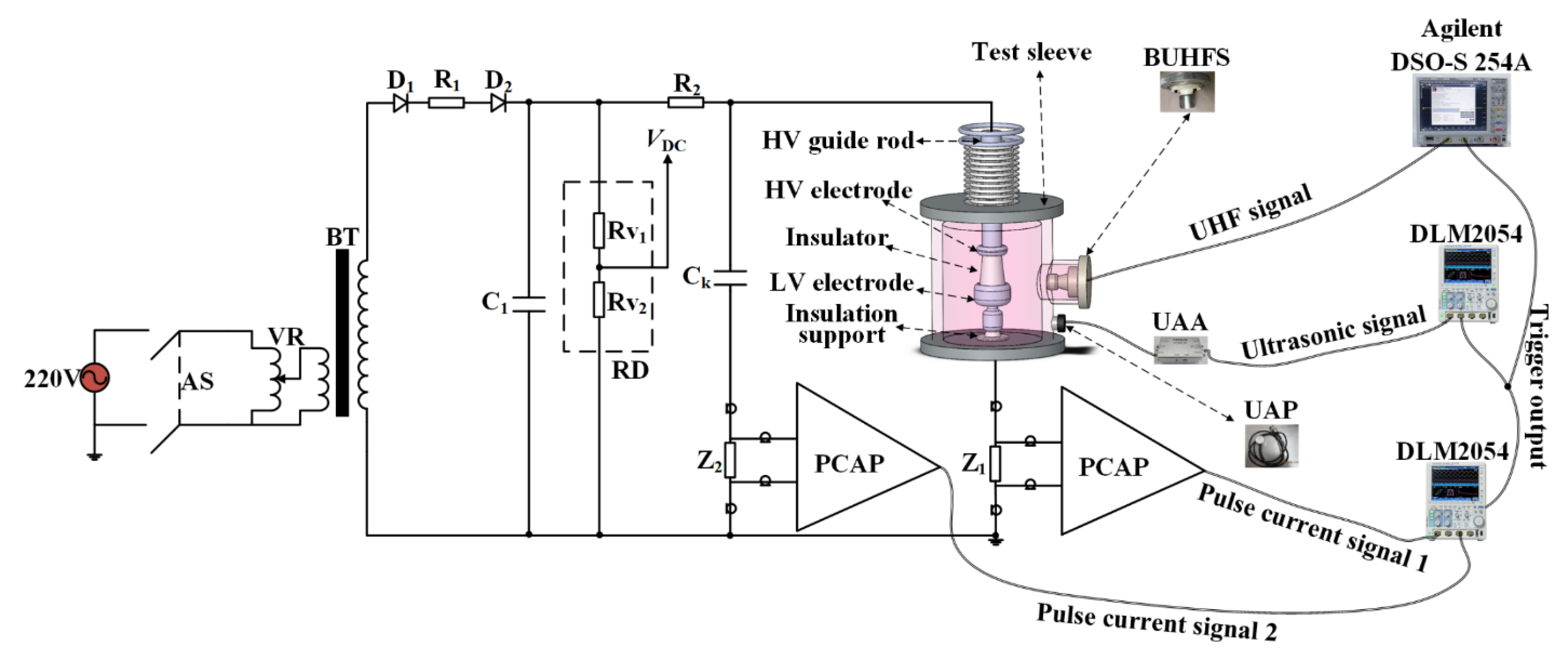
2.1. Experimental Platform

The schematic diagram of the experimental platform is shown in Figure 1, consisting of 220 V AC power supply (powered by WH38905 ultra-isolation transformer), ABB close switch AS, voltage regulator VR, step-up transformer BT (turns ratio is 1:1000), silicon stack D₁ and D₂ (rated rectifier current is 12 mA and rated inverse peak voltage value is 200 kV), protection resistor R₁ (1.6 MΩ), ZWF200-0.1 DC capacitor C₁ (composed of two capacitors 0.1010 μF and 0.1015 μF in series, both of which have a rated voltage of 200 kV), resistor divider (RD, divider ratio is 8000:1), multimeter, protection resistor R₂ (2.13 MΩ), high voltage bushing, test sleeve (mainly consisted of HV electrode, insulator, low-voltage (LV) electrode, and insulation support), SF₆/N₂ gas filling device, signal detection impedance Z₁ and contrast detection impedance Z₂ (Z₁ and Z₂ are both RLC type and identical), coupling capacitor C_k (197.8 pF), pulse current amplifier (PCAP), ultrasonic probe (UAP), ultrasonic amplifier (UAA), built-in UHF sensor (BUHFS), two DLM2054 oscilloscopes (the highest sampling rate is 2.5 GSa/s, and the bandwidth is 500 MHz) and one Agilent DSO-S 254 A oscilloscope (the highest sampling rate is 20 GSa/s, and the bandwidth is 2.6 GHz). Note that only pulse current signals are researched in this paper due to limited space; the other two kinds of signals, UHF signal and ultrasonic signal, will be researched in other papers.

2.2. Insulation Defects

In this paper, four different types of insulation defects are manufactured, corresponding to solid insulation air gap discharge, surface discharge, floating discharge and point discharge, among which the solid insulation air gap defect adopts a self-made vacuum casting block using bisphenol-A epoxy resin shown in Figure 2, and the remaining three types of insulation defects are all set on the GIS post insulator shown in Figure 3. In order to take into account the influences of the defect’s location and size on the pulse current signal, different defect locations or defect sizes are set for the same type of defect. The details are shown as

Table 1. Locations and sizes of four different insulation defects.

Solid Insulation Air Gap Defect				Post Insulator Defects	Surface Defect				Floating Defect			Point Defect
label	1	2	3	label	1	2	3	4	1	2	3	1	2	3
Diameter/mm	2	1	0.5	Diameter/mm	1	0.5	0.5	0.5	0.6	2.5	0.6	0.6	2.5	0.6
Height/mm	2	1	0.5	Length/mm	60	60	30	60	20	20	20	30	30	30
				Distance to HV electrode/mm	10	10	10		1	1		0	0
				Distance to LV electrode/mm				10			1			0

.

3. Statistical Features Extraction from the Inherent Physical Quantities

As stated in Section 1 and Section 2, for each insulation defect, multiple voltage levels were set, ranging from the beginning of stable discharge to the final breakdown or the highest voltage that the experimental platform can provide, and stepwise-boosting voltages were applied with each voltage level lasting for 1 h. Finally, a total of 180,828 pulse current signals were successfully measured, consisting of 540 sample points (one sample point comprises the whole discharge data recorded during the 1 h experiment of the specific insulation defect under the corresponding voltage level, containing at least 50 continuous discharge signals). For each single pulse after being denoised, the corresponding apparent discharge quantity and discharge time, two inherent physical quantities unaffected by the experimental platform and measurement system as well as reflecting the inherent properties of the discharge sources, can be obtained accurately. All the statistical features extracted in this section are based on the above-mentioned two inherent physical quantities.

In general, the extraction of statistical feature quantities is commonly based on the distribution function (continuous case) or probability distribution (discrete case) of one-dimensional or multi-dimensional random variables, which we extend to PD data modes in this paper. PD data modes refer to the statistical relationship diagrams involved with the discharge time, the apparent discharge quantity or their corresponding differences, not necessarily representing probability distributions. The following discussion is focused on a certain discharge sample point.

Assume that the apparent discharge quantity sequence of the current discharge sample point is denoted as Q = {q_r | r = 1, 2, ⋯, SN}, where q_r denotes the apparent discharge quantity of the rth single pulse belonging to the sample point and SN denotes the number of pulses in the current discharge sample point; the discharge time sequence is denoted as PDT = {PDT_r | r = 1, 2, ⋯, SN}, where PDT_r denotes the discharge time of the rth discharge. With regard to the rth discharge, the forward discharge time interval is Δt_pre = PDT_r−PDT_r−1 and the backward discharge time interval is Δt_suc = PDT_r+1 − PDT_r; the first-order difference of apparent discharge quantity is Δq = q_r − q_r−1 and the first-order difference of discharge time interval is Δ(Δt) = PDT_r − 2PDT_r−1 + PDT_r−2. In addition, T denotes the duration of the sample point; n(q_r) and f_PD(q_r) denote the discharge number and discharge repetition rate corresponding to the pluses with apparent discharge quantity equal to q_r; U denotes the DC voltage applied across the insulation defect when obtaining the sample point and U_s denotes the corresponding initial voltage of partial discharge; WP_r (r = 1, 2, ⋯, SN) denotes the energy of the rth discharge and CP denotes the partial discharge cumulative product [34].

As stated above, a PD data mode does not always represent a kind of probability distribution. For a two-dimensional PD data mode, uniformly expressed as y_i = f(x_i), it needs to be first analogized to be the probability distribution of a discrete random variable X. Let all possible values of X be denoted as x₁, x₂, ⋯, x_n (x₁ < x₂ < ⋯< x_n), the corresponding probabilities are p₁, p₂, …, p_n. The transformation formula is shown as Equation (1).

$$p_i=\frac{y_i}{{\displaystyle \sum _{i=1}^n{y}_i}}$$

(1)

By Equation (1), we can calculate the statistical features of any two-dimensional PD data mode (when the PD data mode is a histogram of a certain random variable) or analogical statistical features (when the PD data mode is not a histogram of a certain random variable). The involved features of two-dimensional PD data modes comprise expectation (denoted as m₁), standard deviation (denoted as m₂), skewness (denoted as Skewness), kurtosis (denoted as Kurtosis) and the number of peaks (denoted as Peaks).

When the two-dimensional PD data mode represents a variable histogram, namely the probability distribution (it should be called the frequency distribution to be more precise, an estimate of the actual probability distribution using experimental data), we can use Weibull distribution (when the random variable is non-negative) or one-dimensional kernel density estimation [23] to fit the corresponding probability distribution. Using the maximum likelihood estimation method to fit the Weibull distribution, the corresponding scale parameter α and shape parameter β can be obtained. The kernel density estimation is a non-parametric method of estimating the probability density function. Assuming that the unary probability density function to be estimated is denoted as g, its kernel density estimation function is denoted as $\widehat{g}$ in Equation (2), where K is a non-negative kernel function and h is a smoothing parameter or referred to as bandwidth. We adopt the adaptive kernel density estimator based on the linear diffusion process proposed by [40] to estimate the optimal smoothing parameter h_best.

$$\{\begin{array}{l}\widehat{g}(x|h)=\frac{1}{nh}{\displaystyle \sum _{i=1}^{n}K\left(\frac{x-x_i}{h}\right)}\\ h_{\mathrm{best}}=\underset{h}{\arg \min }\left\{E_f\left[{\displaystyle \int {\left(\widehat{g}(x|h)-g(x)\right)}^2\mathrm{d}x}\right]\right\}\end{array}$$

(2)

Similarly, when the three-dimensional PD data mode represents a binary histogram, namely a two-dimensional probability distribution, two-dimensional kernel density estimation can be used to fit the corresponding probability distribution, and finally, two optimal smoothing parameters can be calculated [40], denoted as H_x and H_y. The energy entropy of the binary histogram can also be calculated by Equation (3), denoted as Entropy, where F_i denotes the probability (frequency to be more precise) corresponding to the (i, j)th binary grid.

$$Entropy=-{\displaystyle \sum _i{\displaystyle \sum _j{F}_i\ln F_i}}$$

(3)

We first introduce each PD data mode used in this paper labelled from A to L, and then detail the extracted statistical features based on the corresponding PD data mode.

A.

H_n(q)

H_n(q) is the frequency density histogram of q. The extracted statistical features consist of m₁, m₂, Skewness, Kurtosis, Peaks, Weibull distribution fitting parameters α and β, as well as the optimal smoothing parameter h_best.

B.

H_n(WP)

H_n(WP) is the frequency density histogram of WP. The extracted statistical features consist of m₁ and m₂.

C.

H_n(Δq)

H_n(Δq) is the frequency density histogram of Δq. The extracted statistical features consist of m₁, m₂, Skewness, Kurtosis, Peaks, and the optimal smoothing parameter h_best.

D.

H_n(ln(Δt))

H_n(ln(Δt)) is the frequency density histogram of ln(Δt). The extracted statistical features consist of m₁, m₂, Skewness, Kurtosis, Peaks, and the optimal smoothing parameter h_best. In addition, the Weibull distribution can be used to fit the probability distribution function of Δt, which must always be non-negative, to obtain the fitting parameters α and β.

E.

Hq(CP)

Hq(CP) is the two-dimensional relationship diagram of PD cumulative product CP [34] calculated by Equation (4) and apparent discharge quantity q. The extracted statistical features consist of m₁, m₂, Skewness, and Kurtosis.

$$\{\begin{array}{l}CP(q)=q\bullet {\displaystyle \sum _{q_r\ge q}{f}_{\mathrm{PD}}(q_r)}=\frac{q\bullet {\displaystyle \sum _{q_r\ge q}n(q_r)}}{T}\\ q\in [\min (Q),\max (Q)]\end{array}$$

(4)

Since the discharge time interval Δt generally does not keep the same, it is necessary to sort all Δt first, and then set an appropriate interval range to divide ln(Δt) at equal intervals in order to make a PD data mode of q and Δt. Let the total number of intervals be NI, q_n (n = 1, 2, ⋯, NI) denote the average of all the apparent discharge quantities in the nth interval and q_max denote the corresponding maximum of all the apparent discharge quantities in the nth interval. Then, we can derive the following four PD data modes, of which the extracted statistical features consist of m₁, m₂, Skewness, Kurtosis and Peaks.

F.

Hq_n(ln(Δt_suc))

Hq_n(ln(Δt_suc)) is the two-dimensional relationship diagram between q_n and ln(Δt_suc).

G.

Hq_max(Δt_suc)

Hq_max(Δt_suc) is the two-dimensional relationship diagram between q_max and ln(Δt_suc).

H.

Hq_n(ln(Δt_pre))

Hq_n(Δt_pre) is the two-dimensional relationship diagram between q_n and ln(Δt_pre).

I.

Hq_max(ln(Δt_pre))

Hq_max(Δt_pre) is the two-dimensional relationship diagram between q_max and ln(Δt_pre).

Analogous to the AC PD phase distribution pattern, describing the difference in the distribution shapes of the two-dimensional relationship diagrams corresponding to the positive and negative half cycle of power frequency period, the above four PD data modes can be used to construct two combination diagrams, one of which combines H_qn(ln(Δt_suc)) with H_qn(ln(Δt_pre)) and the other of which combines H_qmax(ln(Δt_suc)) with H_qmax(ln(Δt_pre)). From the combination diagrams, the extracted statistical features consist of cross-correlation factor and degree of asymmetry, denoted as CC and Asymmetry, respectively. Let y_1i (i = 1,2, ⋯, n) represent the ordinate values of H_qn(Δt_suc) or H_qmax(Δt_suc) and y_2i (i = 1,2, ⋯, n) represent the ordinate values of H_qn(Δt_pre) or H_qmax(Δt_pre); CC and Asymmetry can be calculated as Equation (5).

$$CC=\frac{{\displaystyle \sum _{i=1}^n{y}_{1i}{y}_{2i}}-\frac{1}{n}{\displaystyle \sum _{i=1}^n{y}_{1i}}\bullet {\displaystyle \sum _{i=1}^n{y}_{2i}}}{\sqrt{\left[{\displaystyle \sum _{i=1}^n{y}_{1i}{}^2}-\frac{1}{n}{\left({\displaystyle \sum _{i=1}^n{y}_{1i}}\right)}^2\right]}\bullet \sqrt{\left[{\displaystyle \sum _{i=1}^n{y}_{2i}{}^2}-\frac{1}{n}{\left({\displaystyle \sum _{i=1}^n{y}_{2i}}\right)}^2\right]}},Asymmetry=\frac{{\displaystyle \sum _{i=1}^n{y}_{2i}}}{{\displaystyle \sum _{i=1}^n{y}_{1i}}}$$

(5)

In this paper, binary joint distributions are also used as three-dimensional PD data modes labelled from J to L, which take the apparent discharge quantity q, the discharge time interval Δt or their corresponding differences as the joint variables, of which the extracted statistical features consist of H_x and H_y, two optimal smoothing parameters of two-dimensional kernel density estimation, as well as energy entropy Entropy.

J.

H_n(q, ln(Δt))

H_n(q, ln(Δt)) is a binary histogram of the apparent discharge quantity q and the natural logarithm of discharge time interval ln(Δt), with two cases H_n(q, ln(Δt_suc)) and H_n(q, ln(Δt_pre)), illustrated as Figure 4 and Figure 5, respectively, in which the fitting results of two-dimensional kernel density estimation are also given.

K.

H_n(Δq,ln(Δt))

H_n(Δq, ln(Δt)) is a binary histogram of the first-order difference of apparent discharge quantity Δq and the natural logarithm of discharge time interval ln(Δt), with two cases H_n(Δq, ln(Δt_suc)) and H_n(Δq, ln(Δt_pre)), illustrated as Figure 6 and Figure 7, respectively, in which the fitting results of two-dimensional kernel density estimation are also given.

L.

H_n(Δq, ln|Δ(Δt)|)

H_n(Δq, ln|Δ(Δt)|) is a binary histogram of the first-order difference of apparent discharge quantity Δq and the natural logarithm of the absolute value of the first-order difference of discharge time interval ln|Δ(Δt)|. Considering that Δ(Δt) is not always a positive number, the two cases of Δ(Δt) > 0 and Δ(Δt) < 0 are taken into account separately, illustrated as Figure 8 and Figure 9, respectively, in which the fitting results of two-dimensional kernel density estimation are also given.

4. GDCA and Its Kernelization Forms

This section promotes the supervised subspace projection technology from BDCA to GDCA and its kernelization forms. Some indispensable terminologies and symbols should first be introduced [4,23]:

Recognition Vector: denoted as x_i∈ℝ^M×1 (i = 1, 2, ⋯, N), consists of all statistical features of the ith discharge sample point. The corresponding ones in the intrinsic vector space and the empirical vector space are denoted as $\overrightarrow{\mathit{\varphi }}(x)\in {ℝ}^{J\times 1}$ and $\overrightarrow{k}(x)\in {ℝ}^{N\times 1}$, respectively, where M denotes the number of features, J denotes the dimensionality of the reproducing kernel Hilbert space (i.e., intrinsic vector space) and N denotes the number of samples. According to Section 3, M = 70 and N = 540.

Feature Sample Matrix: denoted as X∈ℝ^M×N, consists of all available recognition vectors.

Class Number: denoted as CN, the total number of all classes. According to Section 2, CN = 4.

Within-class Scatter Matrix: denoted as S_W∈ℝ^M×M.

Between-class Scatter Matrix: denoted as S_B∈ℝ^M×M.

Center-adjusted Scatter Matrix: denoted as S_C∈ℝ^M×M.

Different from the derivation of BDCA [4], the newly proposed GDCA in this paper starts directly from PC-DCA shown in Equation (6) and improves the corresponding constraint condition, which can be more robust and flexible than BDCA. Then, BDCA can be regarded as a special case of the proposed GDCA under a specific parameter value.

$$W_P=\underset{W\in {ℝ}^{M\times m}}{\arg \max }\left\{trace\left[W^{\mathrm{T}}(S_C+\rho I)W\right]|W^{\mathrm{T}}{S}_{W}W=I\right\}$$

(6)

At first, the projection matrix of PC-DCA in Equation (6) is divided into two parts: signal-subspace projection matrix W_PS and noise-subspace projection matrix W_PN. Without loss of generality, suppose that the projected dimensionality m is larger than rank(S_B), and then Equation (6) can be transformed into Equation (7) according to the signal-subspace and the noise-subspace.

$$\{\begin{array}{l}{W}_{PS}=\underset{W\in {ℝ}^{M\times \mathrm{rank}\left(S_B\right)}}{\arg \max }\left\{trace\left[W^{\mathrm{T}}(S_C+\rho I)W\right]|W^{\mathrm{T}}{S}_{W}W=I\right\}\\ W_{PN}=\underset{W\in {ℝ}^{M\times \left[m-\mathrm{rank}\left(S_B\right)\right]}}{\arg \max }\left\{trace\left[W^{\mathrm{T}}(S_C+\rho I)W\right]|W^{\mathrm{T}}{S}_{W}W=I,W^{\mathrm{T}}{S}_{B}W=0\right\}\\ \hspace{1em}\hspace{1em} =\underset{W\in {ℝ}^{M\times \left[m-\mathrm{rank}\left(S_B\right)\right]}}{\arg \max }\left\{trace\left(W^{\mathrm{T}}W\right)|W^{\mathrm{T}}{S}_{W}W=I,W^{\mathrm{T}}{S}_{B}W=0\right\}\end{array}$$

(7)

PC-DCA can be promoted to GDCA by improving the constraint W^TS_WW = I of Equation (7) to W^T(S_W + δI)W = I (δ > ρ, δ → 0⁺ and ρ → 0). Note that signal-subspace projection matrix is also denoted as W_PS and noise-subspace projection matrix is also denoted as W_PN in GDCA, shown as Equation (8):

$$\{\begin{array}{l}{W}_{PS}=\underset{W\in {ℝ}^{M\times \mathrm{rank}\left(S_B\right)}}{\arg \max }\left\{trace\left[W^{\mathrm{T}}(S_C+\rho I)W\right]|W^{\mathrm{T}}(S_W+\delta I)W=I\right\}\\ W_{PN}=\underset{W\in {ℝ}^{M\times \left[m-\mathrm{rank}\left(S_B\right)\right]}}{\arg \max }\left\{trace\left(W^{\mathrm{T}}W\right)|W^{\mathrm{T}}(S_W+\delta I)W=I,W^{\mathrm{T}}{S}_{B}W=0\right\}\\ \hspace{1em}\hspace{1em} =\underset{W\in {ℝ}^{M\times \left[m-\mathrm{rank}\left(S_B\right)\right]}}{\arg \max }\left\{trace\left(\frac{I-W^{\mathrm{T}}{S}_{C}W}{\delta }\right)|W^{\mathrm{T}}(S_W+\delta I)W=I,W^{\mathrm{T}}{S}_{B}W=0\right\}\\ \hspace{1em}\hspace{1em} =\underset{W\in {ℝ}^{M\times \left[m-\mathrm{rank}\left(S_B\right)\right]}}{\arg \min }\left\{trace\left[W^{\mathrm{T}}(S_C+\rho I)W\right]|W^{\mathrm{T}}(S_W+\delta I)W=I,W^{\mathrm{T}}{S}_{B}W=0\right\}\end{array}$$

(8)

It can be seen from Equation (8) that GDCA degenerates into BDCA when ρ = 0. If we temporarily ignore the constraint that W^TS_BW = 0, it can be derived that the discriminant matrix of GDCA is (S_W + δI)⁻¹(S_C + ρI) and the signal-subspace projection matrix W_PS consists of the eigenvectors of (S_W + δI)⁻¹(S_C + ρI) corresponding to the rank(S_B) larger eigenvalues while the noise-subspace projection matrix W_PN consists of the eigenvectors of (S_W + δI)⁻¹(S_C + ρI) corresponding to the m-rank(S_B) smaller eigenvalues. It is only necessary to further prove that W_PN has automatically approximately satisfied the constraint that $W_{PN}^{\mathrm{T}}{S}_B{W}_{PN}=0$ as follows:

Let the m-rank(S_B) smaller eigenvalues of (S_W + δI)⁻¹(S_C + ρI) be arranged in ascending order to form a diagonal matrix Σ_PN, so Equation (9) can be deduced.

$$\begin{array}{l}{(S_W+\delta I)}^{-1}(S_C+\rho I)W_{PN}=W_{PN}{\Sigma }_{PN}\\ \iff {(S_W+\delta I)}^{-1}\left[S_B+(\rho -\delta )I\right]W_{PN}=W_{PN}({\Sigma }_{PN}-I)\\ \iff W_{PN}^{\mathrm{T}}\left[S_B+(\rho -\delta )I\right]W_{PN}=W_{PN}^{\mathrm{T}}(S_W+\delta I)W_{PN}({\Sigma }_{PN}-I)\end{array}$$

(9)

Combining the constraint condition $W_{PN}^{\mathrm{T}}(S_W+\delta I)W_{PN}=I$ in Equations (8) and (9) can be equivalently converted to Equation (10), from which Equation (11) can be further obtained.

$$W_{PN}^{\mathrm{T}}{S}_B{W}_{PN}={\Sigma }_{PN}-I_{[m-\mathrm{rank}(S_B)]\times [m-\mathrm{rank}(S_B)]}+(\delta -\rho )W_{PN}^{\mathrm{T}}{W}_{PN}$$

(10)

$$\{\begin{array}{l}\frac{w_i^{\mathrm{T}}{S}_B{w}_i}{{\Vert w_i\Vert }^2}=\frac{{\lambda }_i-1}{{\Vert w_i\Vert }^2}+\delta -\rho \\ \frac{w_i^{\mathrm{T}}{S}_B{w}_j}{\Vert w_i\Vert \cdot \Vert w_j\Vert }\le \frac{w_i^{\mathrm{T}}{S}_B{w}_j}{\langle w_i,w_j\rangle }=\delta -\rho \\ j\ne i \mathrm{and} i,j=\mathrm{rank}(S_B)+1,\mathrm{rank}(S_B)+2,\cdots ,m\end{array}$$

(11)

Combining Equation (11) with Equation (A11) in the Appendix A and the conclusion that λ_i < 1 (i = rank(S_B) + 1, rank(S_B) + 2, ⋯, m) in the Appendix, Equation (12) can be further derived.

$$\{\begin{array}{l}\frac{w_i^{\mathrm{T}}{S}_B{w}_i}{{\Vert w_i\Vert }^2}=\frac{{\lambda }_i-1}{{\displaystyle \sum _{j=1}^M\frac{1}{{\mu }_j}{u}_{ji}^2}}+\delta -\rho \le \delta {\lambda }_i-\rho <\delta -\rho \\ i=\mathrm{rank}(S_B)+1,\mathrm{rank}(S_B)+2,\cdots ,m\end{array}$$

(12)

Based on the fact that δ > ρ, δ → 0⁺ and ρ → 0, it can be concluded from Equations (11) and (12) that W_PN has indeed automatically approximately satisfied the constraint that $W_{PN}^{\mathrm{T}}{S}_B{W}_{PN}=0$.

The GDCA algorithm can be given as follows:

GDCA algorithm

(0) 

Prepare Essential Parameters

(0.1) 

Choose the projected dimensionality m;

(0.2) 

Choose regularization parameters δ and ρ, which must satisfy the condition that δ > ρ, δ → 0⁺ and ρ → 0 (for simplicity, let ρ = αδ, δ → 0⁺ and α < 1).

(1) 

Calculate the between-class scatter matrix S_B, within-class scatter matrix S_W, and center-adjusted scatter matrix S_C

(1.1) 

Use data preprocessing methods, such as standard normal density (SND) or min-max normalization (MMN), to preprocess the original recognition vectors [41];

(1.2) 

Denote recognition vectors after preprocessing as x_i∈ℝ^M×1 (i = 1, 2, ⋯, N), then calculate S_B, S_W and S_C.

(2) 

Calculate the projection matrix W_GDCA

(2.1) 

If m is not more than rank(S_B), W_GDCA is consisted of the eigenvectors of (S_W + δI)⁻¹(S_C + ρI) corresponding to the rank(S_B) larger eigenvalues arranged in descending order.

(2.2) 

If m is larger than rank(S_B), the signal-subspace projection matrix W_PS is consisted of the eigenvectors of (S_W + δI)⁻¹(S_C + ρI) corresponding to the rank(S_B) larger eigenvalues arranged in descending order while the noise-subspace projection matrix W_PN is consisted of the eigenvectors of (S_W + δI)⁻¹(S_C + ρI) corresponding to the m-rank(S_B) smaller eigenvalues arranged in ascending order. Finally, W_GDCA = [W_PS, W_PN].

(3) 

Normalize projection vectors

Let each column vector of W_GDCA divide its own 2-norm. For any column vector of W_GDCA, multiply itself by −1 if the element with the largest absolute value is negative.

(4) 

Calculate the feature sample matrix after projection $Y_{GDCA}=W_{GDCA}^{\mathrm{T}}X$

(5) 

Whether to change the values of δ and ρ ? Return to 0.2 if yes and go to next step if no.

(6) 

Whether to change m? Return to 0.1 if yes and output W_GDCA and Y_GDCA if no.

We have proved that GDCA algorithm does meet the SNR criterion in the signal-subspace and the noise-power criterion in the noise-subspace, which means SNRs of projected components in the signal-subspace are arranged in descending order while the noise powers of projected components in the noise-subspace are arranged in ascending order; the details of the proof are shown in the Appendix A. Then, we can extend GDCA to the nonlinear case, KGDCA-Intrinsic-Space and KGDCA-Empirical-Space, by means of Gaussian radial basis kernel function (RBF) K(x_i,x_j) = exp(−γ||x_i−x_j||²), γ > 0. Recognition vectors in the original vector space x_i∈ℝ^M×1 are first mapped to the intrinsic or empirical vector space, and then GDCA is used with regard to intrinsic vectors $\overrightarrow{\mathit{\varphi }}(x)\in {ℝ}^{J\times 1}$ or empirical vectors $\overrightarrow{k}(x)\in {ℝ}^{N\times 1}$, respectively.

5. Results and Discussions

In order to demonstrate the advantages of the newly proposed pattern recognition method based on GDCA and its kernelization forms driven SVM, the test strategy of recognition effect based on the combination of Monte-Carlo experimental method and cross-validation is put forward firstly in this section, by which a wealth of estimation indicators for classification results can be calculated. Then, the criterion aimed at finding the optimal (α, δ) value-pair for GDCA and the optimal (γ, α, δ) value-pair for GDCA’s kernelization forms is given, through which it is possible to optimally select the parameters involved in GDCA and its kernelization forms in advance without using the estimation indicators for classification results, greatly shortening the time of pattern recognition and ensuring the optimal recognition effect. Finally, results and discussions are detailed.

5.1. Test Strategy

First, random sampling is performed on the uniform distribution, so that the recognition vectors of all the discharge sample points are equally divided into five disjoint folds, and then 5-fold cross-validation is performed. Furthermore, the estimation indicators of each fold are calculated separately and the results of 5 folds are averaged. The above process can be regarded as one Monte-Carlo experiment. In order to reduce the impact of the randomness of the data set division on the estimation indicators of the final classification result, the above process is repeated 10 times, which means 10 Monte-Carlo experiments are performed. Finally, the results of the 10 Monte-Carlo experiments are averaged. The whole test strategy is shown in Figure 10. The Binary-SVM presented in Figure 10 adopts two-class support vector classification machine based on soft constraints, also referred to as Binary C-SVC [4]. Let x_i (i = 1, 2, ⋯, N) denote the PD recognition vector corresponding to the ith sample point input to Binary-SVM; y_i (i = 1, 2, ⋯, N), only equal to 1 or −1, denotes the class label of the ith sample point. It is worth noting that x_i (i = 1, 2, ⋯, N) can be recognition vectors in the original vector space or after being projected by means of GDCA or its kernelization forms. After solving the corresponding quadratic programming problem, we can obtain the decision function f(x) with regard to any PD recognition vector x.

Since the kernel matrix is a dense matrix in general and may be too large to store, Professor Chih-Jen Lin et al. [42] developed the LIBSVM toolbox, which is widely used for solving classification and regression problems due to its convenience of adjusting parameters, adopting an SMO-type decomposition method [43,44] to solve the quadratic programming problem.

The above-mentioned Binary-SVM is only specified for a two-class situation, and there mainly exist two kinds of methods to extend Binary SVM to Multiclass-SVM, namely one-versus-one scheme and one-versus-all scheme. The one-versus-one scheme needs to train one Binary-SVM for each possible pair of CN classes, which results in CN(CN − 1)/2 Binary-SVMs. The one-versus-all scheme consisted of CN Binary-SVMs, each of which is trained for one class and all the other classes. This paper adopts the one-versus-one scheme. However, basic Binary-SVM can only obtain the decision value of the test sample. In order to obtain posterior class probabilities, we firstly adopt Equation (13) to convert the decision values output by Binary-SVM into the estimated pairwise class probabilities r_ij (i ≠ j and i, j = 1, 2, ⋯, CN), where parameters A and B can be obtained by solving the regularized maximum likelihood problem of maximizing the log-likelihood function in Equation (14), a kind of relative entropy or Kullback–Leibler divergence [45]. In Equation (14), t_i denotes the maximum a posteriori (MAP) estimation for the target probability shown as Equation (15), consisted of two values, namely t₊ and t₋, corresponding to positive and negative samples, respectively. Compared with t₊ = 1 and t₋ = 0, Equation (15) can effectively avoid the overfitting of Equation (13).

$$r_{ij}=\frac{1}{1+{\mathrm{e}}^{Af+B}}, i\ne j \mathrm{and} i,j=1, 2, \cdots ,CN$$

(13)

$$\underset{A,B}{\max }\left\{{\displaystyle \sum _i\left[t_i\ln r_{ij}+(1-t_i)\ln (1-r_{ij})\right]}\right\}$$

(14)

$$t_i=\{\begin{array}{l}{t}_{+}=\frac{N_{+}+1}{N_{+}+2}, y_i=1\\ t_{-}=\frac{1}{N_{-}+2}, y_i=-1\end{array}$$

(15)

In addition, in order to ensure the unbiasedness of the decision values used to estimate the parameters A and B, all the decision values in Equation (13) are obtained through 5-fold cross-validation of the training data set, which means the decision function is firstly obtained with 4-fold samples, then the decision values of the remaining 1-fold samples are calculated, and we repeat the above process until each training sample has a decision value. For the sample x_t to be classified, we should firstly obtain its estimated pairwise class probabilities r_ij (i ≠ j and i, j = 1, 2, ⋯, CN), then the optimization problem based on the pairwise coupling method in Equation (16) [46] is solved to obtain the final class probabilities $p_t^k=\mathrm{P}(y_t=k|x_t)$(k = 1, 2, ⋯, CN) of Multiclass-SVM. Finally, according to the maximum posterior probability criterion, the class that maximizes $p_t^k$ is used as the predicted class of the test sample. The above pattern recognition can achieve the Bayes optimal decision under the condition of equal cost.

$$\begin{array}{l}\underset{p_t}{\min }{\displaystyle \sum _{i=1}^{CN}{\displaystyle \sum _{j=1,j\ne i}^{CN}{\left(r_{ji}{p}_t^i-r_{ij}{p}_t^j\right)}^2}}\\ \mathrm{subject} \mathrm{to} \mathrm{the} \mathrm{constraints}:\\ {\displaystyle \sum _{k=1}^{CN}{p}_t^k}=1 \mathrm{and} \forall k, p_t^k\ge 0\end{array}$$

(16)

It can be seen from Figure 10 that there exist ten estimation indicators to evaluate the recognition results [41,47]. By extending two-class estimation indicators of pattern recognition to the multi-class situation using class ratio as weight, we can obtain each 1-fold estimation indicator. Then, each 5-fold estimation indicator can be obtained by averaging the corresponding results of all folds.

5.2. Criterion for Selecting Optimal Parameters of GDCA and Its Kernelization Forms

In the actual application of GDCA or its kernelization forms, the optimal (α, δ) or (γ, α, δ) value pair should be determined according to a certain criterion in order to establish the final pattern recognition algorithm, which also shown in Figure 10. In this section, we establish a criterion criterionf_m as shown in Equation (17), which integrates the three technical indicators, namely SNR_i (i = 1, 2, ⋯, rank(S_B)), OSNR_m and WOSNR_m 4. In Equation (17), h_i (i = 1, 2, 3) denote the weights, and N_a, N_b and N_c denote the number of calculated values of γ, α and δ, respectively.

$$\{\begin{array}{l}({\gamma }_{\mathrm{opt}}, {\alpha }_{\mathrm{opt}}, {\delta }_{\mathrm{opt}})=\arg \underset{({\gamma }_a, {\alpha }_b, {\delta }_c)}{\max }\left\{criterion{f}_m({\gamma }_a, {\alpha }_b, {\delta }_c)={\displaystyle \sum _{i=1}^3{h}_i\bullet TI{N}_i}\right\}\\ TI{N}_1=\frac{N_a{N}_b{N}_c{\displaystyle \sum _{i=1}^{\mathrm{rank}(S_B)}SN{R}_i\left({\gamma }_a, {\alpha }_b, {\delta }_c\right)}-{\displaystyle \sum _a{\displaystyle \sum _b{\displaystyle \sum _c{\displaystyle \sum _{i=1}^{\mathrm{rank}(S_B)}SN{R}_i\left({\gamma }_a, {\alpha }_b, {\delta }_c\right)}}}}}{\sqrt{N_a{N}_b{N}_c{\displaystyle \sum _a{\displaystyle \sum _b{\displaystyle \sum _c{\left[{\displaystyle \sum _{i=1}^{\mathrm{rank}(S_B)}SN{R}_i\left({\gamma }_a, {\alpha }_b, {\delta }_c\right)}\right]}^2}}}-{\left[{\displaystyle \sum _a{\displaystyle \sum _b{\displaystyle \sum _c{\displaystyle \sum _{i=1}^{\mathrm{rank}(S_B)}SN{R}_i\left({\gamma }_a, {\alpha }_b, {\delta }_c\right)}}}}\right]}^2}}\\ TI{N}_2=\frac{N_a{N}_b{N}_c·OSN{R}_m\left({\gamma }_a, {\alpha }_b, {\delta }_c\right)-{\displaystyle \sum _a{\displaystyle \sum _b{\displaystyle \sum _{c}OSN{R}_m\left({\gamma }_a, {\alpha }_b, {\delta }_c\right)}}}}{\sqrt{N_a{N}_b{N}_c{\displaystyle \sum _a{\displaystyle \sum _b{\displaystyle \sum _c{\left[OSN{R}_m\left({\gamma }_a, {\alpha }_b, {\delta }_c\right)\right]}^2}}}-{\left[{\displaystyle \sum _a{\displaystyle \sum _b{\displaystyle \sum _{c}OSN{R}_m\left({\gamma }_a, {\alpha }_b, {\delta }_c\right)}}}\right]}^2}}\\ TI{N}_3=\frac{N_a{N}_b{N}_c·WOSN{R}_m\left({\gamma }_a, {\alpha }_b, {\delta }_c\right)-{\displaystyle \sum _a{\displaystyle \sum _b{\displaystyle \sum _{c}WOSN{R}_m\left({\gamma }_a, {\alpha }_b, {\delta }_c\right)}}}}{\sqrt{N_a{N}_b{N}_c{\displaystyle \sum _a{\displaystyle \sum _b{\displaystyle \sum _c{\left[WOSN{R}_m\left({\gamma }_a, {\alpha }_b, {\delta }_c\right)\right]}^2}}}-{\left[{\displaystyle \sum _a{\displaystyle \sum _b{\displaystyle \sum _{c}WOSN{R}_m\left({\gamma }_a, {\alpha }_b, {\delta }_c\right)}}}\right]}^2}}\end{array}$$

(17)

5.3. Recognition Effects of GDCA and Its Kernelization Forms Driven SVM

This section gives the recognition effects of GDCA and its kernelization forms driven SVM. Many comparisons are performed, together with the effects of different values of regularization coefficient α on GDCA and its kernelization forms driven SVM researched.

5.3.1. Recognition Effect of GDCA Driven SVM

According to the flowchart shown in Figure 10, the estimation indicators of all the Monte-Carlo experiments of GDCA driven SVM and original SVM are calculated, and then we obtain the mean of each estimation indicator by averaging 10 Monte-Carlo experiments, which are denoted as MACA, MASensitivity, MASpecificity, MAPPV, MANPV, MAFmeasure, MAMSE, MAMLL, MAOMCC and MAWMCC. The mean and standard deviation of each estimation indicator of all the Monte-Carlo experiments as well as the sign of the difference between GDCA driven SVM (with MMN preprocessing) and original SVM for the mean of each estimation indicator are shown in Figure 11 (only the results of MACA and MAMLL are displayed due to limited space). Results show that there exist values of δ, with which GDCA driven SVM outperforms original SVM with regard to all the estimation indicators except MASpecificity under all the values of α. All the standard deviations of 10 Monte-Carlo experiments for each estimation indicator by GDCA driven SVM are less than those by original SVM, which means GDCA driven SVM is more robust than original SVM. In addition, by maximizing criterionf₁₀ established in Section 5.2, it is derived that α_opt = 0.9, δ_opt = 10⁻⁴, under which MACA can arrive at the maximum of 92.41%. The consuming time of executing all the Monte-Carlo experiments by GDCA driven SVM has the mean of 403.9399 s and the standard deviation of 53.3158 s, while the time consumed by original SVM is 1697.9388 s. The above time is counted using MATLAB on a personal computer with 2.50 GHz CPU and 16.0 GB RAM.

The increased percentage and the sign of estimation indicators comparing GDCA driven SVM with BDCA driven SVM under different values of α are shown in Figure 12 (only display the case of α = 0.5 due to limited space). Results show that the range of δ, in which GDCA outperforms BDCA with regard to all the estimation indicators, generally expands as α expands. Especially, GDCA (0 < α < 1) is superior to BDCA in the majority span of δ.

5.3.2. Recognition Effect of GDCA’s Kernelization Forms Driven SVM

According to the flowchart shown in Figure 10, the estimation indicators of all the Monte-Carlo experiments by KGDCA-Intrinsic-Space- and KGDCA-Empirical-Space driven SVM under different values of γ, α and δ are calculated. The consuming time of executing all the Monte-Carlo experiments by KGDCA-Intrinsic-Space/KGDCA-Empirical-Space driven SVM has means of 515.5661 s/468.8253 s and standard deviations of 241.1514 s/276.1790 s, respectively.

●

Comparisons between KGDCA-Intrinsic-Space/KGDCA-Empirical-Space driven SVM and original SVM

Comparisons of the mean of each estimation indicator by averaging all the 10 Monte-Carlo experiments between KGDCA-Intrinsic-Space/KGDCA-Empirical-Space driven SVM and original SVM under different values of α are shown in Figure 13 (only the cases under α = 0.9 are displayed due to limited space). The results show that there exist large numbers of combinations of (γ, α, δ), by which KGDCA-Intrinsic-Space/KGDCA-Empirical-Space driven SVM is superior to original SVM. In addition, the range of γ, in which KGDCA-Intrinsic-Space/KGDCA-Empirical-Space outperforms original SVM, generally expands as δ decreases. In addition, by maximizing criterionf₁₀ established in Section 5.2, it is derived that γ_opt = 2⁻³, α_opt = 0.9, δ_opt = 10⁻⁵ for KGDCA-Intrinsic-Space driven SVM, under which MACA can arrive at the maximum of 100%, meaning the results that all the test samples of all the Monte-Carlo experiments have been classified successfully and γ_opt = 2⁻¹, α_opt = 0.9, δ_opt = 10⁻⁶ for KGDCA-Empirical-Space driven SVM, under which MACA can arrive at 99.83%.

●

Comparisons between KGDCA-Intrinsic-Space/KGDCA-Empirical-Space driven SVM and GDCA driven SVM

The increased percentages of all the estimation indicators comparing KGDCA-Intrinsic-Space/KGDCA-Empirical-Space driven SVM with GDCA driven SVM under different values of γ, α and δ are shown in Figure 14 (only the case under α = 0.9 for MACA is displayed due to limited space). The results show that in the overwhelmingly major combinations of γ and δ under all the values of α, KGDCA-Intrinsic-Space/KGDCA-Empirical-Space driven SVM outperforms GDCA driven SVM. The maximum increased ratios with regard to MACA, MASensitivity, MASpecificity, MAPPV, MANPV, MAFmeasure, MAMSE, MAMLL, MAOMCC and MAWMCC for KGDCA-Intrinsic-Space driven SVM are 15.53%, 15.53%, 5.48%, 15.19%, 4.86%, 15.82%, 99.79%, 94.95%, 21.84% and 22.40%, respectively, while the corresponding ones for KGDCA-Empirical-Space driven SVM are 15.53%, 15.53%, 5.48%, 15.19%, 4.86%, 15.82%, 99.78%, 95.24%, 21.84% and 22.40%, respectively.

●

Effect of α on KGDCA-Intrinsic-Space/KGDCA-Empirical-Space driven SVM

The relationships describing the sign of the difference of all the estimation indicators between KGDCA-Intrinsic-Space/KGDCA-Empirical-Space (0 < α < 1) and KGDCA-Intrinsic-Space/KGDCA-Empirical-Space (α = 0) driven SVM varying with the values of γ and δ are shown as Figure 15 (only the case under α = 0.9 for MACA is displayed due to limited space). The results show that KGDCA-Intrinsic-Space/KGDCA-Empirical-Space (0 < α < 1) driven SVM outperforms KGDCA-Intrinsic-Space/KGDCA-Empirical-Space (α = 0) driven SVM in the overwhelmingly major combinations of γ and δ except the range in which they are tied.

5.4. Comparisons with Other Dimensionality Reduction Algorithms

In this section, we use the test strategy in Section 5.1 to compare the newly proposed method with 36 kinds of state-of-the-art dimensionality reduction algorithms. Although we calculate 10 estimation indicators to evaluate the recognition results, only results of MACA are shown in Figure 16 due to limited space. It can be seen from the results that the proposed method outperforms all the compared feature selection ones, comprising filter type, wrapper type and embedded type, since the proposed method uses all the information contained in the recognition vectors but feature selection methods inevitably discard some useful information. In the meantime, the wrapper type and embedded type are always classifier-dependent and not only computationally intensive but also at risk of overfitting. In addition, the proposed method also outperforms all the compared unsupervised subspace projection ones, which can be attributed to the fact that the unsupervised subspace projection technology does not involve any class information. Even compared with supervised subspace projection technologies, our proposed method still demonstrates competitive performances with significant advantages.

5.5. Comparisons with Other Classifiers

In this section, we use the test strategy in Section 5.1 to compare the newly proposed method with other state-of-the-art classifiers adopted in mainstream pattern recognition methods, composed of ten kinds of neural networks [48], classical rough set (CRS) [49], neighborhood classifier (NEC) [50], K nearest neighbor classifier (KNN), classification and regression tree (CART), C4.5, Naive Bayes classifier (NBC), linear discriminant analysis (LDA), quadratic discriminant analysis (QDA), kernelized discriminant analysis (KDA) [4] and ensemble algorithms (including bootstrap aggregating and random subspace ensembles) [51], as well as their combinations with feature selection (also referred to as attribute reduction) using neighborhood rough set (NRS) [50]. All the involved parameters in the above methods are chosen according to 5-fold cross validation.

5.5.1. Comparisons with Ten Kinds of Neural Networks

Ten representative kinds of neural networks, comprising convolutional neural network (CNN), adaptive neuro-fuzzy inference system (ANFIS), back-propagation neural network (BPNN), Hopfield neural network (HNN), radial basis function neural network (RBFNN), generalized regression neural network (GRNN), wavelet neural network (including two cases of Morlet wavelet and Mexican hat wavelet, referred to as WNNMo and WNNMe, respectively), learning vector quantization neural network (LVQNN), counter propagation neural network (CPNN) and probabilistic neural network (PNN), were chosen to make comparisons with the newly proposed pattern method. The results of the mean and standard deviation of all the Monte-Carlo experiments for ACA are shown in Figure 17a, from which it can be seen that both GDCA driven SVM and GDCA’s kernelization forms driven SVM are superior to the chosen neural networks.

5.5.2. Comparisons with CRS

CRS is specified for discrete features, so it is indispensable to carry out proper discretization of continuous features before using CRS. Eight discretization methods were chosen, comprising four unsupervised algorithms based on hierarchical clustering (HRC), K-means, Gaussian mixing model (GMM) [48], fuzzy C-means clustering (FCM) [52], together with four supervised algorithms based on ChiMerge, information entropy (IFE), class-attribute contingency coefficient (CACC) and class-attribute interdependence maximization (CAIM) [53], the corresponding results of which are shown in Figure 17b, from which it can be seen that both GDCA driven SVM and GDCA’s kernelization forms driven SVM are superior to CRS with all the eight discretization methods.

5.5.3. Comparisons with the Remaining Classifiers

●

Without attribute reduction of NRS

The results of the remaining recognition methods, namely NEC, CART, KNN, C4.5, NBC (considering two cases of normal probability density estimation and kernel density estimation, referred to as NBCN and NBCK, respectively), LDA, QDA, KDA, bootstrap aggregating of CART (BACART) and random subspace ensembles of KNN, LDA and QDA (referred to as RSKNN, RSLDA and RSQDA, respectively), without attribute reduction of NRS, are shown in Figure 17c.

●

with attribute reduction of NRS

The results of the remaining recognition methods, namely NEC, CART, KNN, C4.5, NBCN, NBCK, LDA, QDA, KDA, BACART, RSKNN, RSLDA and RSQDA, with attribute reduction of NRS, are shown in Figure 17d.

6. Conclusions

By building a set of 220 kV HVDC GIS experiment platform and manufacturing four different types of insulation defects (including multiple sizes and positions), we successfully measured 180,828 pulse current signals under multiple voltage levels. After being denoised, the apparent discharge quantity and the discharge time, two inherent physical quantities unaffected by the experimental platform and measurement system, were obtained, according to which 70 statistical features were extracted. We detailed a pattern recognition method based on generalized discriminant component analysis and its kernelized forms driven SVM, and established the corresponding selection criterion of involved parameters. Combining the Monte-Carlo experimental method with the cross-validation test strategy, 10 evaluation indicators for classification results were calculated. Then, recognition effects of GDCA and its kernelization forms driven SVM including comparisons between each other were analyzed in detail. Finally, comparisons between the newly proposed pattern recognition method and 36 kinds of state-of-the-art dimensionality reduction algorithms together with 44 kinds of state-of-the-art classifiers were performed. The following conclusions can be drawn:

(1)

All the problems of BDCA mentioned in Section 1 can be resolved by GDCA as well as its kernelization forms proposed in this paper. The range of δ, in which GDCA outperforms BDCA with regard to all the estimation indicators, generally expands as α expands. Especially, GDCA (0 < α < 1) is superior to BDCA in the majority span of δ. In the overwhelmingly major combinations of γ and δ under all the values of α, KGDCA-Intrinsic-Space/KGDCA-Empirical-Space outperformed GDCA.

(2)

By establishing an effective criterion to optimally select the parameters involved in GDCA and its kernelization forms in advance without using the evaluation indicators of classification results, the time of pattern recognition can be shortened considerably to ensure the optimal recognition effect simultaneously.

(3)

The newly proposed pattern recognition method greatly improved the recognition accuracy in comparison with 36 kinds of state-of-the-art dimensionality reduction algorithms and 44 kinds of state-of-the-art classifiers.

Due to the fact that only the apparent discharge quantity and the discharge time, two inherent physical quantities unaffected by the experimental platform and measurement system, are needed, this newly proposed method not only solves the difficulty that phase-resolved partial discharge (PRPD) cannot be applied under DC conditions, but also immensely facilitates the fault diagnosis of HVDC GIS.

References

1. Wenger, P.; Beltle, M.; Tenbohlen, S.; Riechert, U.; Behrmann, G. Combined characterization of free-moving particles in HVDC-GIS using UHF PD, high-speed imaging, and pulse-sequence analysis. IEEE Trans. Power Deliv. 2019, 34, 1540–1548. [Google Scholar] [CrossRef]
2. Magier, T.; Tenzer, M.; Koch, H. Direct current gas-insulated transmission lines. IEEE Trans. Power Deliv. 2018, 33, 440–446. [Google Scholar] [CrossRef]
3. Ridder, D.D.; Tax, D.M.J.; Lei, B.; Xu, G.; Feng, M.; Zou, Y.; van der Heijden, F. Classification, Parameter Estimation and State Estimation: An Engineering Approach Using MATLAB, 2nd ed.; John Wiley & Sons: Hoboken, NJ, USA, 2017. [Google Scholar]
4. Kung, S.Y. Kernel Methods and Machine Learning; Cambridge University Press: Cambridge, UK, 2014. [Google Scholar]
5. Hira, Z.M.; Gillies, D.F. A review of feature selection and feature extraction methods applied on microarray data. Adv. Bioinform. 2015, 2015, 198363. [Google Scholar] [CrossRef]
6. Kis, K.B.; Fodor, Á.; Büki, M.I. Adaptive, Hybrid Feature Selection (AHFS). Pattern Recognit. 2021, 116, 107932. [Google Scholar]
7. Yun, L.; Tao, L.; Liu, H. Recent advances in feature selection and its applications. Knowl. Inf. Syst. 2017, 53, 551–577. [Google Scholar]
8. Liu, J.; Lin, Y.; Lin, M.; Wu, S.; Zhang, J. Feature selection based on quality of information. Neurocomputing 2017, 225, 11–22. [Google Scholar] [CrossRef]
9. Meenachi, L.; Ramakrishnan, S. Metaheuristic Search Based Feature Selection Methods for Classification of Cancer. Pattern Recognit. 2021, 119, 108079. [Google Scholar] [CrossRef]
10. Zini, L.; Noceti, N.; Fusco, G.; Odone, F. Structured multi-class feature selection with an application to face recognition. Pattern Recognit. Lett. 2015, 55, 35–41. [Google Scholar] [CrossRef]
11. Cawley, G.C.; Talbot, N.L.C. Gene selection in cancer classification using sparse logistic regression with Bayesian regularization. Bioinformatics 2006, 22, 2348–2355. [Google Scholar] [CrossRef] [Green Version]
12. Bernhard, S.; John, P.; Thomas, H. Sparse Multinomial Logistic Regression via Bayesian L1 Regularization. Adv. Neural Inf. Process. Syst. 2017, 19, 209–216. [Google Scholar]
13. Zhang, J.; Luo, Z.; Li, C.; Zhou, C.; Li, S. Manifold regularized discriminative feature selection for multi-label learning. Pattern Recognit. 2019, 95, 136–150. [Google Scholar] [CrossRef]
14. Su, B.; Ding, X.; Wang, H.; Wu, Y. Discriminative dimensionality reduction for multi-dimensional sequences. IEEE Trans. Pattern Anal. Mach. Intell. 2018, 40, 77–91. [Google Scholar] [CrossRef] [PubMed]
15. Yang, J.; Frangi, A.F.; Yang, J.Y.; Zhang, D.; Jin, Z. KPCA plus LDA: A complete kernel Fisher discriminant framework for feature extraction and recognition. IEEE Trans. Pattern Anal. Mach. Intell. 2005, 27, 230–244. [Google Scholar] [CrossRef] [PubMed] [Green Version]
16. Tipping, M.; Bishop, C. Probabilistic principal component analysis. J. R. Stat. Soc. 1999, 61, 611–622. [Google Scholar] [CrossRef]
17. Kruskal, J.B. Multidimensional scaling by optimizing goodness of fit to a nonmetric hypothesis. Psychometrika 1964, 29, 230–244. [Google Scholar] [CrossRef]
18. Wu, M.; Cao, H.; Cao, J.; Nguyen, H.L.; Gomes, J.B.; Krishnaswamy, S.P. An overview of state-of-the-art partial discharge analysis techniques for condition monitoring. IEEE Electr. Insul. Mag. 2015, 31, 22–35. [Google Scholar] [CrossRef]
19. Roweis, S.T.; Saul, L.K. Nonlinear dimensionality reduction by locally linear embedding. Science 2000, 290, 2323–2326. [Google Scholar] [CrossRef] [Green Version]
20. Tenenbaum, J.B.; de Silva, V.; Langford, J.C. A global geometric framework for nonlinear dimensionality reduction. Science 2000, 290, 2319–2323. [Google Scholar] [CrossRef]
21. Sundaresan, A.; Chellappa, R. Model Driven Segmentation of Articulating Humans in Laplacian Eigenspace. IEEE Trans. Pattern Anal. Mach. Intell. 2008, 30, 1771–1785. [Google Scholar] [CrossRef]
22. Li, Y.; Chai, Y.; Zhou, H.; Yin, H. A novel dimension reduction and dictionary learning framework for high-dimensional data classification. Pattern Recognit. 2021, 112, 107793. [Google Scholar] [CrossRef]
23. Duda, R.O.; Hart, P.E.; Stork, D.G. Pattern Classification, 2nd ed.; Wiley-Interscience: Hoboken, NJ, USA, 2001. [Google Scholar]
24. Goldberger, J.; Hinton, G.; Roweis, S.; Salakhutdinov, R. Neighborhood Components Analysis. Adv. Neural Inf. Process. Syst. 2005, 17, 513–520. [Google Scholar]
25. Masoudimansour, W.; Bouguila, N. Supervised dimensionality reduction of proportional data using mixture estimation. Pattern Recognit. 2020, 105, 107379. [Google Scholar] [CrossRef]
26. Bian, W.; Tao, D. Asymptotic Generalization Bound of Fisher’s Linear Discriminant Analysis. IEEE Trans. Pattern Anal. Mach. Intell. 2014, 36, 2325–2337. [Google Scholar] [CrossRef] [PubMed]
27. Yu, Y.; McKelvey, T.; Kung, S.Y. A classification scheme for ‘high-dimensional-small-sample-size’ data using soda and ridge-SVM with microwave measurement applications. In Proceedings of the IEEE International Conference on Acoustics, Speech and Signal Processing, Vancouver, BC, Canada, 36–31 May 2013; pp. 3542–3546. [Google Scholar]
28. Rahulamathavan, Y.; Phan, R.C.; Chambers, J.A.; Parish, D.J. Facial Expression Recognition in the Encrypted Domain Based on Local Fisher Discriminant Analysis. IEEE Trans. Affect. Comput. 2013, 4, 83–92. [Google Scholar] [CrossRef]
29. Lai, Z.; Xu, Y.; Yang, J.; Shen, L.; Zhang, D. Rotational invariant dimensionality reduction algorithms. IEEE Trans. Cybern. 2016, 47, 3733–3746. [Google Scholar] [CrossRef]
30. Zhang, X.; Chu, D.; Tan, R.C. Sparse uncorrelated linear discriminant analysis for undersampled problems. IEEE Trans. Neural Netw. Learn. Syst. 2016, 27, 1469–1485. [Google Scholar] [CrossRef]
31. Zhao, H.; Wang, Z.; Nie, F. A new formulation of linear discriminant analysis for robust dimensionality reduction. IEEE Trans. Knowl. Data Eng. 2018, 31, 629–640. [Google Scholar] [CrossRef]
32. Zhang, D.; Li, X.; He, J.; Du, M. A new linear discriminant analysis algorithm based on L1-norm maximization and locality preserving projection. Pattern Anal. Appl. 2018, 21, 685–701. [Google Scholar] [CrossRef]
33. Peng, X.; Yang, F.; Wang, G.; Wu, Y.; Li, L.; Li, Z.; Bhatti, A.A.; Zhou, C.; Hepburn, D.M.; Reid, A.J.; et al. A convolutional neural network based deep learning methodology for recognition of partial discharge patterns from high voltage cables. IEEE Trans. Power Deliv. 2019, 34, 1460–1469. [Google Scholar] [CrossRef]
34. Morshuis, P.H.F.; Smit, J.J. Partial discharges at DC voltage: Their mechanism, detection and analysis. IEEE Trans. Dielectr. Electr. Insul. 2005, 12, 328–340. [Google Scholar] [CrossRef] [Green Version]
35. Seo, I.J.; Khan, U.A.; Hwang, J.S.; Lee, J.G.; Koo, J.Y. Identification of insulation defects based on chaotic analysis of partial discharge in HVDC superconducting cable. IEEE Trans. Appl. Supercond. 2015, 25, 1–5. [Google Scholar] [CrossRef]
36. Pirker, A.; Schichler, U. Partial discharges at DC voltage - measurement and pattern recognition. In Proceedings of the IEEE International Conference on Condition Monitoring and Diagnosis, Xi’an, China, 25–28 September 2016. [Google Scholar]
37. Yang, F.; Sheng, G.; Xu, Y.; Hou, H.; Qian, Y.; Jiang, X. Partial discharge pattern recognition of XLPE cables at DC voltage based on the compressed sensing theory. IEEE Trans. Dielectr. Electr. Insul. 2017, 24, 2977–2985. [Google Scholar] [CrossRef]
38. Wenrong, S.; Junhao, L.; Peng, Y.; Yanming, L. Digital detection, grouping and classification of partial discharge signals at DC voltage. IEEE Trans. Dielectr. Electr. Insul. 2008, 15, 1663–1674. [Google Scholar] [CrossRef]
39. Varol, Y.; Oztop, H.F.; Avci, E. Estimation of thermal and flow fields due to natural convection using support vector machines (SVM) in a porous cavity with discrete heat sources. Int. Commun. Heat Mass Transf. 2008, 35, 928–936. [Google Scholar] [CrossRef]
40. Botev, Z.I.; Grotowski, J.F.; Kroese, D.P. Kernel density estimation via diffusion. Ann. Stat. 2010, 38, 2916–2957. [Google Scholar] [CrossRef] [Green Version]
41. Umbaugh, S.E. Digital Image Processing and Analysis: Applications with MATLAB and CVIPtools, 3rd ed.; CRC Press: Boca Raton, FL, USA, 2018. [Google Scholar]
42. Chang, C.C.; Lin, C.J. LIBSVM: A library for support vector machines. ACM Trans. Intell. Syst. Technol. 2011, 2, 1–27. [Google Scholar] [CrossRef]
43. Fan, R.E.; Chen, P.H.; Lin, C.J.; Joachims, T. Working set selection using second order information for training support vector machines. J. Mach. Learn. Res. 2005, 6, 1889–1918. [Google Scholar]
44. Chen, P.H.; Fan, R.E.; Lin, C.J. A study on SMO-type decomposition methods for support vector machines. IEEE Trans. Neural Netw. 2006, 17, 893–908. [Google Scholar] [CrossRef] [PubMed] [Green Version]
45. Platt, J.C. Probabilistic outputs for support vector machines and comparisons to regularized likelihood methods. Adv. Large Margin Classif. 2000, 10, 61–74. [Google Scholar]
46. Wu, T.F.; Lin, C.J.; Weng, R.C. Probability estimates for multi-class classification by pairwise coupling. J. Mach. Learn. Res. 2004, 5, 975–1005. [Google Scholar]
47. Mak, M.W.; Guo, J.; Kung, S.Y. PairProSVM: Protein subcellular localization based on local pairwise profile alignment and SVM. IEEE/ACM Trans. Comput. Biol. Bioinform. 2008, 5, 416–422. [Google Scholar] [PubMed]
48. Brunton, S.L.; Kutz, J.N. Data-Driven Science and Engineering: Machine Learning, Dynamical Systems, and Control; Cambridge University Press: Cambridge, UK, 2019. [Google Scholar]
49. Pawlak, Z. Rough sets. Int. J. Parallel Program. 1982, 11, 341–356. [Google Scholar] [CrossRef]
50. Hu, Q.H.; Yu, D.R.; Xie, Z.X. Neighborhood classifiers. Expert Syst. Appl. 2008, 34, 866–876. [Google Scholar] [CrossRef]
51. Zhou, Z.H. Ensemble Methods Foundations and Algorithms; CRC Press: Boca Raton, FL, USA, 2012. [Google Scholar]
52. Li, Y.; Gou, J.; Fan, Z.W. Educational data mining for students’ performance based on fuzzy C-means clustering. IET Gener. Transm. Distrib. 2019, 2019, 8245–8250. [Google Scholar] [CrossRef]
53. Garcia, S.; Luengo, J.; Sáez, J.A.; Lopez, V.; Herrera, F. A Survey of Discretization Techniques: Taxonomy and Empirical Analysis in Supervised Learning. IEEE Trans. Knowl. Data Eng. 2013, 25, 734–750. [Google Scholar] [CrossRef]
Figure 1. The schematic diagram of the experimental platform.
Energies 14 07674 g001
Figure 2. The schematic diagram of solid insulation air gap defect.
Energies 14 07674 g002
Figure 3. The dimensioning of insulator and the schematic diagrams of No. 4 surface defect, No. 2 floating defect and No. 3 point defect. (a) Dimensioning of insulator; (b) No. 4 surface defect; (c) No. 2 floating defect; (d) No. 3 point defect.
Energies 14 07674 g003
Figure 4. The illustration of Hn(q, ln(Δtsuc)) and the corresponding result of two−dimensional kernel density estimation.
Energies 14 07674 g004
Figure 5. The illustration of Hn(q, ln(Δtpre)) and the corresponding result of two−dimensional kernel density estimation.
Energies 14 07674 g005
Figure 6. The illustration of Hnq, ln(Δtsuc)) and the corresponding result of two−dimensional kernel density estimation.
Energies 14 07674 g006
Figure 7. The illustration of Hnq, ln(Δtpre)) and the corresponding result of two−dimensional kernel density estimation.
Energies 14 07674 g007
Figure 8. The illustration of Hnq, ln|Δ(Δt)|) and the corresponding result of two−dimensional kernel density estimation when Δ(Δt) > 0.
Energies 14 07674 g008
Figure 9. The illustration of Hnq, ln|Δ(Δt)|) and the corresponding result of two−dimensional kernel density estimation when Δ(Δt) < 0.
Energies 14 07674 g009
Figure 10. Test strategy of the newly proposed pattern recognition by combining Monte-Carlo experiment with cross-validation.
Energies 14 07674 g010
Figure 11. Comparisons between GDCA driven SVM and original SVM regarding the mean and standard deviation of all the Monte−Carlo experiments for ACA and AMLL. (a) The mean of ACA (MACA). (b) The sign of the difference of MACA. (c) The standard deviation of ACA. (d) The mean of AMLL (MAMLL). (e) The sign of the difference of MAMLL. (f) The standard deviation of AMLL.
Energies 14 07674 g011
Figure 12. Comparisons between GDCA driven SVM (α = 0.5) and BDCA driven SVM regarding all the estimation indicators. (a) The increased percentage. (b) The sign of the difference.
Energies 14 07674 g012
Figure 13. Comparisons of MACA between GDCA’s kernelization forms driven SVM and original SVM when α = 0.9. (a) KGDCA−Intrinsic−Space driven SVM; (b) KGDCA−Empirical−Space driven SVM.
Energies 14 07674 g013
Figure 14. The increased percentages of MACA comparing GDCA’s kernelization forms driven SVM with GDCA driven SVM when α = 0.9. (a) KGDCA−Intrinsic−Space driven SVM; (b) KGDCA−Empirical−Space driven SVM.
Energies 14 07674 g014
Figure 15. The sign of the difference of MACA between KGDCA−Intrinsic−Space/KGDCA−Empirical−Space (α = 0.9) driven SVM and KGDCA−Intrinsic−Space/KGDCA−Empirical−Space (α = 0) driven SVM under different values of γ and δ. (a) KGDCA−Intrinsic−Space driven SVM; (b) KGDCA−Empirical−Space driven SVM.
Energies 14 07674 g015
Figure 16. Comparisons with 36 kinds of state-of-the-art dimensionality reduction algorithms for MACA. (a) Feature selection algorithms of filter type. (b) Feature selection algorithms of wrapper type. (c) Feature selection algorithms of embedded type. (d) Unsupervised subspace projection algorithms. (e) Supervised subspace projection algorithms.
Energies 14 07674 g016aEnergies 14 07674 g016b
Figure 17. The results of the mean and standard deviation of all the Monte-Carlo experiments for ACA. (a) Comparisons with ten kinds of neural networks. (b) Comparisons with classical rough set. (c) Comparisons with the remaining recognition methods without attribute reduction of NRS. (d) Comparisons with the remaining recognition methods with attribute reduction of NRS.
Energies 14 07674 g017