Contributions to Modeling, Simulation and Controlling of a Pumping System Powered by a Wind Energy Conversion System

Abstract

At present, the energy consumption of the pumping unit represents the highest cost in operating a pumping system. Due to this reason, this paper proposes a reliable and robust solution for integrating a wind energy conversion system (WECS) into an already existing pumping system (PS), without being overly intrusive for the PS, and without altering the control strategy or the hardware of the commercial WECS. The current work begins by presenting the modeling undertaken, which includes a WECS with pitchable blades, a doubly-fed induction generator (DFIG) together with its power converter, a centrifugal pump, an induction motor (IM) with its power converter, and an irrigation network with a pressure transducer. The second part consists of the proposed three-level controller: a general controller that regulates the WECS power demand according to the pumping pressure reference; three second-level controllers; two necessary for the WECS and one for the PS; and three first level controllers, two for controlling the power converters of the WECS generator and one for controlling the pump motor power converter. Finally, the simulation results of the proposed system control strategy are presented, showing its technical feasibility and good performance.

1. Introduction

Irrigation systems have evolved significantly in recent years through progressive modernization (from traditional irrigation by gravitation to sprinklers and drip irrigation systems), increasing water usage efficiency. As a result of the solutions with high water usage efficiency, the electricity consumption of pumping systems (PS) has increased drastically. Currently, the PS for irrigating agricultural fields are supplied with electricity from the national grid in areas where this grid can be reached, and mostly by gasoline or diesel electric generators where it cannot be reached. Few PS are powered by renewable energy sources (RES), most of which are powered by photovoltaic (PV) generators [1] because they are used during the summer, with maximum demand on the hottest and sunniest days of the year, and photovoltaic systems (PVS) produce most of the energy exactly during this period [2]. A reliable alternative is presented by PS powered by a wind energy conversion system (WECS) which, depending on the characteristics of the wind at the site, can ensure the availability of energy even during the night and on cloudy days.

Due to the current favorable legislation, coupled with the continuing decline in wind energy prices, the agricultural sector is considering the installation of PS powered by a WECS. Despite the economic profitability offered by wind-powered pumping installations and the continuous growth in the market demand [1,3], there is still no industrial/commercial solution designed for irrigation purposes (pumping water at constant pressure). Most of the PS powered by a WECS [4,5,6] are designed only for energy storage (pumping water at variable flow and pressure in a water storage).

Given the above, the current paper proposes a reliable and robust solution for modeling and controlling a high-power PS powered by a WECS with industrial applicability. Compared to other related work [7,8,9,10], the current paper has more industrial applicability, because it consists of integrating a commercial WECS, without altering its hardware or controller, into an existing pumping system. Most of the WECS manufacturers are not open to changing/adjusting their current control strategies, for full and perfect integration within an irrigation PS, because such a change/adjustment represents a significant cost, and the WECS manufacturers do not believe the current market for a PS that requires a WECS is large enough to pay this cost.

2. Mathematical Modeling

The modeling mainly considered the wind energy conversion system (WECS, containing: an aeroelastic model of a three-blade horizontal axis wind turbine based on lookup tables for the aerodynamics (power and thrust coefficients, CP and CT) [11,12]; a 3rd-order drive train model; an alpha-beta (α-β) representation of the doubly-fed induction generator (DFIG) together with the back-to-back converter; a 1st-order pitch actuator; and a 2nd order tower model) and the pumping system (containing the variable frequency drive, induction motor (IM), the pump, water distribution, and irrigation systems) (Figure 1). The dynamics of the other systems were either ignored or indirectly transferred to the already modeled systems.

2.1. WECS Modeling

The inputs required by the WECS model are the average wind speed over the rotor area v_rot (effective wind speed) and the power demand P_wecsdem reference supplied by the general controller. The outputs available from the WECS model are the generated power P_wecs, and three phases of AC voltages and currents.

2.1.1. Wind Turbine Modeling

The wind speed acting on the wind turbine (WT) rotor v_rot [11,12] represents the incoming wind speed in front of the rotor v minus the nacelle velocity $\dot{z}$ resulted from the tower deflection Equation (13):

$$v_{rot}=v-\dot{z}$$

(1)

The relation between the wind speed acting on the WT rotor v_rot and the rotor angular velocity ω_wt is given by the tip speed ratio λ (2), where R is the WT rotor radius [11,12,13]:

$$\lambda =\frac{R·{\omega }_{wt}}{v_{rot}}$$

(2)

The WT rotor torque T_wt and thrust force F_wt are obtained with the help of the following two static relationships (3) and (4) [11,12]:

$$T_{wt}=\frac{1}{2}·{\left(v_{rot}\right)}^3·{\rho }_{air}·A_{wt}·C_p\left(\lambda ,\beta \right)·{\left({\omega }_{wt}\right)}^{-1}$$

(3)

$$F_{wt}=\frac{1}{2}·{\left(v_{rot}\right)}^2·{\rho }_{air}·A_{wt}·C_T\left(\lambda ,\beta \right)$$

(4)

where ${\rho }_{air}$ is the average air density around the rotor, A_wt is the disc area of the wind turbine rotor, and C_P and C_T are two look-up tables derived from the geometry of the blades as functions of tip speed ratio λ and blade pitching angle β.

2.1.2. Drive Train Modeling

The generator torque T_gen and speed ω_gen are calculated using a 3rd-order drive train model [14], representing the two rotating shafts (with I_wt representing the WT rotor inertia and I_gen the generator inertia), connected through a gearbox with φ being the shaft torsion angle, K_shaft the torsion spring constant, B_shaft the viscous friction, N the gear ratio, and p_gen the number of generator poles.

$$I_{wt}·\dot{{\omega }_{wt}}=T_{wt}-K_{shaft}·\phi -B_{sfhat}·\dot{\phi }$$

(5)

$$I_{gen}·\left(\frac{2}{p_{gen}}\right)·\dot{{\omega }_{gen}}=\frac{K_{shaft}}{N}·\phi +\frac{B_{sfhat}}{N}·\dot{\phi }-T_{gen}$$

(6)

$$\dot{\phi }={\omega }_{wt}-\frac{{\omega }_{gen}}{N}$$

(7)

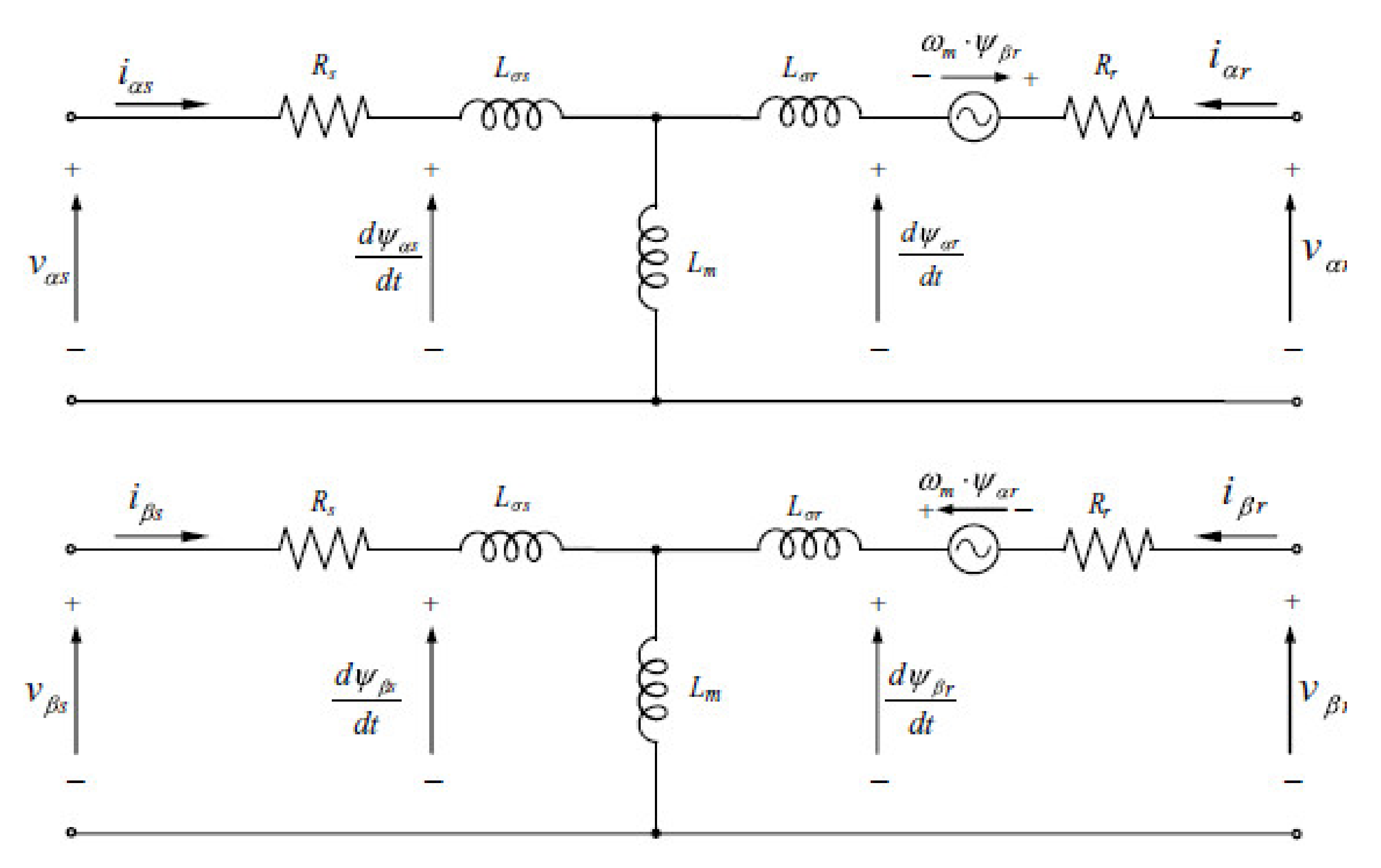
2.1.3. DFIG—Doubly Fed Induction Generator Modeling

The stator ${\overrightarrow{i_{dfig.s}}}^{\mathrm{s}}$ and rotor ${\overrightarrow{i_{dfig.r}}}^{\mathrm{s}}$ current vectors of the WECS DFIG are obtained using the electromagnetic Equations (8)–(10) [15] (pp. 216–217) of an induction machine in the stator reference frame (α, β) operating in generator mode (T_gen ≤ 0) [16] (Figure 2).

$$\dot{{\overrightarrow{i_{\_.s}}}^{\mathrm{s}}}=\frac{\left(-R_{\_.s}·L_{\_.r}-j·{\omega }_{gen}·{\left(L_{\_.m}\right)}^2 \right)·{\overrightarrow{i_{\_.s}}}^{\mathrm{s}}+\left(R_{\_.r}·L_{\_.m}-j·{\omega }_{gen}·L_{\_.m}·L_{\_.r}\right)·{\overrightarrow{i_{\_.r}}}^{\mathrm{s}}+L_{\_.r}·{\overrightarrow{v_{\_.s}}}^{\mathrm{s}}-L_{\_.m}·{\overrightarrow{v_{\_.r}}}^{\mathrm{s}}}{{\sigma }_{\_.}·L_{\_.s}·L_{\_.r}}$$

(8)

$$\dot{{\overrightarrow{i_{\_.r}}}^{\mathrm{s}}}=\frac{\left(R_{\_.s}·L_{\_.m}+j·{\omega }_{gen}·L_{\_.m}·L_{\_.s} \right)·{\overrightarrow{i_{\_.s}}}^{\mathrm{s}}+\left(-R_{\_.r}·L_{\_.s}+j·{\omega }_{gen}·L_{\_.r}·L_{\_.s}\right)·{\overrightarrow{i_{\_.r}}}^{\mathrm{s}}-L_{\_.m}·{\overrightarrow{v_{\_.s}}}^{\mathrm{s}}+L_{\_.s}·{\overrightarrow{v_{\_.r}}}^{\mathrm{s}}}{{\sigma }_{\_.}·L_{\_.s}·L_{\_.r}}$$

(9)

$$\mathrm{with}: {\sigma }_{\_.}=1-\frac{{\left(L_{\_.m}\right)}^2}{L_{\_.s}·L_{\_.r}}$$

(10)

In Equations (8)–(10), “_” stands for DFIG or IM depending on which the Equations refer to. Where ω_gen is the DFIG rotor speed (and the in case that Equations (8)–(10) refer to IM), then ω_gen should be substituted with ω_ps, ${\overrightarrow{v_{\_.s}}}^{\mathrm{s}}$ and ${\overrightarrow{v_{\_.r}}}^{\mathrm{s}}$ are the DFIG/IM stator and rotor voltage vectors, R_.s and R_.r represent the DFIG/IM stator and rotor resistance, and L_._m, L_._s, and L_._r are the DFIG/IM magnetizing, stator, and rotor inductances, respectively.

The electromagnetic torque of the generator T_gen and the generated electrical power P_wecs are calculated using the following Equations (11) and (12) [15] (p. 214):

$$T_{gen}=\frac{3}{2}·p_{gen}·L_m·Im\left\{\overrightarrow{i_{dfig.s}}·{\overrightarrow{i_{dfig.r}}}^{*}\right\}$$

(11)

$$P_{wecs}=P_{gens}+P_{genr}=\frac{3}{2}·Re\left\{\overrightarrow{v_{dfig.s}}·{\overrightarrow{i_{dfig.s}}}^{*}\right\}+\frac{3}{2}·Re\left\{\overrightarrow{v_{dfig.r}}·{\overrightarrow{i_{dfig.r}}}^{*}\right\}$$

(12)

where p_gen represents the generator number of pole pairs, P_gens represents the power delivered by the DFIG stator, and P_genr represents the power delivered by the DFIG rotor.

2.1.4. Tower

The tower dynamics are represented by a mass-spring-damper system where $z$, $\dot{z}$, $\ddot{z}$ represents the deflection, speed, and acceleration of the tower top, respectively [11,12]:

$$m_{wecs}·\ddot{z}=F_{wt}-4·\pi ·m_{wecs}· {\left(f_{ntow}\right)}^2·z-4·\pi · m_{wecs}·f_{ntow}·{\zeta }_{tow}·\dot{z}$$

(13)

In Equation (13), m_wecs represents the WECS mass (including the tower mass), and ${\zeta }_{tow}$ and $f_{ntow}$ represent the tower damping ratio and first eigenfrequency, respectively.

2.1.5. Pitch Actuator

The dynamics of the pitch actuator are modeled using Equation (14) as a second-order system with a time constant τ_β and an input delay λ_β from input u_β to the pitch rate $\dot{\beta }$ [14].

$$\ddot{\beta }=\frac{1}{{\tau }_{\beta }}\left(u_{\beta }^{\lambda }-\dot{\beta }\right)$$

(14)

The pitch actuator is controlled by a proportional regulator with constant K_β (15) [14]:

$$u_{\beta }=K_{\beta }\left({\beta }_{ref}-\beta \right)$$

(15)

where β_ref represents the pitch angle reference.

2.2. Pumping System Modeling

The dynamics of the PS, including the water distribution and irrigation systems, are modeled according to the following equation of motion based on the difference between the pump (load) and motor (electromechanical) torques (T_pump and T_motor) [7,18]:

$$I_{ps}·\dot{{\omega }_{ps}}=T_{motor}-T_{pump}$$

(16)

where I_ps is the moment of inertia of the pumping system, ω_ps is the angular velocity of the shaft connecting the motor and pump, T_motor is the electromechanical torque of the motor, and T_pump is the pump (motor load) torque.

2.2.1. IM (Induction Motor) Modeling

Similar to the DFIG, the electromagnetic torque of the IM T_motor is calculated according to Equation (17) [15] (p. 146), where the IM stator ${\overrightarrow{i_{im.s}}}^{\mathrm{s}}$ and rotor ${\overrightarrow{i_{im.r}}}^{\mathrm{s}}$ current space vectors are obtained based on a model using the same electromagnetic Equations (8)–(10) of an induction machine in the stator reference frame (α, β), but this time operating in motor mode (T_motor ≥ 0)

$$T_{motor}=\frac{3}{2}·p_{motor}·L_{im.m}·Im\left\{\overrightarrow{i_{im.s}}·{\overrightarrow{i_{im.r}}}^{*}\right\}$$

(17)

where p_motor represents the motor number of pole pairs and L_im.m represents the motor magnetizing inductance.

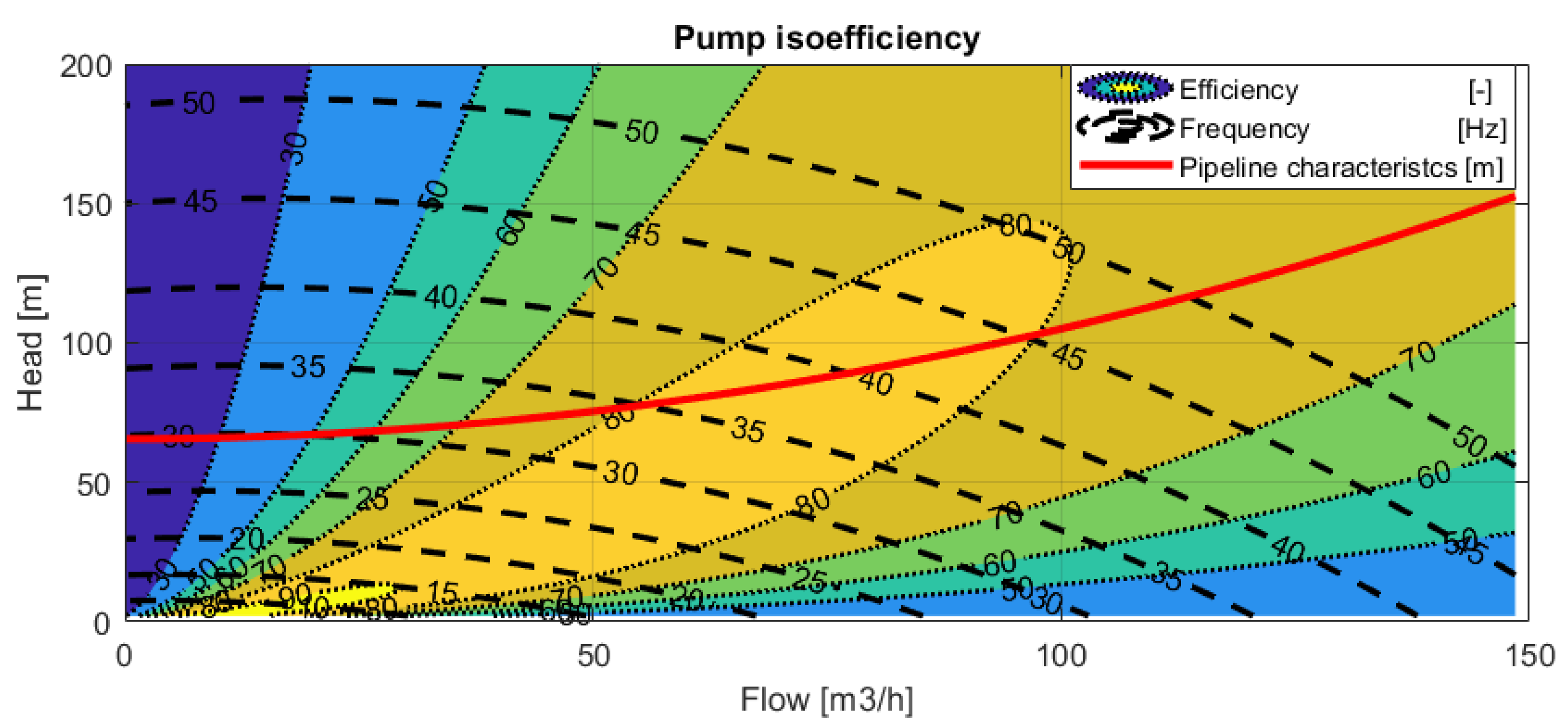
2.2.2. Variable Speed Centrifugal Pump

The pump is modeled based on A, B, and C coefficients identified through quadratic regression (18) from the centrifugal pump characteristic head–flow (H₀-Q₀) curve, and on D and E coefficients also identified through quadratic regression (19) from the efficiency–flow (η₀-Q₀) curve. Both curves (H₀-Q₀ and η₀-Q₀) are at nominal speed (ω_ps0) [4,19,20]. Starting from Equation (18), until Equation (34), including Equations (48)–(52), the subscript “0” stands for the nominal value, and “s” for the current value.

$$H_0=A+B·Q_0+C·{\left(Q_0\right)}^2$$

(18)

$${\eta }_0=D·Q_0+E·{\left(Q_0\right)}^2$$

(19)

where H represents the pump head, Q the pump flow, and η the pump efficiency.

The response of the centrifugal pump to a different speed is modeled using the pump affinity laws (in the current work, the change in water density ${\rho }_{ws}={\rho }_{w0}$ and pump geometry $G_s=G_0$ during the speed variation is ignored) [21] (p. 776):

$$\frac{{\mathrm{Q}}_{\mathrm{s}}}{Q_0}=\frac{{\omega }_{pss}}{{\omega }_{ps0}}·{\left(\frac{G_s}{G_0}\right)}^3; \frac{H_{\mathrm{s}}}{H_0}={\left(\frac{{\omega }_{pss}}{{\omega }_{ps0}}\right)}^2·{\left(\frac{G_s}{G_0}\right)}^2; \frac{P_{\mathrm{pss}}}{P_{ps0}}=\left(\frac{{\rho }_{ws}}{{\rho }_{w0}}\right)·{\left(\frac{{\omega }_{pss}}{{\omega }_{ps0}}\right)}^3·{\left(\frac{G_s}{G_0}\right)}^5;$$

(20)

where P_ps stands for the pumping system power consumption.

By combining the (H₀-Q₀) quadratic regression Equation (17) at nominal speed (ω_ps0) with the pump affinity laws (20), the pump characteristic (H_s-Q_s) as a function of pump speed is obtained (21):

$$H_s={\left(\frac{{\omega }_{pss}}{{\omega }_{ps0}}\right)}^2·A+\left(\frac{{\omega }_{pss}}{{\omega }_{ps0}}\right)·B·Q_s+C·{\left(Q_s\right)}^2$$

(21)

Figure 3 shows the pump characteristic (H_s-Q_s) curve at different speeds (frequency variation from 5 to 50 Hz).

By combining the (η₀-Q₀) quadratic regression of Equation (19) at nominal speed (ω_ps0) with the pump affinity laws (20) using the equation from reference [20], the pump efficiency as a function of pump speed is obtained (22):

$${\eta }_s\left({\omega }_s\right)=1-\left(1-{\eta }_0\right)·{\left(\frac{{\omega }_{ps0}}{{\omega }_{pss}}\right)}^{0.1}=1-{\left(\frac{{\omega }_{ps0}}{{\omega }_{pss}}\right)}^{0.1}+D·Q_s·{\left(\frac{{\omega }_{ps0}}{{\omega }_{pss}}\right)}^{1.1}+E·{\left(Q_s\right)}^2·{\left(\frac{{\omega }_{ps0}}{{\omega }_{pss}}\right)}^{2.1}$$

(22)

2.2.3. Water Distribution and Irrigation System

The water distribution and irrigation system characteristic curve is expressed by equation using [19]:

$$H_s=H_g+k·{\left(Q_s\right)}^2$$

(23)

where H_g is the static head, Q_s is the system flow rate, and k is the head loss coefficient. Figure 3 shows the iso-efficiency diagram of the pump together with the system characteristic curve. The IM pump used for the simulation can be found in reference [22].

The delivered flow as a function of pump speed (ω_ps0) is given by the pump operating point, represented by the cross-point of the pump characteristic as a function of speed (21) with the system characteristic curve (23):

$$H_g+k·{\left(Q_s\right)}^2={\left(\frac{{\omega }_{pss}}{{\omega }_{ps0}}\right)}^2·\mathrm{A}+\left(\frac{{\omega }_{pss}}{{\omega }_{ps0}}\right)·\mathrm{B}·{\mathrm{Q}}_{\mathrm{s}}+C·{\left(Q_s\right)}^2$$

(24)

From which results:

$$Q_s\left({\omega }_{pss}\right)=\frac{-\left(\frac{{\omega }_{pss}}{{\omega }_{ps0}}\right)·\mathrm{B}-\sqrt{{\left(\frac{{\omega }_{pss}}{{\omega }_{ps0}}\right)}^2·{\mathrm{B}}^2-4·\left[{\left(\frac{{\omega }_{pss}}{{\omega }_{ps0}}\right)}^2·\mathrm{A}-{\mathrm{H}}_{\mathrm{g}}\right]·\left(C-k\right)}}{2·\left(C-k\right)}$$

(25)

The pump torque (T_pump) is calculated based on the division of the delivered hydraulic power (P_hydraulic) with the pump speed (ω_pss), taking into consideration the pump efficiency at the operating point (η_s), Equation (26) [23]:

$$T_{pump}=\frac{P_{pump}}{{\omega }_{pss}}=\frac{P_{hydraulic}}{{\omega }_{pss}·{\eta }_s}=\frac{{\rho }_w·g·H_s·Q_s}{{\omega }_{pss}·{\eta }_s}$$

(26)

where ${\rho }_w$ is the water density and $g$ is the gravitational acceleration.

Finally, the pump torque as function pump speed, can be obtained through the substitution of Equations (22), (23), and (25) into Equation (26):

$$T_{pump}=\frac{{\rho }_w·g·H_g·Q_s+\rho ·g·k_1·{\left(Q_s\left({\omega }_{pss}\right)\right)}^3}{{\omega }_{pss}·\left(1-{\left(\frac{{\omega }_{ps0}}{{\omega }_{pss}}\right)}^{0.1}+D·Q_s\left({\omega }_{pss}\right)·{\left(\frac{{\omega }_{ps0}}{{\omega }_{pss}}\right)}^{1.1}+E·{\left(Q_s\left({\omega }_{pss}\right)\right)}^2·{\left(\frac{{\omega }_{ps0}}{{\omega }_{pss}}\right)}^{2.1}\right)}$$

(27)

3. Control Strategy

The control strategy of the PS powered by a WECS was developed according to Figure 1, consisting of three levels of controllers: three first-level controllers, two necessary for the power converters of the WECS generator and one for the pump motor, three second-level controllers, two necessary for the WECS and the one for the PS, and one third-level controller for the general operation of the entire system.

The frequency of the WECS exported power is controlled by the DFIG grid side controller described in Section 3.2.2, and the frequency of the pump’s IM absorbed power is controlled by the IM controller described in Section 3.3.1.

3.1. General System Controller

The general system controller regulates the WECS power demand P_wecsdem according to the pumping pressure reference expressed in pump head H. The controller is developed based on the first-order Tylor polynomial linearization of the affinity laws (20):

$$H_s=H_0+\left({\omega }_{pss}-{\omega }_{ps0}\right)·{(\dot{H})}_{\omega ps0};$$

(28)

By substituting

$$\Delta {\omega }_{ps}=\left({\omega }_{pss}-{\omega }_{ps0}\right) \mathrm{and} \Delta H=\left(H_s-H_0\right)$$

(29)

in Equation (28), results in the following

$$\Delta H=\Delta {\omega }_{ps}·{(\dot{H})}_{\omega ps0}=\Delta {\omega }_{ps}·\frac{2·H_0}{{\omega }_0}; \Delta {\omega }_{ps}=\frac{{\omega }_{ps0}}{2·H_0}·\Delta H$$

(30)

$$P_{pss}=P_{ps0}+\left({\omega }_{pss}-{\omega }_{ps0}\right)·{(\dot{P_{ps}})}_{\omega ps0};$$

(31)

By a similar substitution as in Equation (29), Equation (31) becomes:

$$\Delta P_{ps}=\Delta {\omega }_{ps}·{(\dot{P_{ps}})}_{\omega ps0}=\Delta \omega ·\frac{3·P_{ps0}}{{\omega }_0}$$

(32)

From Equations (30) and (32)

$$\Delta P_{ps}=\frac{3·P_{ps0}}{2·H_0}·\Delta H$$

(33)

The WECS power demand $P_{wecsdem}$ is calculated according to the following:

$$P_{wecsdem}=\left\{\begin{array}{cc}{P}_{ps0}·{\eta }_0& H_s<H_0\\ \left(\frac{3·P_{ps0}}{2·H_0}·\Delta H+P_{ps0}\right)·{\eta }_s& H_s\ge H_0\end{array}\right.$$

(34)

3.2. WECS Controller

The WECS controller was developed based on the combination between the first control level (DFIG including the rotor and grid side controllers) from reference [15,17] with the second control level (WT controller) from reference [14], with several modifications to adapt the WECS power production to the pumping system operating point.

The first control level consists of two modulator controllers that regulate the convertors switch pulses to the desired reference values, to ensure proper and effective power generation.

3.2.1. DFIG Rotor Side Controller

The DFIG rotor side controller consists of a rotor flux-oriented vector controller that controls the modulator generating the rotor converter switch pulses necessary for maintaining the magnitudes of the generator (such as torque, active, and reactive power) close to their optimum values.

The DFIG rotor flux-oriented vector control regulates the d-q rotor currents by using a regulator for each current component and is mainly performed according to reference [17] (p. 283) with several modifications.

The gains for the proportional-integral (PI) regulators for the current loops are calculated in Equations (35) and (36) according to the second-order system with two poles and one zero presented in reference [17] (p. 282).

$$k_{pr}=\frac{2·100·\left({\sigma }_{DFIG}\right){ }^2 ·{\left(L_{DFIG.r}\right)}^2}{R_{DFIG.r}}-R_{DFIG.r}$$

(35)

$$k_{ir}=\frac{10000·\left({\sigma }_{DFIG}\right){ }^3·{\left(L_{DFIG.r}\right)}^3}{{\left(R_{DFIG.r}\right)}^2}$$

(36)

where k_pr is the proportional gain of the DFIG rotor side regulator, k_ir is the integral gain of the DFIG rotor side regulator, L_DFIG.r is the rotor inductance, R_DFIG.r is the rotor resistance, and σ_DFIG can be found in Equation (10).

3.2.2. DFIG Grid Side Controller

The DFIG grid side controller consists of a grid voltage-oriented vector controller that regulates the modulator generating the rotor converter switch pulses necessary for maintaining the magnitudes of the grid side converter (such as the reactive power and the DC bus voltage) close to their optimum values.

The DFIG grid voltage-oriented control regulates the voltage (Vbus) of the DC link (mainly formed by a capacitor) so that part of the WECS generated power can be delivered through the rotor. Therefore, by only maintaining the Vbus variable at a constant value, this active power flow through the converters is ensured, together with a guarantee that both grid and rotor side converters have the required DC voltage needed to work properly [15]. The DFIG grid voltage-oriented control is implemented according to reference [15] (p. 146), [20] (p. 178).

The gains for the proportional-integral (PI) regulators for the current loops are calculated in Equations (38) and (39) according to the closed-loop current expressions, from reference [24] (p. 180).

$$s^2·\left(L_f\right)+s·\left(R_f+k_{pg}\right)+k_{ig}\equiv s^2+2·{\xi }_1·{\omega }_{n1}·s+{\left({\omega }_{n1}\right)}^2$$

(37)

From which results:

$$k_{pg}=2·L_f·{\xi }_1·{\omega }_{n1}-R_f$$

(38)

$$k_{ig}=L_f·{\left({\omega }_{n1}\right)}^2$$

(39)

where k_pg is the proportional gain or the DFIG grid side regulator, k_ig is the integral gain of the DFIG gride side regulator, and L_f is the grid side filter inductance; R_f is the grid side filter resistance, and ωn1 and ${\xi }_1$ are the first natural frequency and damping ratio of the closed-loop system, respectively, Equation (37).

The second control level, called the WT controller, consists of two controllers—the generator torque controller and the blade pitch controller.

3.2.3. WT Generator Torque Controller

A WT generator-torque (partial load) controller, that maximizes the power capture below the rated operation point, while the blade pitch is kept constant at 0 (β_ref = 0°) (the WT generator-torque controller was developed by combining [1,13,15,25]) can be represented as:

$$\begin{gathered} T_{gen.ctr}\left({\omega }_{gen}\right)=\left\{\begin{array}{cc}0,& {\omega }_{gens}\le {\omega }_{cut.in}\hspace{1em}or v_{rot}>v_{cutout}\\ a_{1–2}·{\omega }_{gen}+b_{1–2} ,& {\omega }_{cut.in}<{\omega }_{gens}<{\omega }_{optimal}\\ k_{opt}·{\left({\omega }_{gen}\right)}^2,& {\omega }_{opt}\le {\omega }_{gens}\le {\omega }_{ms}\\ a_{2–3}·{\omega }_{gen}+b_{2–3},& {\omega }_{ms}<{\omega }_{gens}<{\omega }_{gen0}\end{array}\right. \\ {\beta }_{ref}=0° \end{gathered}$$

(40)

Equation (40) is taken into consideration when $P_{wecsdem}\ge P_{wecs0} AND {\omega }_{gens}<{\omega }_{gen0}$, where v_rot is the average wind speed over the rotor; v_cutout is the cutout wind speed over the rotor; T_gen.ctr is the controller desired generator torque; ω_gen is the generator speed; P_wecsdem the WECS demanded power; P_wecs0 the WECS actual power; η_gen the rated generator efficiency; ω_cut.in the generator angular velocity at cut-in wind speed; ω_optimal the generator angular velocity at optimal tip speed ratio; ω_ms the generator rotor mechanical speed at synchronous stator speed.; ω_gens the actual generator angular velocity; ω_gen0 the rated generator angular velocity; and β_ref the reference pitch angle.

a_1–2 and b_1–2 represent the coefficients of the linear equation between regions 1 and 2 in Figure 4:

$$a_{1–2}=\frac{k_{opt}·{\left(1.3·{\omega }_{cut.in}\right)}^2}{0.3·{\omega }_{cut.in}}$$

(41)

$$b_{1–2}=-a_{1–2}·{\omega }_{cut.in}$$

(42)

$$\mathrm{With} k_{opt}=\frac{1}{2}·\frac{R^5}{{\left({\lambda }_{peak}\right)}^3·N^3}·\rho ·\pi ·C{p}_{peak}$$

(43)

where Cp_peak is the power coefficient peak value when pitch angle = 0° and k_opt is the optimal constant that also corresponds to the optimal generator torque in Figure 4:

$$\mathrm{With} T_{genoptimal}=k_{opt}·{\left({\omega }_{gens}\right)}^2$$

(44)

Similar to Equations (41) and (42), in Equations (45)–(46) a_2–3 and b_2–3 represent the coefficients of the linear equation between regions 2 and 3 in Figure 4:

$$a_{2–3}=\frac{T_{gen0}-k_{opt}·{\left({\omega }_{ms}\right)}^2}{99\%·{\omega }_{gen0}-{\omega }_{ms}}$$

(45)

$$b_{2–3}=k_{opt}·{\left({\omega }_{ms}\right)}^2-a_{2–3}·{\omega }_{ms}$$

(46)

Figure 4 shows the controller generator torque reference, T_gen.ctrl in Equation (40), as a function of the filtered generator speed.

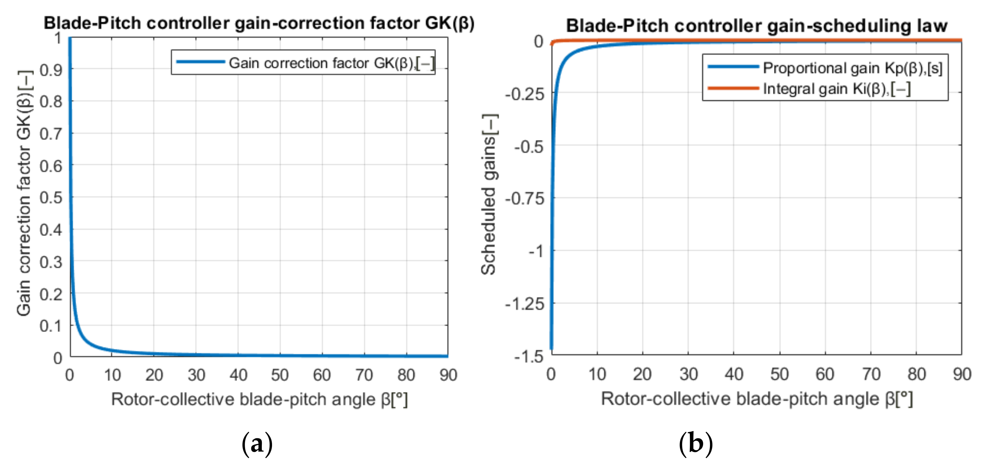
3.2.4. WT Blade Pitch Controller

The second WT controller is a rotor-collective blade-pitch (full load) controller that starts its operation when the aerodynamic power is higher than the demanded power and has the goal to indirectly regulate the generator speed to the rated speed, and directly regulate the rotor speed by pitching the blades. Because the sensitivity (the first derivative) of the aerodynamic torque to the rotor-collective blade pitch varies nearly linearly with the blade-pitch angle [17], constant PI gains are not adequate for effective speed control and a linear gain correction with the same slope as the rotor torque sensitivity (a function of the blade-pitch angle) is implemented.

$$K{p}_{wecs}\left(\begin{array}{c}\beta \end{array}\right)=K{p}_{wecs}·GK\left(\begin{array}{c}\beta \end{array}\right)$$

(47)

$$K{i}_{wecs}\left(\begin{array}{c}\beta \end{array}\right)=K{i}_{wecs}·GK\left(\begin{array}{c}\beta \end{array}\right)$$

(48)

where:

Kp_wecs(β) and Ki_wecs(β) are the controller’s proportional and integral gains, respectively, at β pitch angle, and

Kp_wecs and Ki_wecs are the base pitch controller proportional and integral gains, respectively, at the rated operation point.

$GK\left(\begin{array}{c}\beta \end{array}\right)=\frac{1}{1+\frac{\beta }{{\beta }_k}}$ is the linear gain correction factor, based on the blade-pitch angle according to reference [25], in which β [in radians in this formula] is the pitch angle and βk [radians/s] is the pitch angle where the pitch sensitivity has doubled.

The pitch angle where the rotor torque sensitivity as a function of blade-pitching angle has doubled (β_k) is calculated from Equation (3), after being linearized with the Taylor expansion series:

$$2·T_{wt0}=T_{wt0}+{\left.\frac{\partial T_{wt}}{\partial \beta }\right|}_{\left(v_{rot0},{\omega }_{wt0},{\beta }_0\right)}·\left({\beta }_0-{\beta }_k\right)$$

(49)

$${\beta }_k={\beta }_0-\frac{T_{wt0}}{{\left.\frac{\partial T_{wt0}}{\partial \beta }\right|}_{\left(v_{rot0},{\omega }_{wt0},{\beta }_0\right)}}$$

(50)

where: T_wt is the rotor torque at linearization point ($T_{wt0}$ being the rated value); β₀ = 0 is the rated pitch angle in the rated operation point, βk [rad/s] is the pitch angle where the rotor torque sensitivity has doubled, $v_{rot0}$ is the average wind speed over the rotor, and ${\omega }_{wt0}$ is the angular rotor velocity.

Figure 5 shows the wind turbine blade-pitch controller gain correction factor [GK(β)] and the gain scheduling law.

By combining a blade-pitching angle PI closed-loop equation with the linear gain correction Equation (49), the final closed-loop equation is obtained:

$$\begin{array}{c}{T}_{gen.ctr}\left({\omega }_{gens}\right)=\frac{P_{wecs0}}{{\omega }_{gens}·{\eta }_{gen}}, \\ {\begin{array}{c}\beta \end{array}}_{ref}=\frac{{\beta }_k}{{\beta }_k+{\beta }_{ref}}·K{p}_{wecs}·{\omega }_{err}+\frac{{\beta }_k}{{\beta }_k+{\beta }_{ref}}·K{i}_{wecs}·\int {\omega }_{err},\end{array}$$

(51)

Equation (51) is taken into consideration when $P_{wecsdem}\le P_{wecs0} OR {\omega }_{gens}\ge {\omega }_{gen0}$ where β_ref is the reference pitch angle; βk is the pitch angle where the pitch sensitivity has doubled; Kp_wecs and Ki_wecs are the pitch controller proportional and integral gains, respectively, at the rated operation point; and ω_err = ω_rated-ω represents the difference between the rated and actual generator angular velocity.

In the blade-pitch controller, there is a conditional statement for setting as a reference for the upper limit of the blade-pitch angle when the wind speed in front of the rotor reaches the cutout wind speed.

3.3. Pumping System Controller

The PS controller was developed based on the combination of the first control level (IM controller) from reference [24] and the second control level (pump speed controller) from reference [26].

Because the pump system controller is in cascade with the WECS controller, the produced power by the WECS is passed to the PS controller, based on which the PI controlled error ${\omega }_{pserr}$ (the difference between the reference and current pump speed) is calculated using Equation (29):

$${\omega }_{PSerr}=\left\{\begin{array}{cc}-{\omega }_{pss}& P_{wecs}<P_{psmin}\\ \frac{{\omega }_{ps0}}{3·P_{ps0}}·\left(P_{wecs}-P_{pss}\right)& P_{wecs}\ge P_{psmin}\end{array}\right.$$

(52)

where P_psmin represents the minimum power required by the pump motor to work properly; in this particular case, for pumping the minimum flow required by the pump motor for cooling.

3.3.1. IM Controller

The IM motor controller uses a standard solution for current regulation in vector-controlled AC drives [24] (p. 59), called the synchronous PI current regulator, with two independent regulators, one for the d and one for the q axis.

The synchronous PI current regulators are tuned using a second-order equivalent system presented in reference [24] (p. 61):

$$s^2·\left({\sigma }_{IM}·L_{IM.s}\right)+s·\left(R_{IM.s}+k_{pps}\right)+k_{ips}\equiv s^2+2·{\xi }_2·{\omega }_{n2}·s+{\left({\omega }_{n2}\right)}^2$$

(53)

$$k_{pps1}={\sigma }_{IM}·L_{IM.s}·2·{\xi }_2·{\omega }_{n2}-R_{IM.s}$$

(54)

$$k_{ips1}={\sigma }_{IM}·L_{IM.s}·{\left({\omega }_{n2}\right)}^2$$

(55)

$$\mathrm{with} {\sigma }_{IM}=1-\frac{{\left(L_{IM.m}\right)}^2}{L_{IM.s}·L_{IM.r}}, {\xi }_2=1, {\omega }_{n2}=\frac{10}{\frac{{\sigma }_{IM}·L_{IM.s}}{R_{IM.s}}}$$

(56)

where $k_{pps1}$ represents the proportional gain of the IM motor PI controller; $k_{ipps1}$ represents the integral gain of the IM motor PI controller; ω_n2 and ${\xi }_2$ are the first natural frequency and damping ratio, respectively, of the closed-loop system, Equation (53), and the most suitable double real poles of the closed-loop system (-ω_n2) were identified by trial and error to be $\frac{10}{\frac{{\sigma }_{IM}·L_{IM.s}}{R_{IM.s}}}$.

3.3.2. Pump Speed Controller

The speed control loop provides the frequency reference to the induction motor controller. The speed regulator is a PI type and is tuned taking into account the following second-order equivalent system:

$$s^2·\left(\frac{2·\pi }{p_{motor}}·I_{ps}\right)+s·k_{pps2}+k_{ips2}=s^2+2·{\xi }_3·{\omega }_{n3}·s+{\left({\omega }_{n3}\right)}^2$$

(57)

with

$$k_{pps2}=\frac{2·\pi }{p_{motor}}·I_{ps}·2·{\xi }_3·{\omega }_{n3}$$

(58)

$$k_{ips2}=\frac{2·\pi }{p_{motor}}·I_{ps}·{\left({\omega }_{n3}\right)}^2$$

(59)

where $k_{pps2}$ represents the proportional gain of the PS speed controller; $k_{ips2}$ represents the integral gain of the PS speed controller; ω_n3 and ${\xi }_3$ are the first natural frequency and damping ratio, respectively, of the closed-loop system in Equation (57).

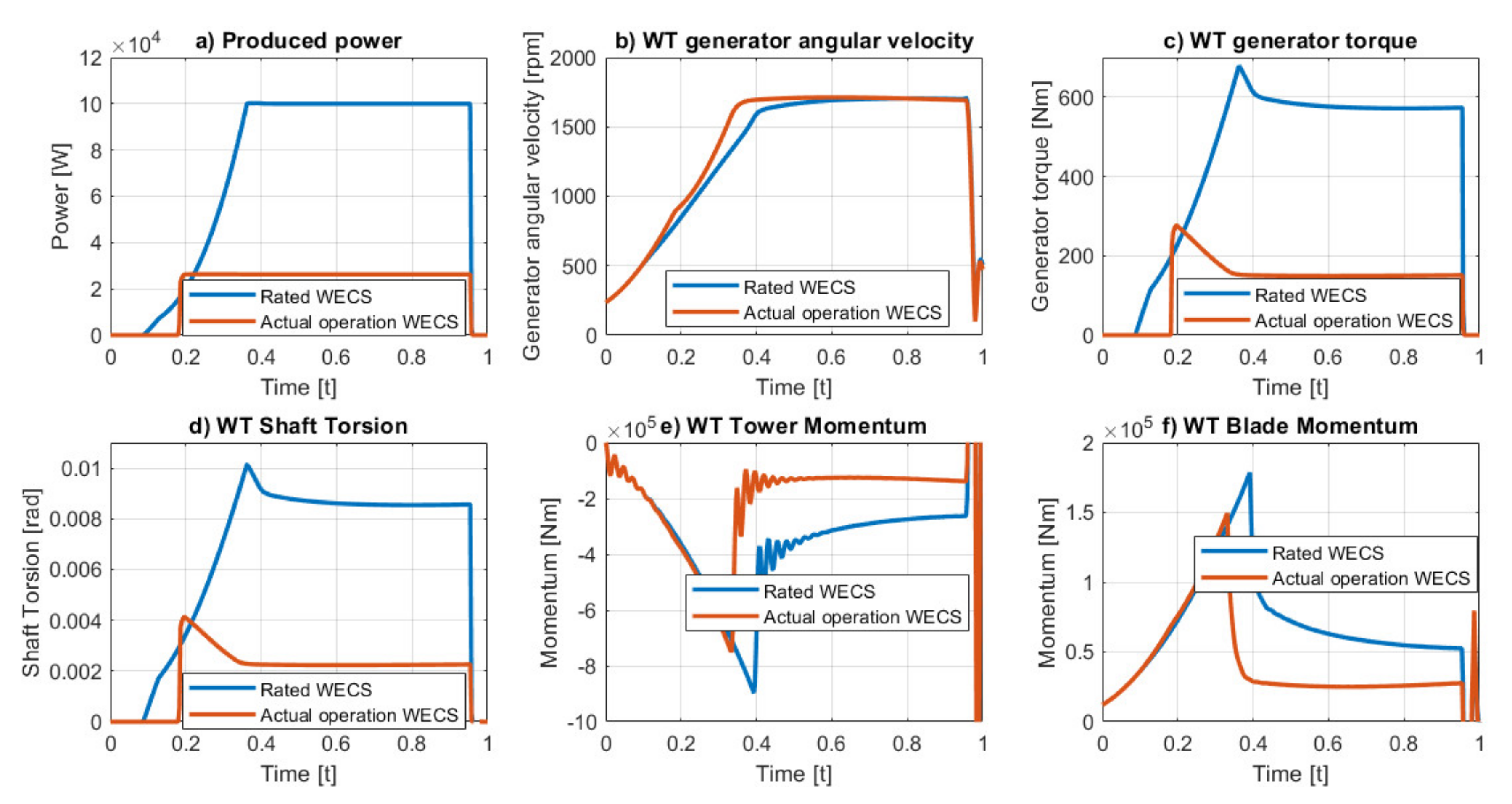
4. Simulation Results and Discussions

Several simulations depicting different circumstances were conducted to determine how the presented control responds. The input parameters necessary for modeling, defining the controller, and running the simulation are presented in

Table A1. Necessary parameters for modeling, defining. the controller and running the simulations [22,27].

Component	Notation	Parameter Description	Value
WECS WT	v	Wind speed in front of the WT rotor	4 to 26 [m/s]
	vrot	Average wind speed acting on the WT rotor	4 to 26 [m/s]
	vcut.in	Cut-in wind speed in front of the WT rotor	5 [m/s]
	vrated	Rated wind speed in front of the WT rotor	13 [m/s]
	vcut.out	Cut out wind speed in front of the WT rotor	25 [m/s]
	v	Wind speed in front of the WT rotor	4 to 26 [m/s]
	$\lambda$	WT rotor tip speed ratio	3.923 [rad/s]
	R	WT rotor radius	10.5 [m]
	${\omega }_{wt}$	Nominal WT rotor angular velocity	4.857 [rad/s]
	$T_{wt}$	Nominal WT rotor torque	20,588 [N·m]
	${\rho }_{air}$	Average air density over the WT rotor	1.2231 [kg/m3]
	$C_p$	Power coefficient lookup table [27]	[-]
	$C_T$	Thrust coefficient lookup table [27]	[-]
	$\beta$	Nominal blade pitching angle	0 [°]
	$H_{hub}$	WT hub height	38 [m]
WECS Drive Train	$I_{wt}$	WT rotor inertia	115,762 [kg·m2]
	$K_{shaft}$	WT low-speed shaft spring constant	2,208,535 [N·m/rad]
	$B_{sfhat}$	WT low-speed shaft damping constant	15,820 [kg/s]
	N	Gear ratio	33 [-]
WECS DFIG	$I_{gen}$	DFIG inertia	10.682 [kg·m2]
	$p_{gen}$	DFIG poles	4 [-]
	udfig	DFIG stator/rotor turns ratio	1 [-]
	fdfig	DFIG rated frequency	50 [Hz]
	Vdfig	DFIG rated voltage	400 [V]
	Idfig	DFIG rated current	145 [A]
	${\omega }_{gen}$	DFIG rated angular velocity	1500 [rpm]
	Rdfig.S	DFIG stator resistance	0.08 [Ω]
	Rdfig.R	DFIG rotor resistance	0.008 [Ω]
	Ldfig.m	DFIG magnetizing induction	0.007 [H]
	Ldfig.R	DFIG rotor inductance	0.074 [H]
	Ldfig.S	DFIG stator inductance	0.074 [H]
	Vbus	DC bus voltage referred to the DFIG stator	690 [V]
	Pwecs	DFIG rated power	100 [kW]
WECS Tower	mwecs	WECS mass	21 [tons]
	$H_{tow}$	Tower height	35 [m]
	${\zeta }_{tow}$	Tower damping ratio	0.08 [-]
	$f_{ntow}$	Tower first eigenfrequency	0.35 [Hz]
WECS Pitch Actuator	τβ	Pitch actuator time constant	0.1 [s]
	λβ	Pitch actuator delay	0.1 [s]
	Kβ	Proportional gain of the Pitch regulator	10 [-]
	βref	Pitch angle reference	0 [°]
PS IM	$P_{IM}$	IM rated power	51 [kW]
	$p_{IM}$	IM poles	2 [-]
	uIM	IM stator/rotor turns ratio	1 [-]
	fdfig	IM rated frequency	50 [Hz]
	Vdfig	IM rated voltage	400 [V]
	Idfig	IM rated current	101 [A]
	${\omega }_{IM}$	IM rated angular velocity	2910 [rpm]
	Rim.s	IM stator resistance	0.095 [Ω]
	Rim.r	IM rotor resistance	0.063 [Ω]
	Lim.m	IM magnetizing induction	0.032 [H]
	Lim.r	IM rotor inductance	0.034 [H]
	Lim.s	IM stator inductance	0.034 [H]
PS Centrifugal Pump	Pdem	Nominal power demanded by PS to WECS	32.357 [kW]
	Pps	Nominal PS power	26.2 [kW]
	${\omega }_{PS}$	Pump nominal angular velocity	2400 [rpm]
	A	Pump characteristic curve 1st coefficient	185.212 [m]
	B	Pump characteristic curve 2nd coefficient	0.261 [h/m2]
	C	Pump characteristic curve 3rd coefficient	−0.008 [h2/m5]
	D	Pump efficiency curve 1st coefficient	1.8274 [h/m3]
	E	Pump efficiency curve 2nd coefficient	−0.0104 [h2/m6]
	H0	Nominal pump operating head	87.312 [m]
	Q0	Nominal pump operating flow	86.56 [m3/h]
	η0	Nominal pump efficiency	0.81 [-]
	k	Head loss coefficient	0.00395 [h2/m5]
	Hg	Static head	80.5 [m]

of Appendix A. All the gains and parameters of the controller are presented in

Table A2. Calculated controller parameters.

Local Controller	Notation	Parameter Description	Value
WECS DFIG rotor side controller	kpr	P gain of the DFIG rotor side regulator	0.0635 [-]
	kir	I gain of the DFIG rotor side regulator	0.635 [-]
WECS DFIG grid side controller	kpg	P gain of the DFIG grid side regulator	0.002 [-]
	kig	I gain of the DFIG grid side regulator	−0.002 [-]
WECS WT generator torque controller	$k_{opt}$	Optimal generator constant	0.0314 [-]
	$a_{1–2}$	1st linear coefficient Equations (1) and (2) region	8.34 [-]
	$b_{1–2}$	2nd linear coefficient Equations (1) and (2) region	−393.174 [-]
	$a_{2–3}$	1st linear coefficient Equations (2) and (3) region	34.823 [-]
	$b_{2–3}$	2nd linear coefficient Equations (2) and (3) region	−4889.242 [-]
WECS WT blade pitch controller	Kpwecs	Pitch controller P gain at the rated point	−0.7395 [-]
	Kiwec	Pitch controller I gain at the rated point	−0.0129 [-]
PS IM controller	kpps1	P gain of the PS IM controller	120 [-]
	kips1	I gain of the PS IM controller	12,000 [-]
PS Pump speed controller	kpps2	P gain of the PS pump speed controller	1 [-]
	kips2	I gain of the PS pump speed controller	1.2 [-]

of Appendix A. The scenario depicted in the current paper illustrates how the PS responds with an available power produced by a WECS during a wind speed ramp from 4 to 26 m/s (the considered WECS operates under normal conditions and when the demanded power equals the rated power, in a wind speed ranging from 5 to 25 m/s). Figure 6 shows the blade-pitching angle operation of the WECS (when the demanded power equals the actual power, necessary for operating the pumping system at its rated power).

Figure 7 shows the response of the key parameters in the operation of the PS powered by the WECS.

Figure 7a shows the WECS theoretical produced power (blue), the pump, and motor power (red and yellow). This diagram illustrates the maximum power point tracking operating at partial load when the power consumption of the PS motor follows the WECS produced power received as a reference in cascade (time from 20 to 40 s), and the pressure regulator (the PI controller that regulates the WECS power demand according to the pumping pressure reference) is operating at full-load (time from 40 to 115 s);

Figure 7b shows the efficiencies of each subsystem integrated into the PS powered by the WECS (blue—wind turbine, red—WECS generator, yellow—pump motor efficiency, purple—pump efficiency, green—the entire system efficiency);

Figure 7c shows the flow pumped by the system, and Figure 7d shows the head of the pump and the pressure reference expressed in the pump head.

Figure 8 presents a comparison between the response of the same WECS (more details can be found in reference [27]), operating when the demanded power is equal to the rated power (as a WECS operating in a wind farm with the purpose of injecting all the energy into the grid), and operating when the demanded power is the power required by the pump for its rated operation (the rated power of the pump has to be lower than the rated power of the WECS).

Figure 8a presents the power produced by the WECS when the demanded power is equal to the rated power of the WECS (blue), and the rated power of the PS (red). Figure 8b shows the WECS generator angular velocity in both operating conditions presented above. It can be observed that, when the demanded power from the WECS is lower than the rated power, the WECS generator angular velocity reaches its nominal point faster.

In Figure 8c, it can be observed that the WECS power is derated mainly by derating the WT and generator torque in order to reduce the loads taken by the drive train (WT and WECS generator torques are adapted to the motor power). This fact is also confirmed by Figure 8d, where it can be seen that the torsion of the drive shaft is reduced proportionally to the derating power.

Figure 8e,f shows that how the proposed control strategy for the PS powered by a WECS also considers the loads of the WECS, as the tower and blades moments are reduced proportionally with the WECS power derated to the necessary power required by the PS for its rated operation.

5. Conclusions

This paper shows the application of leading-edge technology within the area of an irrigation PS powered by a pitching WECS, by presenting an advanced dynamic model of the entire system in the first, a system control strategy, and, finally, the simulation results.

The advanced dynamic model developed in this paper includes the main components of a WECS (a WT including pitchable blades and their actuator, its drive train and tower, and a DFIG together with its power converter) and of an irrigation PS (a centrifugal pump, an IM with its power converter, and an irrigation network with a pressure transducer).

The implemented system control strategy is based on local controllers distributed on three levels: a general controller that regulates the WECS power demand according to the pumping pressure reference; three second-level controllers; two necessary for controlling the WT generator torque and speed, and one for controlling the pump speed; and three first-level controllers—two for controlling the DFIG power converters of the WECS and one for controlling the IM power converter of the pump.

Finally, the results depicting the simulations of a general operation of the system covering its transition through the entire operation range showed the good performance and effectiveness of the developed control system strategy. The simulation results presented in Figure 7 and Figure 8 confirm the contribution of the current work in controlling a PS powered by a WECS, the regulation of the pump speed so that the PS consumption power tracks the WECS produced power (Equation (52)) at partial load, and the regulation of the WECS power demand to control the head pressure of the PS (Equation (34)) at full load. The simulation results illustrated in Figure 8 show that, at full load operation, the WECS produces only the power necessary for the rated operation of the PS, in order to avoid unnecessary loading of the WECS components.

The main contribution of the current work compared to other related work [7,8,9,10] consists of integrating a commercial WECS, without altering its hardware or controller, into an existing pumping system. The main reason why most WECS manufacturers are not open to adjusting their current control strategies for a full and perfect integration within a PS is because such an adjustment represents a significant cost, and the WECS manufacturers do not believe the current market for a PS that requires a WECS is large enough to pay this cost. Nevertheless, the unintrusive proposed control strategy system and the promising simulations results indicate the possibility for the application of the proposed scheme to be set up for online implementation.

References

1. Stoyanov, L.; Bachev, I.; Zarkov, Z.; Lazarov, V.; Notton, G. Multivariate Analysis of a Wind–PV-Based Water Pumping Hybrid System for Irrigation Purposes. Energies 2021, 14, 3231. [Google Scholar] [CrossRef]
2. Ursachi, A.; Bordeasu, D. Smart Grid Simulator, World Academy of Science, Engineering and Technology. Int. J. Civ. Archit. Sci. Eng. 2014, 8, 488–491. [Google Scholar] [CrossRef]
3. Ronad, B.F.; Jangamshetti, S.H. Optimal cost analysis of wind-solar hybrid system powered AC and DC irrigation pumps using HOMER. In Proceedings of the 2015 International Conference on Renewable Energy Research and Applications (ICRERA), Palermo, Italy, 22–25 November 2015; Volume 5, pp. 1038–1042. [Google Scholar] [CrossRef]
4. Sarasúa, J.I.; Martínez-Lucas, G.; Platero, C.A.; Sánchez-Fernández, J.Á. Dual Frequency Regulation in Pumping Mode in a Wind–Hydro Isolated System. Energies 2018, 11, 2865. [Google Scholar] [CrossRef] [Green Version]
5. Jamii, J.; Mimouni, F. Model of wind turbine-pumped storage hydro plant. In Proceedings of the 2018 9th International Renewable Energy Congress (IREC), Hammamet, Tunisia, 20–22 March 2018; pp. 1–6. [Google Scholar] [CrossRef]
6. Li, H.; Zheng, C.; Lv, S.; Liu, S.; Huo, C. Research on optimal capacity of wind power based on coordination with pumped storage power. In Proceedings of the 2016 IEEE PES Asia-Pacific Power and Energy Engineering Conference (APPEEC), Xi’an, China, 25–28 October 2016; pp. 1214–1218. [Google Scholar] [CrossRef]
7. Ouchbel, T.; Zouggar, S.; Elhafyani, M.L.; Seddik, M.; Oukili, M.; Aziz, A.; Kadda, F.Z. Power maximization of an asynchronous wind turbine with a variable speed feeding a centrifugal pump. Energy Convers. Manag. 2014, 78, 976–984. [Google Scholar] [CrossRef]
8. Barara, M.; Bennassar, A.; Abbou, A.; Akherraz, M.; Bossoufi, B. Advanced Control of Wind Electric Pumping System for Isolated Areas Application. Int. J. Power Electron. Drive Syst. 2014, 4, 567–577. [Google Scholar] [CrossRef]
9. Zeddini, M.A.; Pusca, R.; Sakly, A.; Mimouni, M.F. MPPT control of Wind Pumping Plant Using Induction Generator. In Proceedings of the 14th International conference on Sciences and Techniques of Automatic Control & Computer Engineering STA, Sousse, Tunisia, 20–22 December 2013; pp. 438–442. [Google Scholar]
10. Harrouz, A.; Dahbi, A.; Harrouz, O.; Benatiallah, A. Control of wind turbine based of PMSG connected to water pumping system in South of Algeria. In Proceedings of the 3rd International Symposium on Environmental Friendly Energies and Applications (EFEA), Paris, France, 19–21 November 2014; pp. 22–25. [Google Scholar] [CrossRef]
11. Hammerum, H. A Fatigue Approach to Wind Turbine Control; Technical University of Denmark: Kongens Lyngby, Denmark, 2006; pp. 5–22. [Google Scholar]
12. Hammerum, H.; Brath, P.; Poulsen, N.K. A fatigue approach to wind turbine control. J. Phys. Conf. Ser. 2007, 75, 012081. [Google Scholar] [CrossRef] [Green Version]
13. Zhang, C.; Wang, L.; Li, H. Experiments and Simulation on a Late-Model Wind-Motor Hybrid Pumping Unit. Energies 2020, 13, 994. [Google Scholar] [CrossRef] [Green Version]
14. Grunnet, J.D.; Soltani, M.N.; Knudsen, T.; Kragelund, M.N.; Bak, T. Aeolus Toolbox for Dynamics Wind Farm Model, Simulation and Control. In Proceedings of the European Wind Energy Conference and Exhibition, EWEC 2010: Conference Proceedings, Warszawa, Poland, 20–23 April 2010; pp. 3119–3129. [Google Scholar]
15. Abad, G.; López, J.; Rodríguez, M.A.; Marroyo, L.; Iwanski, G. Doubly Fed Induction Machine: Modeling and Control for Wind Energy Generation; John Wiley & Sons: Hoboken, NJ, USA, 2011; pp. 155–238. [Google Scholar]
16. Haţiegan, C.; Chioncel1, C.P.; Răduca, E.; Popescu, C.; Pădureanu, I.; Jurcu, M.R.; Bordeaşu, D.; Trocaru, S.; Dilertea, F.; Bădescu, O.; et al. Determining the operating performance through electrical measurements of a hydro generator. IOP Conf. Ser. Mater. Sci. Eng. 2017, 163, 012031. [Google Scholar] [CrossRef] [Green Version]
17. Abu-Rub, H.; Malinowski, M.; Al-Haddad, K. Power Electronics for Renewable Energy Systems, Transportation and Industrial Applications; IEEE Press and John Wiley & Sons Ltd.: Chichester, UK, 2014; pp. 277–356. [Google Scholar]
18. Janevska, G.; Bitola, R.M. Mathematical Modeling of Pump System. Electron. Int. Interdiscip. Conf. 2013, 2, 455–458. [Google Scholar]
19. Yang, Z.; Soleiman, K.; Løhndorf, B. Energy Efficient Pump Control for an Offshore Oil Processing System. IFAC Proc. Vol. 2012, 45, 257–262. [Google Scholar] [CrossRef] [Green Version]
20. Sârbu, I.; Borza, I. Energetic optimization of water pumping in distribution systems. Period. Polytech. Ser. Mech. Eng. 1998, 42, 141–152. [Google Scholar]
21. White, F.M. Chapter 11 Turbomachinery. In Fluid Mechanics, 7th ed.; McGraw-Hill: New York, NY, USA, 2011; pp. 776–777. [Google Scholar]
22. Caprari, Submersible Electric Pump E8P95/7ZC+MAC870-8V Technical Data Sheet. 2019. Available online: https://ipump.caprarinet.net/ (accessed on 9 October 2021).
23. Li, W.; Ji, L.; Shi, W.; Zhou, L.; Chang, H.; Agarwal, R.K. Expansion of High Efficiency Region of Wind Energy Centrifugal Pump Based on Factorial Experiment Design and Computational Fluid Dynamics. Energies 2020, 13, 483. [Google Scholar] [CrossRef] [Green Version]
24. Abad, G. Power Electronics and Electric Drives for Traction Applications; John Wiley & Sons: Chichester, UK, 2017; pp. 37–98, 149–185. [Google Scholar]
25. Jonkman, J.; Butterfield, S.; Musial, W.; Scott, G. Definition of a 5-MW Reference Wind Turbine for Offshore System Development; National Renewable Energy Laboratory: Golden, CO, USA, 2009; pp. 17–27.
26. Sul, S. Control of Electric Machine Drive Systems; John Wiley & Sons: Hoboken, NJ, USA, 2011; pp. 92–96, 236–243. [Google Scholar]
27. Fuhrländer, F.L. Fuhrländer FL 100 kW Wind Turbine Technical Data Sheet. 2021. Available online: https://en.wind-turbine-models.com/turbines/279-fuhrlaender-fl-100-astos/ (accessed on 9 October 2021).
Figure 1. Proposed PS powered by the WECS control structure.
Energies 14 07696 g001
Figure 2. DFIG model (equivalent circuit) in the α-β reference frame [17] (p. 278).
Energies 14 07696 g002
Figure 3. Pump iso-efficiency curve (Hs-Qs-ηs).
Energies 14 07696 g003
Figure 4. Generator-torque controller diagram.
Energies 14 07696 g004
Figure 5. WT blade-pitch controller (a) gain correction factor GK(β); (b) gain scheduling law.
Energies 14 07696 g005
Figure 6. Pitch angle variation during the wind speed ramp.
Energies 14 07696 g006
Figure 7. Simulation results: (a) WECS power production and PS power consumption; (b) efficiency of each subsystem in the PS powered by the WECS; (c) pump flow; (d) pump head including its reference.
Energies 14 07696 g007
Figure 8. Rated vs actual operation of the WECS comparison: (a) power production comparison; (b) generator angular velocity comparison; (c) generator torque comparison; (d) drive train torsion comparison; (e) tower momentum comparison; (f) blade momentum comparison.
Energies 14 07696 g008
Publisher’s Note: MDPI stays neutral with regard to jurisdictional claims in published maps and institutional affiliations.