Research on a Bi-Level Collaborative Optimization Method for Planning and Operation of Multi-Energy Complementary Systems

Abstract

Multi-energy complementary systems (MCSs) are complex multilevel systems. In the process of system planning, many aspects—such as power planning, investment cost, and environmental impact—should be considered. However, different decision makers tend to have different levels of control objectives, and the multilevel problems of the system need to be solved effectively with comprehensive judgment. Therefore, based on the terminal MCS energy structure model, the optimization method of MCS planning and operation coordination, considering the influence of planning and operation in the system’s life cycle, is studied in this paper. Consequently, the research on the collaborative optimization strategy of MCS construction and operation was carried out based on the bi-level multi-objective optimization theory in this paper. Considering the mutual restraint and correlation between system construction and operation in practical engineering, a bi-level optimization model for collaborative optimization of MCS construction and operation was constructed. To solve the model effectively, the existing non-dominated sorting genetic algorithm III (NSGA-III) was improved by the authors on the basis of previous research, which could enhance the global search ability and convergence speed of the algorithm. To effectively improve and strengthen the reliability of energy supply, and increase the comprehensive energy utilization of the system, the effects of carbon transaction cost and renewable energy penetration were considered in the optimization process. Based on an engineering example, the bi-level model was solved and analyzed. It should be noted that the optimization results of the model were verified to be applicable and effective by comparison with the single-level multi-objective programming optimization. The findings of this paper could provide theoretical reference and practical guidance for the planning and operation of MCSs, making them significant for social application.

1. Introduction

The realization of comprehensive multi-level energy utilization is the main direction of the future development of global energy systems [1,2]. The current research directions in this area take many forms, such as multi-energy systems (MESs) [3], distributed energy systems (DESs) [4], hybrid renewable energy systems (HRESs) [5], etc. The essence of these systems is to achieve multi-energy complementarity and large-scale consumption of renewable energy and new energy; they are low-carbon energy supply systems. For a simple description, a multi-energy complementary system (MCS) is used in this paper. Certain environmental impacts will be inevitably brought about with the construction and operation of MCSs. Carbon emissions should be controlled in the design, planning, and operation stages of MCSs. There is a certain hierarchical structure with regards to the energy supply, conversion, and consumption of MCSs, which are complex, multi-level systems. Different levels have different impacts on the system. The life cycle optimization variables of MCSs also include the operation of unit-time equipment in addition to capacity configuration and structure [6]. Therefore, the construction and collaborative operational optimization of MCSs is a typical bi-level multi-objective optimization problem.

Bi-level optimization methods were initially applied to transportation, logistics, and other industries. In recent years, with the development of bi-level programming methods, they have been widely used in energy system planning and operational decision making. Bi-level optimization of multi-energy system planning, operation, and regulation has also become a research hotspot recently. Lezama et al. used the bi-level optimization model in the study of the efficiency and use of local power distribution to promote renewable energy [7]; the upper level was a multi-leader-followed model, with the maximization of agency profit as the optimization objective; the lower level considered the user cost. Through three different examples, the bi-level optimization of the research questions was conducted. It was shown that the optimization of this market mechanism reduced the overall market cost by ~30–40%. In order to realize the comprehensive cascade utilization of energy, a new combined cooling, heating, and power system was proposed by Ke et al. based on the internal combustion engine and compressed air energy storage [8]; considering the coupling relationship between equipment capacity and operation mode, a bi-level optimization method for the system was constructed. The active equipment capacity of the system was optimized with the upper level, which reduced the economic cost and improved the energy-saving effect. The lower level took the daily energy consumption cost and the primary energy saving rate as the objectives of optimizing the system operation mode and equipment output planning. The bi-level optimization method of direct joint optimization was applied to realize the overall optimization matching of the system’s capacity configuration and working mode. Liu et al. proposed a bi-level optimization planning method for a photovoltaic energy storage charging station, taking charging station and electric vehicle users as upper and lower problems, respectively [9]. The results show that the proposed bi-level optimization model can provide a more economical and reasonable planning scheme than the single-level model. The investment cost and the operation and maintenance costs were reduced by 8.84% and 13.23%, respectively, while the net income was increased by 5.11%. Two-stage optimization and analysis of optimal scheduling problems in transmission and microgrids was conducted by Solanki et al. [10]; the applicability and effectiveness of the two-stage stochastic optimization model in dealing with coordinated optimization problems of day-ahead unit commitment and intraday real-time scheduling were verified. Zhao et al. proposed a bi-level optimization scheduling strategy to reduce the coordination control and interaction difficulty between the lower plants and the upper multi-energy operators in an industrial park; this strategy adopts multi-energy operators and user-side resources to achieve optimal control and dispatch, so as to maximize the benefits under the constraint of peak transfer [11]. Baratif et al. used a two-stage programming model: the first stage used a multi-objective genetic algorithm to optimize the system structure; in the second stage, the mixed-integer programming method was used to solve the optimal operation problem of the system [12]. Wakui et al. constructed a two-stage model based on an artificial immune system and mixed-integer linear programming to obtain a variety of different planning schemes to solve large-scale functional network structure design problems [13]; the structural design problem was involved with the upper level, while the operational operation problem was concerned with the lower level; then, the model was applied to the multi-energy structural design of a four-person residential complex, and the validity of the model was verified by comparing the calculation results with the commercial MILP solver.

In particular, the limitation of the planning capacity of MCSs in the design and construction stage is key to determining whether an MCS is low-carbon in the later stage. However, the builders or investors of the system pay more attention to the economic cost input of the whole system. Therefore, the overall optimization research on MCSs in terms of life cycle planning and operation coordination should be treated as essential. In view of this, this paper studies the optimization of MCS life cycle planning and operational coordination.

The innovations of this paper are as follows:

• To optimize the overall structure of MCS system, the coordination between planning and operation during the system life cycle is studied through a bi-level optimization model of MCS planning and operation constructed using the bi-level optimization theory. The MCS life cycle multi-objective programming optimization model is set as the upper model, while the system life cycle operation optimization model is set as the lower model;
• To optimize the impact on the environment during the operation of the system, and improve the comprehensive energy utilization efficiency of the system, the carbon transaction cost is included in the objective function of the operation optimization model. The high permeability of renewable energy is taken as the constraint condition of the operational optimization. Thus, the comprehensive collaborative optimization of the MCS under the regulation of social mechanisms and considering the high permeability of renewable energy could be achieved;
• To improve the global search ability and convergence speed of the algorithm in the optimization calculation, the non-dominated sorting genetic algorithm III (NSGA-III) is appropriately improved based on the previous research of the authors;
• Because the limitation of system planning capacity plays a decisive role in the subsequent low-carbon operation of the system, the effectiveness of the constructed bi-level optimization model is verified by comparison with the single-level planning optimization.

This research provides theoretical guidance and technical reference for the planning, design, and operational optimization of MCSs, which has important social significance and engineering application value.

2. Description of MCS

The structural model of the MCS used in this study is shown in Figure 1. Photovoltaic panels (PV) to generate electricity and a power grid to purchase electricity are used to meet the self-consumption and lighting consumption of the air-source heat pump (ASHP) and ground-source heat pump (GSHP), along with other equipment. At the same time, the MCS is equipped with energy storage batteries (ES) to store the rich electricity generated by the PV panels. The ground-source heat pump and air-source heat pump are used to meet the cooling load and heat load of the air conditioning. The plate solar collector (SC), gas boiler (GB), ground-source heat pump, and air-source heat pump are used to meet the domestic hot water load. When the hot water supply is greater than the demand, the remaining hot water is stored in the hot water storage tank (HS). In the process of energy supply, the cascade utilization of energy during system operation is fully considered.

The energy is input, converted, and output by the system through electrical balance, thermal balance, and cold balance. The energy balance equations can be expressed as [14]:

Electrical balance:

$$P_{PV.out}(t)+P_e(t)+P_{ES}^{out}(t)=P_{GSHP}(t)X_{GSHP}+P_{ASHP}(t)X_{ASHP}+P_{ES}^{in}(t)+P_{eb}(t)$$

(1)

Thermal balance:

$$P_{GSHP}(t){\eta }_{GSHP}^h(t)X_{GSHP}+P_{ASHP}(t){\eta }_{ASHP}^h(t)X_{ASHP}+P_{GB.in}^g(t){\eta }_{GB}(t)+P_{SC.out}(t)+P_{HS}^{out}(t)=P_{ah}(t)+P_{wh}(t)+P_{HS}^{in}(t)$$

(2)

Cold balance:

$$P_{GSHP}(t){\eta }_{GSHP}^c(t)X_{GSHP}+P_{ASHP}(t){\eta }_{ASHP}^c(t)X_{ASHP}=P_{ac}(t)$$

(3)

where $P_{PV.out}(t)$ is the PV forecast output at time t (kW); $P_e(t)$ is the electricity purchased by the system at time t (kW); $P_{ES}^{in}(t)$ and $P_{ES}^{out}(t)$ are the charging and discharging power of the ES equipment at time t, respectively (kW); $P_{GSHP}(t)$ is the total input power of the GSHP at time t (kW); $X_{GSHP}$ represents the GSHP’s running state (0–1, where 1 is the running state and 0 is the shutdown state); $P_{eb}(t)$ is the terminal power load of the system at time t (kW); ${\eta }_{GSHP}^h(t)$ is the heating coefficient of the GSHP at time t; ${\eta }_{ASHP}^h(t)$ is the heating coefficient of the ASHP at time t; $P_{GB.in}^g(t)$ represents the natural gas power consumed by the GB at time t (kW); ${\eta }_{GB}(t)$ represents the thermal efficiency of the GB at time t; $P_{SC.out}(t)$ is the SC’s output power at time t (kW); $P_{HS}^{in}(t)$ and $P_{HS}^{out}(t)$ are the charging and discharging power of the HS equipment at time t, respectively (kW); $P_{ah}(t)$ and $P_{wh}(t)$ are the terminal air conditioning heat load and domestic hot water load of the system at time t (kW); ${\eta }_{GSHP}^c(t)$ is the refrigeration coefficient of the GSHP at time t; ${\eta }_{ASHP}^c(t)$ is the refrigeration coefficient of the ASHP at time t; and $P_{ac}(t)$ is the terminal air conditioning cooling load of the system at time t (kW).

3. Construction and Solving Method for the Bi-Level Multi-Objective Optimization Model

3.1. Theoretical Basis of Bi-Level Optimization

Due to the wide application of bi-level optimization problems, they have been a hot research topic in the past decade [15,16]. Bi-level optimization is a system optimization method with a two-level hierarchical structure, which is divided into upper and lower optimization objectives. The upper and lower models have independent decision variables and objective functions, and they do not interfere with one another. However, there are certain interaction factors between the upper and lower models, giving them a certain master–slave relationship [17].

In 1973, Bracken and Mci [18] first deduced the specific model and definition of bi-level optimization. Unlike conventional single-objective or multi-objective optimization, bi-level optimization is a kind of optimization problem that contains one or more optimization models in the constraints, and its mathematical expression can be generally written as follows [19,20,21]:

$$\{\begin{array}{l}\min F(x,y)\hfill \\ s.t\hspace{1em}g(x,y)\le 0\hfill \\ \min y=f(x,y)\hfill \\ s.t\hspace{1em}h(x,y)\le 0\hfill \end{array}$$

(4)

where $x\in R^n$ and $y\in R^m$ are for the upper and lower decision variables, respectively; $F$, and $f$: $R^n\times R^m\to R^1$ are the upper and lower objective functions, respectively; and $g:R^n\times R^m\to R^p$ and $h:R^n\times R^m\to R^q$ are the constraints of the upper and lower levels, respectively.

Firstly, the decision-making method in the calculation process is that the upper level gives its decision variables, and then the lower level finds the optimal value of its decision variables according to the decision value of the upper level, and the obtained optimal value is returned to the upper level. The model should be iterated repeatedly until the optimal solution is obtained and the calculation is terminated.

3.2. Construction Life Cycle Bi-Level Optimization Model for MCSs

3.2.1. Upper Optimization Model

The upper optimization model is an MCS three-dimensional planning optimization model. The objective functions of three optimization objectives—system life cycle cost, life cycle carbon emissions, and system primary energy efficiency—are expressed; among them, the system primary energy efficiency is calculated including only the energy consumption of purchased electricity and natural gas, because the energy consumption of renewable energy is zero. Considering the consistency of the optimal direction of the optimization function in the optimization calculation, the energy efficiency objective function for the maximum value is negative. The upper optimization model and constraint conditions can be expressed as [14]:

$$\min F_{up}={(F_{up.1}(x),F_{up.2}(x),-F_{up.3}(x))}^T$$

(5)

$$F_{up.1}=1.3\psi \cdot {\displaystyle \sum _{i=1}^{N_{ep}}{\lambda }_i}{W}_i+{\displaystyle \sum _{t=1}^{N_t}}[{\lambda }_e(t)P_e(t)+P_{GB.in}^g(t){\lambda }_g(t)+{\xi }_{i.m}{\displaystyle \sum _i^{N_i}}{C}_{eq.i}]+C_{EH}{W}_{EH}-\delta {\displaystyle \sum _i^{N_i}}{C}_{eq.i}$$

(6)

$$\psi =\frac{\zeta {(1+\zeta )}^y}{{(1+\zeta )}^y-1}$$

(7)

$$F_{up.2}={\displaystyle \sum _{t=1}^{N_t}}{P}_{GB.in}^g(t)\cdot F_{C{O}_2.g}+P_e(t)\cdot F_{C{O}_2.e}+P_{EH}^{in}(t)\cdot \tau$$

(8)

$$F_{up.3}={\displaystyle \sum _{t=1}^{N_t}\frac{P_{eb}(t)+P_{ac}(t)+P_{ah}(t)+P_{wh}(t)}{{\mu }_e{P}_e(t)+{\mu }_g{P}_{GB.in}^g(t)/L}}$$

(9)

$$W_{i.\min }\le W_i\le W_{i.\max }$$

(10)

$${\beta }_{i.\min }{W}_i\le P_{i.out}(t)\le {\beta }_{i.\max }{W}_i$$

(11)

$$-R_d\le P_e(t+1)-P_e(t)\le R_u$$

(12)

$$0\le P_{EH}^{in}(t)\le {\upsilon }_{in}{W}_{EH}$$

(13)

$$0\le P_{EH}^{out}(t)\le {\upsilon }_{out}{W}_{EH}$$

(14)

$$P_{EH}^{in}(t)\cdot P_{EH}^{out}(t)=0$$

(15)

$$SO{C}_{EH}(t+T)=SO{C}_{EH}(t)$$

(16)

$$P_{e.\min }\le P_{eb}(t)\le P_{e.\max }$$

(17)

$$P_{GB.\min }^g\le P_{GB.in}^g(t)\le P_{GB.\max }^g$$

(18)

$$\frac{M{S}_a}{S_s}\le 1$$

(19)

where $x$ is the optimal decision variable set of the design capacity of MCS energy supply and conversion equipment (kW); $\psi$ is the conversion coefficient of the purchase cost converted into the equivalent annual fee according to its life years (namely, the capital recovery coefficient); $N_{ep}$ represents the total amount of equipment in the MCS system; $N_t$ represents the system planning period, taken as 20 years; ${\lambda }_i$ is the unit capacity price for equipment i (CNY/kW); $W_i$ is the rated capacity of equipment i (kW); ${\lambda }_e(t)$ is the price of buying electricity from the grid at time t (CNY/kWh); ${\lambda }_g(t)$ is the price of gas at time t (CNY/m³); $N_i$ is the number of device i in the planning period; ${\xi }_{i.m}$ is the maintenance cost coefficient of equipment i (CNY/kWh); $C_{eq.i}$ is the total investment cost of equipment i (CNY); $C_{EH}$ is the unit replacement cost of the EH (CNY); $W_{EH}$ is the rated capacity of the EH (kW); $\delta$ is the net residual rate of the equipment, taken as 5%; $y$ is the life of equipment use (namely, the investment period); $\zeta$ is the annual benchmark yield (namely, the discount rate, taken as 6%); $F_{C{O}_2.g}$ is the emission factor of natural gas based on the minimum calorific value, taken as 0.607 kg/kWh [22]; $F_{C{O}_2.e}$ is the grid baseline emission factor, taken as 0.912 kg/kWh [23]; $\tau$ is the indirect carbon emission coefficient of the energy storage equipment according to the indirect emission coefficient of electric energy storage, taken as 0.0913 kg/kWh [24]; ${\mu }_e$ and ${\mu }_g$ are the standard coal coefficients of electricity and natural gas, respectively, which are taken as 0.36 kg/1000 kWh and 1.33 kg/m³, respectively; $L$ is the low calorific value of natural gas, taken as 9.7 kWh/m³; $W_{i.\max }$ and $W_{i.\min }$ are the upper and lower limits of the installation capacity of equipment i, respectively (kW); ${\beta }_{i.\min }$ and ${\beta }_{i.\max }$ are the minimum and maximum load rates allowed by device i, respectively, which are taken as 0.2 and 1.0, respectively; $P_{i.out}(t)$ is the output power of device i at time t (kW); $R_d$ is the downward climbing rate of electrical output power; $R_u$ is the upward climbing rate of electrical output power; $P_{EH}^{in}(t)$ and $P_{EH}^{out}(t)$ are the charging and discharging power of energy storage at time t, respectively; ${\upsilon }_{in}$ and ${\upsilon }_{out}$ are the charging and discharging rate of energy storage, respectively; T is the scheduling time, taken as 1 h; $P_{e.\min }$ and $P_{e.\max }$ are the lower and upper limits of the electric power obtained by the system from the power grid, respectively (kW); $P_{GB.\min }^g$ and $P_{GB.\max }^g$ are the lower and upper limits of natural gas power obtained by the gas boiler from the natural gas network, respectively (kW); $M$ is the amount of renewable energy equipment; $S_s$ is the area available for installation of equipment for on-site investigation, considering factors such as reserved clearance and space occlusion (m²); and $S_a$ is the installation area for a single device (m²).

3.2.2. Lower Level Optimization Model

Due to different energy attributes, each energy system should adopt a self-organizing collaborative operation scheduling mode in the process of system operation. Carbon emissions in the process could be reduced via the internal optimization of each energy source in order to achieve the global low-carbon operation of the system. Different types of energy have coupling effects in the operational process, and these coupling characteristics are mainly reflected in the energy interaction. In the comprehensive evaluation of MCSs, such coupling is the key link while the coupling correlation models between different energy flow characteristics and energy sources are constructed. The primary problem to be considered is to meet the requirements of large-scale utilization of renewable energy with high permeability [25].

The essence of optimizing electricity and natural gas is to improve the utilization rate of renewable energy or new energy. Therefore, the development of a safe and stable multi-energy complementary system with high renewable energy penetration is an important part of energy system reform, based on considering the policy and demand of renewable energy applications in the framework of the current social goal of “carbon neutrality” [26]. To fully tap into the advantages of MCSs in terms of high environmental protection and energy efficiency, renewable energy penetration and carbon transaction cost are identified as the key factors for system operational optimization. The carbon transaction cost is included in the objective function of the optimization model. The high penetration of renewable energy is used as the constraint condition of operational optimization in order to achieve the comprehensive collaborative optimization of MCSs under the high penetration of renewable energy.

The lower level optimization is based on system operational optimization. The objective is to minimize the total operational cost. The optimization model expression can be written as:

$$\min F_d=F_d(y)$$

(20)

$$F_d={\displaystyle \sum _{t=1}^{N_t}[{\lambda }_e(t)P_e(t)+P_{GB.in}^g(t){\lambda }_g(t)+C_{C{O}_2}(t)]+{\xi }_{i.m}{\displaystyle \sum _i^{N_i}}{C}_{eq.i}}+{\displaystyle \sum _{i=1}^{N_i}}{C}_{eq.i}\frac{(1-\delta )}{y_i}$$

(21)

$$C_{C{O}_2}(t)={\lambda }_c(t)\cdot [P_{GB.in}^g(t)\cdot F_{C{O}_2.g}+P_e(t)\cdot F_{C{O}_2.e}+P_{EH}^{in}(t)\cdot \tau -{\epsilon }_e{P}_{eb}(t)+{\epsilon }_h{P}_{wh}(t)]$$

(22)

where $y$ represents the decision variables of the lower optimization model (namely, MCS energy supply and conversion equipment efficiency); $y_i$ is the service life of equipment i (years); $C_{C{O}_2}(t)$ is the system’s carbon transaction cost at time t (CNY); ${\epsilon }_e$ is the emission quota coefficient of unit electricity, which is taken as 0.7567 kg/kWh; and ${\epsilon }_h$ is the unit thermal emission quota coefficient, which can be calculated by the total amount of thermal production and the total amount of fuel consumed in each region, taken as 0.385 kg/kWh.

In addition to the constraints corresponding to the formula above, the lower model also meets the renewable energy penetration constraints:

$$f_{re.\min }\le f_{re}(t)\le f_{re.\max }$$

(23)

where $f_{re}(t)$ is the permeability of renewable energy at time t, which is the proportion of the output power of renewable energy required to meet the hourly load; this can be expressed as follows [27]:

$$f_{re}(t)=\frac{P_R(t)}{P_L(t)}$$

(24)

where $f_{re.\min }$ is the lower limit of renewable energy penetration, which represents the expectation of renewable energy penetration in the example of renewable energy resource endowment within the region; $f_{re.\max }$ is the upper limit of renewable energy penetration, which indicates the expectation of renewable energy penetration considering stability factors such as voltage and harmonics, as well as grid or policy requirements; $P_R(t)$ is the output power of renewable energy at time t (kW); and $P_L(t)$ is the loading renewable energy at time t (kW).

3.3. Method for Solving the Model

3.3.1. Solution of the Bi-Level Optimization Model

Solving bi-level optimization is a non-deterministic polynomial-time hard problem, or NP-hard problem [28]. The solution method used in the specific solution model directly determines the feasibility, pros, and cons of the solution [29]. The bi-level multi-objective optimization model constructed in this study belongs to the mixed-integer linear programming model, which can be solved by an intelligent genetic optimization algorithm. Therefore, the nested theory of upper and lower levels is used to solve the model in a circular way. The specific solution process is shown in Figure 2.

The upper optimization result plays a decisive role in the lower optimization model, and the upper system planning optimization calculation is performed for the MCS. In the optimization process, the input parameters of the upper optimization model should include the equipment output and the load demand of the system, and the corresponding constraint conditions should be taken into account. After comprehensive decision making of the upper optimization results, the input parameters are substituted into the lower model. The lower model carries out model optimization calculation under the consideration of relevant constraints, and the optimization results are fed back to the upper model after comprehensive decision making. Through repeated optimization iterations, the collaborative optimization calculation of the whole double-layer model of the system is completed.

In a previous paper published by the authors [14], the application of conventional NSGA-II and NSGA-III in the MCS optimization process was compared and analyzed, and the applicable characteristics of the two methods in the MCS optimization process were highlighted. In particular, NSGA-III showed better performance and applicability. Therefore, we first considered NSGA-III in this study to solve the bi-level optimization model.

3.3.2. Improvement of the NSGA-III Algorithm

NSGA-III has achieved good results in solving high-dimensional multi-objective optimization problems. Deb et al. successfully achieved the optimal Pareto solution of multi-objective optimization problems with simple constraints by using NSGA-III [30]. However, in practical engineering applications, the multi-objective optimization problem is often constructed as a complex, large-scale problem. In the face of complex, large-scale, multi-objective problems, the reference points of NSGA-III are uniformly distributed on its unit hyperplane, but this does not ensure that the Pareto solution is also uniformly distributed; it may also have premature convergence and low search efficiency in the late evolution. To improve the global search ability and convergence speed of the algorithm, the existing NSGA-III was improved by the authors, and the improved NSGA-III was used to calculate the bi-level optimization model in this study.

The flow chart and specific solution steps of the improved NSGA-III are as shown in Figure 3 as follows:

Step 1—

Population initialization: The parent population Pop is randomly generated with the number N. The genetic algebra is set as Gen, and the target reference point is defined;

Step 2—

Non-dominated sorting: The objective function value of the current population is determined, and all parent individuals with non-dominated levels are sorted;

Step 3—

Population crossover and mutation (step improved): A simulated binary crossover (SBX) operator and arithmetic crossover (AX) operator are combined, creating a new generation of offspring individuals with the same population size produced via crossover and mutation, along with the reserved parent individuals to generate a new population. In this step, the arithmetic crossover operator increases to improve the global search ability of the algorithm and increase the diversity of the population. The arithmetic crossover operator expression can be shown as [31]:

$$\{\begin{array}{l}{X}_A^{t+1}=\alpha X_A^t+(1-\alpha )X_B^t\\ X_B^{t+1}=(1-\alpha )X_A^t+\alpha X_B^t\end{array}$$

(25)

where $\alpha$ represents uniform arithmetic crossover when it is constant, or else is non-uniform arithmetic crossover; $X_A^t$ and $X_B^t$ are the real numbers encoding two individual decision variables to be crossed in the t generation;

Step 4—

Creating hyperplanes: A new generation of population individuals are adapted and normalized, and then the ideal points in the new population are used to create hyperplanes;

Step 5—

Associating the reference points: The merged population individuals are associated with the reference points, calculating the distance from each individual to the reference point and determining the number of individuals associated with each reference point;

Step 6—

Creation of a new generation of population (step improved): The elite retention mechanism is used to select N individuals from the new generation of population individuals to become a new generation of the parent population. In the screening process, the repetitive individuals in the population are eliminated. At the same time, non-dominated sorting and elite retention are used to select excellent individuals to supplement and generate the final generation of the parent population. In this step, in order to obtain the non-dominated solution set that is consistent with the population number at the end of the algorithm, the repeated solutions at the individual level are screened in the output process of the solution. The “unique” function is applied using the calculation software. This method can also maintain the diversity of solutions;

Step 7—

The iteration is completed: By judging whether the genetic algebra reaches the maximum set algebra, the obtained Pareto solution set is output. Otherwise, a new round of cyclic calculation is started at Step 2, and then the calculation is terminated when the maximum genetic algebra is satisfied.

3.3.3. Constraint Handling

The multi-objective programming optimization model established is a typical mixed-integer linear programming model [32]. Improved NSGA-III is used to solve the model. When the algorithm is applied to practical problems, one of the problems to be solved is the realization of problem constraints. In the optimization process, when the algorithm is applied to the specific problems studied, the constraint expansion of the algorithm is carried out. Based on the transmission and conversion structure of the system energy chain, the equality constraints and inequality constraints of the target problem are written into the .m file of the system optimization equation by using the programming language.

In order to ensure a solution and make sure that the newly generated population meets the needs of practical problems, the constraint judgment on the target value of the initial population is added after the population initialization. What follows is the specific implementation code in MATLAB when the constraint judgment of the decision variables corresponding to the population objective function is written into the .m file of the NSGA-III calculation model:

% Population constraints added after population initialization and before non-dominated sorting calculations

for i = 1:NP

flag = 0;

while(~flag)

chromo_ori(i,1:8) = bound(1, :) + rand(1) × (bound(2, :) − bound(1, :));

flag=yueshu(chromo_ori(i,1:8)); % To determine whether offspring individuals meet reliability constraints

end

chromo_ori(i, x_num + 1:x_num+ f_num) = Ab_fun(chromo_ori(i, 1:x_num));

End

% “yueshu” is a constraint .m file written for decision variables based on actual problems.

% “Ab_fun” is the .m file written for practical problems, where the equality constraint and inequality constraint of problem equation can be realized.

4. Analysis of Optimization Calculation and Results

4.1. Optimizing the Calculation Parameters

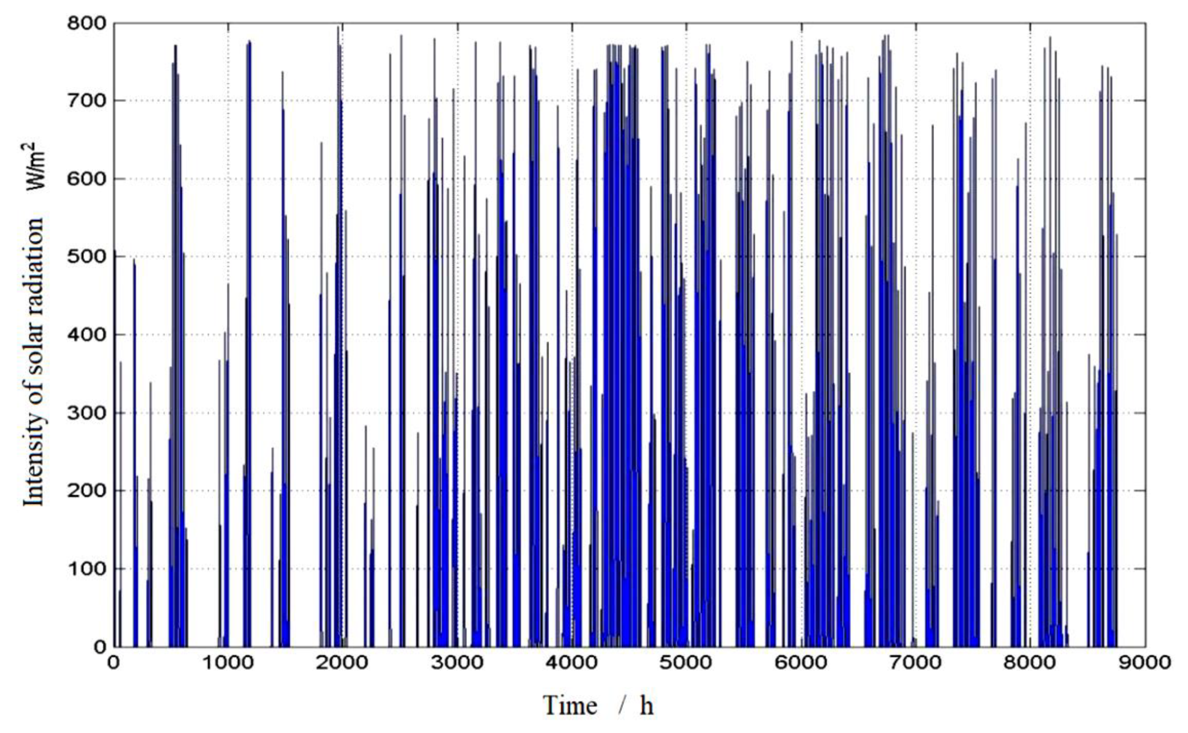
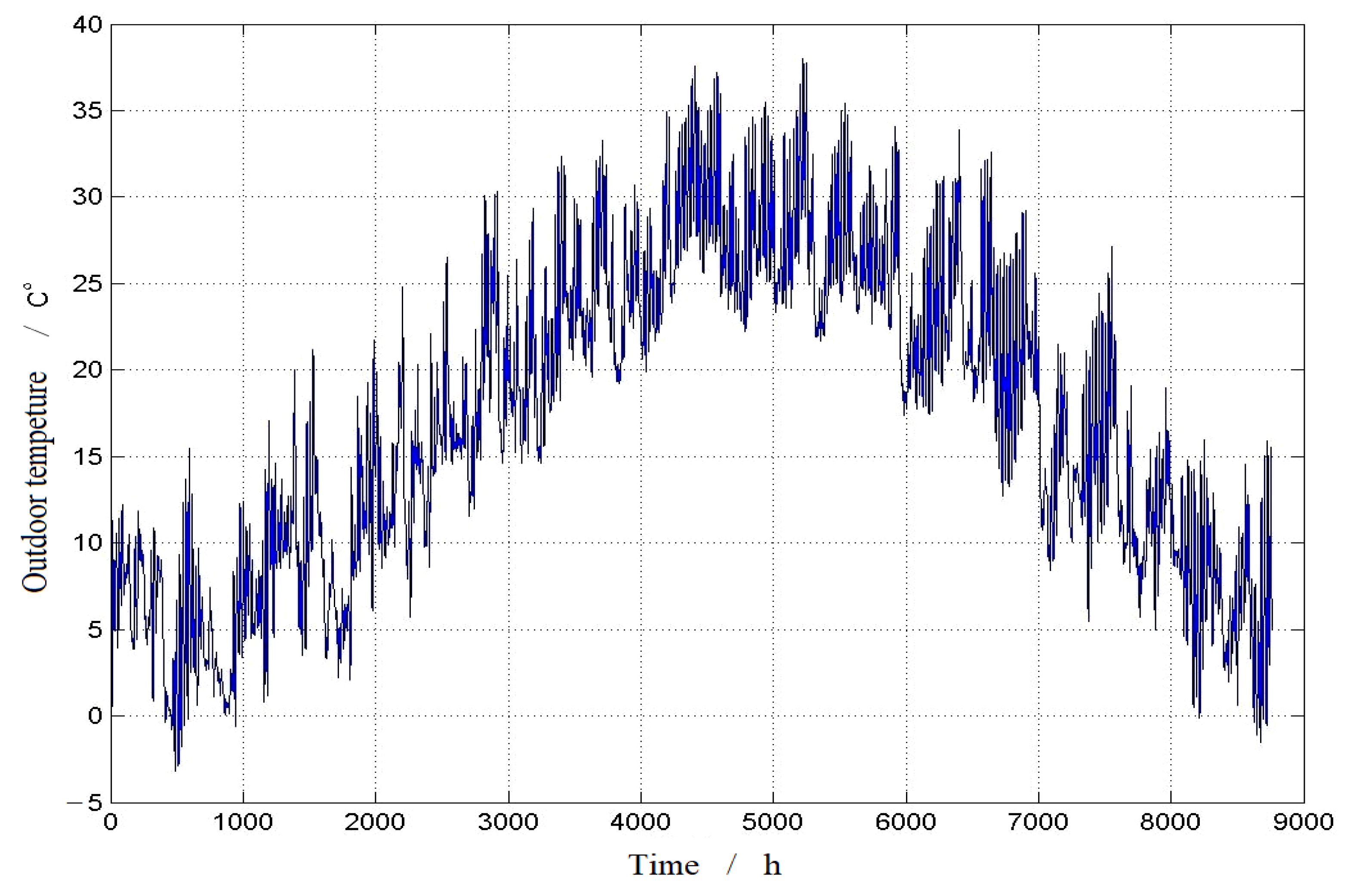
4.1.1. Related Data Selection of the Example

An indoor swimming pool utilizing new energy and renewable energy was selected for our research. The MCS energy structure of the example is shown in Figure 1. The project’s construction area is 1143.20 square meters. The building’s height is 6.61 meters. The average depth of the pool water is 1.20 m, while the length is 30.00 m for the east–west length of the swimming pool and 15 m for the north–south. The roof can host solar photovoltaic panels and flat-plate solar collectors with a maximum area of 372.00 m². The ground-source heat pump can be installed with a maximum capacity of 200.00 kW. The local meteorological conditions need to be considered; thus, the annual hourly solar radiation intensity and annual hourly temperature in the area where the example project is located are shown in Figure 4 and Figure 5, respectively.

The load required for the example was calculated using the EnergyPlus software that is funded by the U.S. Department of Energy’s (DOE) Building Technologies Office (BTO), and managed by the National Renewable Energy Laboratory (NREL), and its specific characteristics are shown in Figure 6. During the heating time of the pool water, the indoor air conditioning is turned on and the temperature is virtually constant. The hourly load required to maintain the constant temperature of the pool water can be considered to be stable, with an average value of 94.73 kW.

Prices for electricity and gas purchased from external power grids were consistent with the local peak and valley electricity prices and municipal gas prices at the calculated time, respectively [33,34], as shown in

Table 1. Peak and valley electricity price and gas price table in Changsha city (Unit: CNY).

Time	0:00–7:00	7:00–9:00	9:00–11:00	11:00–15:00	15:00–19:00	19:00–23:00	23:00–0:00
Electricity price	0.272	0.604	0.809	0.604	0.809	1.087	0.272
Gas price	3.28

.

The related basic data of the equipment during the optimization calculation can be seen in

Table 2. List of equipment-related parameters.

Equipment	Value of Related Parameters		Equipment	Value of Related Parameters
PV	Unit price	CNY 2500/m2	SC	Unit price	CNY 1600/m2
	Maintenance cost coefficient	CNY 0.015/kWh		Maintenance cost coefficient	CNY 0.03/kWh
	Life cycle	20.0 years		Life cycle	30.0 years
GB	Unit price	CNY 900/kW	HE	Unit price	CNY 220/kW
	Maintenance cost coefficient	CNY 0.003/kWh		Maintenance cost coefficient	CNY 0.002/kWh
	Life cycle	20.0 years		Life cycle	20.0 years
ASHP	Unit price	CNY 1200/kW	GSHP	Unit price	CNY 3000/kW
	Maintenance cost coefficient	CNY 0.02/kWh		Maintenance cost coefficient	CNY 0.01/kWh
	Life cycle	20.0 years		Life cycle	20.0 years
ES	Unit price	CNY 1933/kWh	HS	Unit price	CNY 1000/kWh
	Maintenance cost coefficient	CNY 0.026/kWh		Maintenance cost coefficient	CNY 0.013/kWh
	Life cycle	15.0 years		Life cycle	20.0 years
	Charge Efficiency	0.95		Charge Efficiency	0.9
	Discharge Efficiency	0.95		Discharge Efficiency	0.9
	Discharge Rate	0.2		Discharge Rate	0.2
	Loss Rate	0.001		Loss Rate	0.01
	Unit Replacement Cost	CNY 200/kWh		Unit Replacement Cost	CNY 150/kWh

.

4.1.2. Determination of Algorithm Parameters

When using the improved NSGA-III to solve the model, the population number is taken as 200, the iteration time is taken as 1200, and the crossover probability is chosen as 0.9. The population mutation probability is taken as 0.1. The cross-operator distribution index and arithmetic operator distribution index are both taken as 20.

4.2. Optimization Scheme and Result Analysis

4.2.1. Optimization Scheme

In order to reasonably evaluate the optimization results of the bi-level multi-objective model, calculations of single-level programming optimization and bi-level programming operation collaborative optimization for the MCS were carried out according to the improved NSGA-III. Then, the optimization results of the two schemes were compared.

Scheme 1: Multi-objective optimization of single-level programming with the upper programming optimization model;

Scheme 2: Bi-level programming operation collaborative multi-objective optimization with the upper level programming optimization model and lower-level operation optimization model combined.

4.2.2. Optimal Results

The optimal decision results of Scheme 1 are listed in

Table 3. Optimal compromise solution of single-level programming multi-objective optimization of the MCS.

Life Cycle Cost (CNY)	Life Cycle Carbon Emissions (kg)	Energy Efficiency	GB (kW)	PV (m2)	SC (m2)	GSHPh (kW)	GSHPc (kW)	ASHPh (kW)	ASHPc (kW)	HE (kW)	ES (kWh)	HS (kWh)
2,421,400	1,510,000	8.97	178.73	371.45	0.55	199.77	144.24	33.23	5.76	534.91	150.68	19.43

. It can be seen from the table that, under the optimal decision, the three optimization objectives of MCS life cycle planning optimization are the life cycle cost of CNY 2.4214 million, life cycle carbon emissions of 1.51 thousand tons, and life cycle primary energy efficiency of 8.97. Using this optimal solution to determine the rated capacity of each piece of equipment, it can be seen that the capacity of the boiler is moderate. The solar panels with very few solar collectors are mainly photovoltaic power generation panels. By combining the energy storage capacity, energy storage, and energy conversion, the energy storage device could be made full use of to adopt renewable energy for power generation. When focusing on planning optimization in practical engineering, the system design capacity can be reasonably determined by referring to the decision results obtained via the optimization method.

The Pareto optimal solution obtained by Scheme 2 is listed in

Table 4. Optimal compromise solution of bi-level multi-objective optimization of the MCS.

Life Cycle Cost (CNY)	Life Cycle Carbon Emissions (kg)	Energy Efficiency	Total Operating Costs for Lower Objective (CNY)	GB (kW)	PV (m2)	SC (m2)	GSHPh (kW)	GSHPc (kW)	ASHPh (kW)	ASHPc (kW)	HE (kW)	ES (kWh)	HS (kWh)
2,349,200	1,440,000	8.74	2,396,600	126.74	339.72	32.24	199.57	144.37	33.09	3.62	120.13	136.59	36.90

. It can be seen that, under the optimal decision, the three objective values obtained by the upper level programming optimization of Scheme 2 are the life cycle cost of CNY 2.3492 million, life cycle carbon emissions of 1.44 thousand tons, and life cycle primary energy efficiency of 8.74. In the lower model, the total operating cost of the target value obtained by optimization is CNY 2.3966 million when the carbon transaction costs are taken into account. In addition, among the decision variables of Scheme 2, the capacity of the SC, HE, and HS varies greatly. The SC optimization capacity is 58.6 times that of Scheme 1, the HE capacity is of 77% less than that of Scheme 1, and the HS optimization capacity is 1.9 times than that of Scheme 1. Analysis shows that after the optimization under Scheme 2, the utilization of solar energy in terms of thermal energy is increased, reducing the use of heat exchanger equipment with high primary energy consumption, and the multi-energy cascade utilization of the MCS through the adjustment of the heat storage equipment is achieved.

4.3. Further Discussions

In the following section, the objective values and decision variables obtained via the optimal decision scheme under the two schemes are compared.

4.3.1. Comparative Analysis of Optimization Objectives

With the two optimization models, the comparison of the target values based on the optimal decision is shown in Figure 7. For parallel comparison, the operational costs here include only the natural gas and power consumption costs and equipment maintenance costs, under two schemes. It can be seen that the bi-level collaborative optimization model proposed in this study, with multiple constraints based on renewable energy penetration and carbon transaction costs, is superior to the results of single-level multi-objective programming optimization with respect to the life cycle cost and carbon emission objectives; in the former, the total life cycle costs, investment costs, operational costs, and maintenance costs are reduced by 3.0%, 4.0%, 2.3%, and 3.2%, respectively. Life cycle total carbon emissions are decreased by 4.9%. It can be seen, considering the low-carbon operation strategy in the planning optimization, that the low carbon emissions of the multi-energy complementary system replace the high carbon emissions of the purchased energy, on the basis of controlling the economic cost. Thus, the cost optimization and carbon emission results of the bi-level model are superior to the results of single-level multi-objective programming optimization.

4.3.2. Comparative Analysis of Optimization Performance

In the two optimization modes, the comparison of optimization performance based on optimal decisions is shown in Figure 8. The diagram shows that the primary energy efficiency of the bi-level optimization model is 2.6% lower than that of the single-level optimization model, and it is slightly lower than that of the single-level multi-objective optimization model. However, its renewable energy penetration rate is 1.2 times greater than that of the single-level planning optimization. High renewable energy penetration has been achieved to compensate for a slightly lower primary energy efficiency of fossil fuels in the life cycle.

According to the relatively complex bi-level optimization model, the iteration time of the simulation calculation of the model is long, and the average iteration time is 1.7 times that of the single-level multi-objective optimization model. In terms of objective value, the overall optimization results of the bi-level optimization model are indeed better than those of the single-level programming optimization model. However, considering the running time, since the intelligent optimization algorithm needs widespread debugging and system simulation to make the optimal decision, the bi-level optimization calculation is time-consuming, which gives the method a large time limit. Further independent experiments may be carried out in order to obtain more reliable results in terms of the actual engineering optimization. Therefore, in practical engineering applications, the optimization time can be calculated according to the complexity of the project, as well as which optimization scheme is comprehensively considered for system optimization.

4.3.3. Comparative Analysis of Decision Variables

The comparison of decision variables based on the optimal solution under the two optimization strategies is shown in Figure 9. It can be noted, considering the constraint condition of maximum renewable energy penetration and the objective requirement of minimizing the carbon transaction cost, that the overall equipment capacity of the system is reduced after optimization with the bi-level collaborative optimization model. Owing to the limitation of solar panel installation capacity, the photovoltaic solar panel capacity is reduced by 31.73 m², but the flat-panel solar collector capacity is increased by 31.89 m². Analysis shows that the area where the case is located belongs to the hot summer and cold winter area, and the annual sunshine time is long. Under the double-optimization mode, the increase in solar collector area is due to the nature of the example building. Extending to the whole life cycle of the system, the swimming pool needs to increase the amount of heat supply equipment in order to maintain the water temperature. At the same time, the boiler capacity also decreases by 51.99 kW, and the heat storage equipment capacity increases by 17.47 kW—that is, natural gas consumption is reduced, while giving full play to the energy storage characteristics of the MCS. Under the double-layer optimization mode, the heat exchanger capacity decreases further, falling to only 22.5% of the single-level optimization calculation results, and the energy consumption in the life cycle of the system is reduced.

4.4. Comparative Analysis before and after MCS Optimization

The comparison between the single-level multi-objective programming optimization and the bi-level multi-objective collaborative optimization, along with the objective parameters before the optimization, is shown in Figure 10. It can be seen that the investment cost before optimization is low, but it is greatly increased after optimization. Analysis shows that this is because the optimization takes into account the relevant factors of the whole life cycle of the system increasing the renewable energy input during the optimization process and inducing the initial investment cost added.

However, compared with the planning optimization and collaborative optimization, the investment cost of collaborative optimization is slightly lower. The analysis shows that this is because collaborative optimization comprehensively considers the influence of the operation after the completion of the system. The early construction investment is optimized more reasonably in the collaborative process. The improvement of renewable energy input and permeability of engineering are considered from different levels or angles by both optimization models. Extending to the whole life cycle of the MCS, the annual operational cost of the system is significantly reduced after optimization. The change in the system maintenance cost before and after optimization is small. Analysis of this phenomenon indicates that the system maintenance cost is an unavoidable part of the expenditure in the course of the system’s operational life cycle; the optimization has little effect on it. Annual carbon emissions of purchased electricity and natural gas are greatly reduced after optimization, mainly due to the use of renewable energy. Although the purchased electricity carbon emissions from bi-level optimization are slightly higher than those from single-level optimization, the natural gas carbon emissions of bi-level optimization are much lower than those of single-level optimization. Extending to the whole life cycle, the overall carbon emissions of the bi-level optimization are still lower than those of the single-level optimization.

Consequently, it is of great practical significance to improve the investment in renewable energy and maintain a good penetration rate of renewable energy for the realization of the goal of “carbon neutrality”.

5. Conclusions

At present, the traditional energy development model of high consumption and high pollution needs to be abandoned. Seeking a multi-energy complementary comprehensive energy system that can not only meet the changing energy supply structure and user demand, but also promote the efficient utilization of resources in the energy system and low-carbon environmental protection, has become the main direction of future energy development. Consequently, our research on MCS life cycle multi-objective optimization methods was carried out. Based on the bi-level multi-objective optimization theory, a bi-level multi-objective programming operation collaborative optimization model of MCSs was constructed. The upper level takes the minimum life cycle cost, the minimum life cycle carbon emissions, and the maximum primary energy utilization as the optimization objectives. The lower level takes the minimum total operating cost of the whole life cycle as the optimization objective, considering carbon transaction costs and the introduction of high renewable energy penetration as the constraints. At the same time, based on previous research, NSGA-III was improved to enhance the global search ability and convergence speed of the algorithm. According to the case analysis, the constructed bi-level multi-objective collaborative optimization model was solved using the improved NSGA-III.

By comparison with the results of a single-level programming multi-objective optimization model, the following conclusions could be drawn:

• The MCS can determine the rated capacity of a set of systems after obtaining the optimal solution via bi-level optimization or single-level optimization. Overall, the boiler capacity is moderate. The solar panels are mainly photovoltaic power generation panels, and solar energy is very limited. Combined with the energy storage capacity, the MCS makes full use of energy storage devices for energy storage and conversion by relying on renewable energy for power generation;
• Compared with the optimization results of the single-level model, the bi-level optimization considers the constraint conditions of maximum permeability of renewable energy and the objective requirement of minimum carbon transaction cost, reducing the boiler capacity and increasing the flat-plate solar collector capacity. At the same time, the decrease in heat exchanger capacity causes the energy consumption in the system life cycle to decrease to a certain extent;
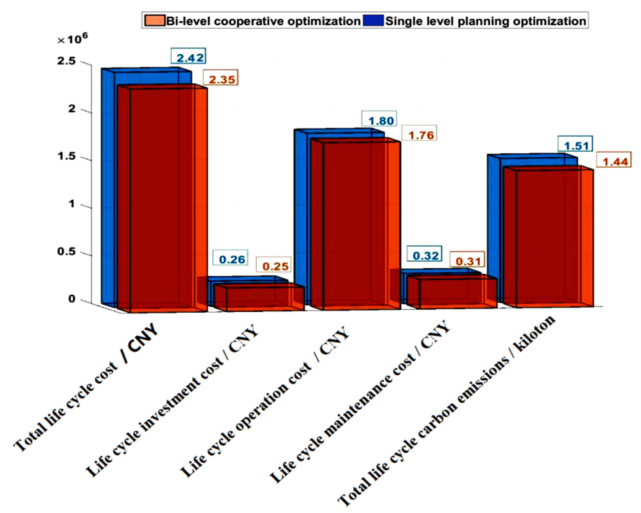
• By comparison with the single-level multi-objective optimization model, the bi-level multi-objective collaborative optimization model proposed in this study can better realize the comprehensive optimization of system planning and operation. Considering the impact of renewable energy penetration constraints and carbon transaction costs, the system’s integrated costs and carbon emissions are better optimized;
• The iteration time of the bi-level multi-objective collaborative optimization model is longer than that of the single-level multi-objective optimization model because of its relatively complex structure. Multiple independent experiments are needed in order to obtain more reliable results in practical engineering optimization; thus, the application of this method has large time limit. In practical engineering applications, it is necessary to consider which optimization scheme should be adopted according to the complexity of the project;
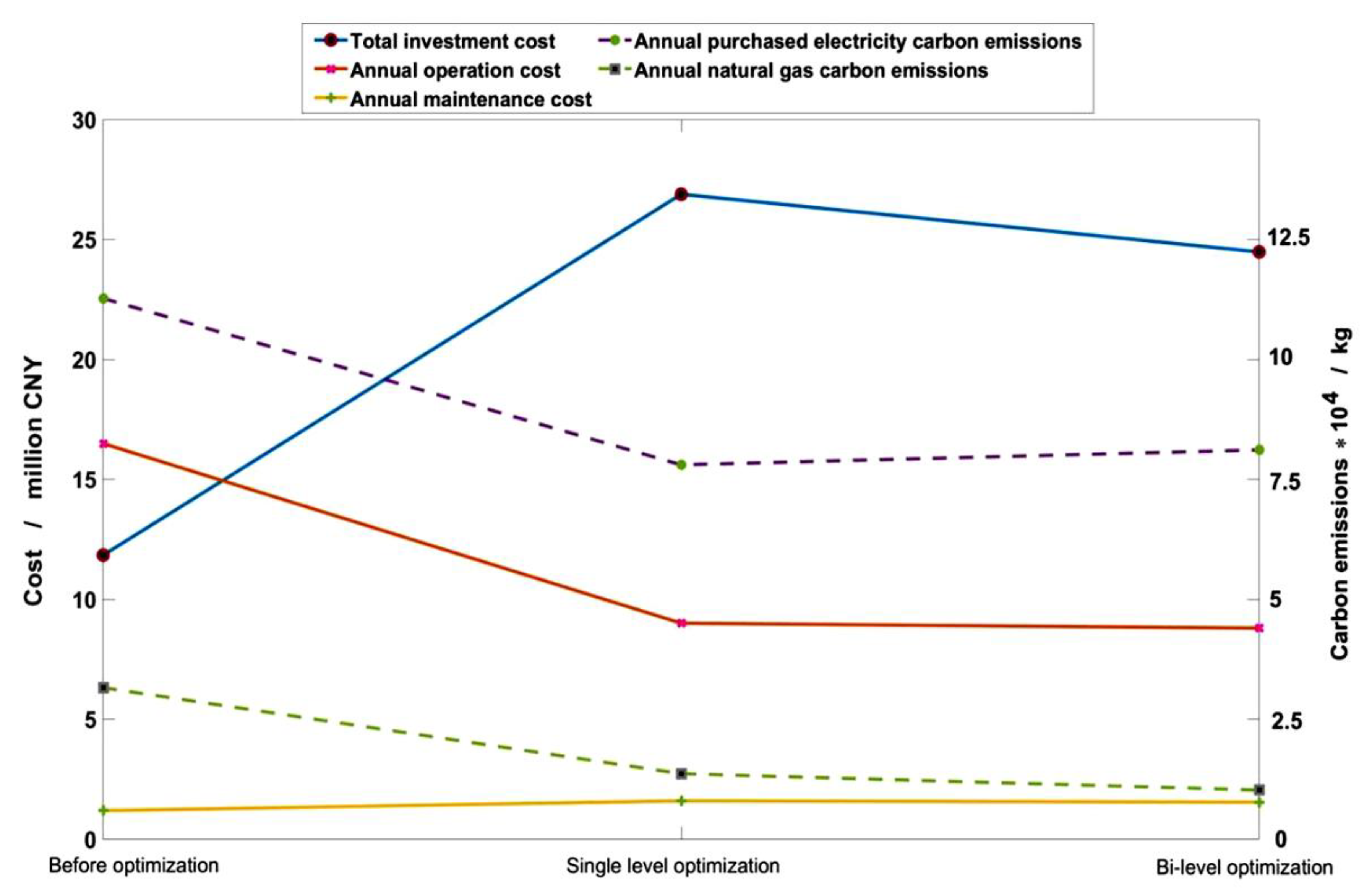
• The optimization results of the two optimization schemes of the case were compared with the cost values before optimization. It can be seen that the investment cost after optimization is higher than that before optimization because of the increase in renewable energy equipment investment during optimization. However, due to the investment of renewable energy, the annual carbon emissions of purchased electricity and natural gas are greatly reduced after optimization. Due to each of the two optimization models taking the impact of the whole life cycle of the MCS into account, the annual operational cost of the optimized system is significantly reduced compared with that before optimization. The system maintenance cost is an unavoidable part of expenditure in the course of the system’s operational life cycle; the optimization has little effect on it. The total cost of the system after optimization is lower than that before optimization, which indicates that the two optimization schemes have good applicability.

The research conclusion of this paper verifies the effectiveness of the proposed bi-level multi-objective collaborative optimization model from the perspective of optimization objectives and optimization performance, showing that it can better realize the comprehensive optimization of system planning and operation. However, this study does not address the specific impact of uncertainty in MCS renewable energy, nor does it consider the interconnection between multiple MCSs with energy storage modules and different characteristics. In addition, total carbon emission value considering the production of the renewable elements of the analyzed system is a question worth exploring. Further research on these issues will be undertaken in the future.

References

1. Huang, Y.; Li, S.; Ding, P.; Zhang, Y.; Yang, K.; Zhang, W. Optimal operation for economic and exergetic objectives of a multiple energy carrier system considering demand response program. Energies 2019, 20, 3995. [Google Scholar] [CrossRef] [Green Version]
2. Wang, Y.L.; Sang, Z.X.; Huang, J.Q.; Yan, J.; Du, Z. Smart grid planning analysis considering multiple renewable energy resources and energy storage systems of user side. IOP Conf. Ser. Earth Environ. Sci. 2021, 634, 012064. [Google Scholar] [CrossRef]
3. Blasio, N.D.; Krishnamoorthy, S.; Kapadia, Z.; Abigail, M.; Rees, S.T. Deploying energy innovation at scale for a low-carbon economy / the private sector role: ENGIE. Innovation 2020, 9, 1–51. Available online: https://www.researchgate.net/publication/344345875 (accessed on 20 April 2021).
4. Mishra, R.; Banerjee, U.; Sekhar, T.; Saha, T.K. Development and implementation of control of stand-alone PMSG-based distributed energy system with variation in input and output parameters. Electr. Power Appl. 2019, 13, 1497–1506. [Google Scholar] [CrossRef]
5. Kabalci, E. Hybrid Renewable Energy Systems and Microgrids; Elsevier: Amsterdam, The Netherlands, 2020. [Google Scholar]
6. Lu, Y.L.; Han, M.X.; Ren, H.B.; Wu, Q. Progress on the design optimization of hybrid distributed energy systems. J. Shanghai Univ. Electr. Power 2018, 03, 229–235. [Google Scholar]
7. Lezama, F.; Soares, J.; Faia, R.; Vale, Z.; Segerstam, J. Bidding in local electricity markets with cascading wholesale market integration. Int. J. Electr. Power Energy Syst. 2021, 131, 107045. [Google Scholar] [CrossRef]
8. Li, K.; Wei, X.G.; Yan, Y.; Zhang, C. Bi-level optimization design strategy for compressed air energy storage of a combined cooling, heating, and power system. J. Energy Storage 2020, 31, 101642. [Google Scholar] [CrossRef]
9. Liu, T.Y.; Dong, G.Z.; Wang, Z.L.; Zeng, X.W.; Zhang, Y.Y.; Yang, J.; Yin, J.H. An optimization approach cconsidering user utility for the PV-storage charging station planning process. Processes 2020, 8, 83. [Google Scholar] [CrossRef] [Green Version]
10. Solanki, B.V.; Raghurajan, A.; Bhattacharya, K.; Canizares, C. Including smart loads for optimal demand response in integrated energy management systems for isolated microgrids. IEEE Trans. Smart Grid 2017, 8, 1739–1748. [Google Scholar] [CrossRef]
11. Zhao, Y.; Peng, K.; Xu, B.; Li, H.; Liu, Y.; Zhang, X. Bilevel Optimal Dispatch Strategy for a Multi-Energy System of Industrial Parks by Considering Integrated Demand Response. Energies 2018, 11, 1942. [Google Scholar] [CrossRef] [Green Version]
12. Barati, F.; Seifi, H.; Sepasian, M.; Nateghi, A.; Shafie-Khah, M.; Catalao, J. Multi-period integrated framework of generation, transmission, and natural gas grid expansion planning for large-scale systems. IEEE Trans. Power Syst. 2015, 30, 2527–2537. [Google Scholar] [CrossRef]
13. Wakui, T.; Hashiguchi, M.; Sawada, K.; Yokoyama, R. Two-stage design optimization based on artificial immune system and mixed-integer linear programming for energy supply networks. Energy 2019, 170, 1228–1248. [Google Scholar] [CrossRef]
14. Liu, C.; Wang, H.; Tang, Y.F.; Wang, Z.Y. Optimization of Multi-energy Complementary Distributed Energy System Based on Comparisons of Two Genetic Opti-mization Algorithms. Processes 2021, 9, 1388. [Google Scholar] [CrossRef]
15. Zhao, L.; Wei, J.X. A nested particle swarm algorithm based on sphere mutation to solve bi-level optimization. Soft Comput. 2019, 23, 11331–11341. [Google Scholar] [CrossRef]
16. Abbassi, M.; Chaabani, A.; Said, L.B.; Absi, N. Bi-level multi-objective combinatorial optimization using reference approximation of the lower level reaction. Procedia Comput. Sci. 2020, 176, 2098–2107. [Google Scholar] [CrossRef]
17. Liu, G.S.; Han, J.Y.; Zhang, J.Z. Exact Penalty Functions for Convex Bi-Level Programming; Plenum Press: New York, NY, USA, 2001. [Google Scholar]
18. Braehe, J.; Mc Gill, J. Mathematical programs with optimization problems in the constraints. Oper. Res. 1973, 21, 37–44. [Google Scholar]
19. Bard, J.F. Practical Bilevel Optimization: Algorithms and Applications; Kluwer Academic Publisher: Dordrecht, The Netherlands, 1998. [Google Scholar]
20. Peng, Z. Distributed Generation Capacity Planning Based on Bi-Level Optimization; Changsha University of Science and Technology: Changsha, China, 2016. [Google Scholar]
21. Guo, J. Research on Active Distribution Network Planning with Distributed Power Access; Harbin Institute of Technology: Harbin, China, 2019. [Google Scholar]
22. Wang, T.; Cui, H.Y.; Wu, G.; Zeng, M. Multi-objective optimization model of regional hybrid energy system compatible with responsive load. Electr. Power Constr. 2018, 39, 30–38. [Google Scholar]
23. Tan, Y.Q. Life Cycle Greenhouse Gas Impacts of Battery Energy Storage Systems in Power System Applications; Nanjing University: Nanjing, China, 2017. [Google Scholar]
24. Zhao, X.; Yang, L.; Qu, X.B.; Yan, W. An improved energy flow calculation method for integrated electricity and natural gas system. Trans. China Electrotech. Soc. 2018, 33, 467–477. [Google Scholar]
25. Wang, S.X.; Zhang, Q.; Wang, H.; Shu, X. Optimal planning method for regional multi-microgrid system with high renewable energy penetration. Electr. Power Autom. Equip. 2018, 38, 33–38, 52. [Google Scholar]
26. Wang, Y.; Zhou, X.; Shi, Y.; Zheng, Z.; Zeng, Q.; Chen, L.; Xiang, B.; Huang, R. Transmission Network Expansion Planning Considering Wind Power and Load Uncertainties Based on Multi-Agent DDQN. Energies 2021, 14, 6073. [Google Scholar] [CrossRef]
27. Wen, L.; Zhang, B.F.; Zhang, E.X.; Tong, B.; Zhao, Y. Optimized planning method for grid-connected multi-energy complementary system. Therm. Power Gener. 2019, 48, 68–72. [Google Scholar]
28. Mehdi, N.; Sergiienko, N.Y.; Erfan, A.; Meysam, M.N.; Davide, A.G.; Bradley, A.; Markus, W. A New Bi-Level Optimisation Framework for Optimising a Multi-Mode Wave Energy Converter Design: A Case Study for the Marettimo Island, Mediterranean Sea. Energies 2020, 13, 5498. [Google Scholar]
29. Sinha, A.; Malo, P.; Deb, K. A Review on Bilevel Optimization: From Classical to Evolutionary Approaches and Applications. IEEE Trans. Evol. Comput. 2018, 2, 276–295. [Google Scholar] [CrossRef]
30. Deb, K.; Jain, H. An evolutionary many-objective optimization algorithm using reference-point-based non-dominated sorting approach, part I: Solving problems with box constraints. IEEE Trans. Evol. Comput. 2014, 18, 577–601. [Google Scholar] [CrossRef]
31. Xiao, B.Q.; Liu, Y.; Dai, G.M. Improved NSGA-II algorithm and its application in optimization of satellite constellation. Comput. Eng. Appl. 2012, 48, 47–53. [Google Scholar]
32. Brown, P.D.; Lopes, J.; Matos, M.A. Optimization of pumped storage capacity in an isolated power system with large renewable penetration. IEEE Trans. Power Syst. 2008, 23, 523–531. [Google Scholar] [CrossRef]
33. Hunan Province Electricity Rate Price List in 2020 [EB/OL]. Available online: http://m.cs.bendibao.com/news/63055.shtm (accessed on 11 January 2021).
34. Pipeline Gas Charges [EB/OL]. Available online: http://www.cs95158.cn/contents/68/1594.html (accessed on 15 February 2021).
Figure 1. Energy supply structure of the final MCS.
Energies 14 07930 g001
Figure 2. Calculation process of the bi-level multi-objective collaborative optimization model.
Energies 14 07930 g002
Figure 3. Schematic flow diagram of the improved NSGA-III.
Energies 14 07930 g003
Figure 4. Annual hourly solar radiation intensity.
Energies 14 07930 g004
Figure 5. Annual hourly outdoor ambient temperature.
Energies 14 07930 g005
Figure 6. Annual hourly terminal load.
Energies 14 07930 g006
Figure 7. Comparison of objective cost and carbon emission vales under optimal solution strategies.
Energies 14 07930 g007
Figure 8. Comparison of iteration time and energy efficiency.
Energies 14 07930 g008
Figure 9. Comparison of decision variables under optimal decisions.
Energies 14 07930 g009
Figure 10. Comparison of before and after optimization of the example MCS.
Energies 14 07930 g010