
Stability Analysis of Grid-Forming MMC-HVDC Transmission Connected to Legacy Power Systems

 ,
,  , ,
, ,  , and
, and
Abstract
:1. Introduction
2. Grid-Forming and Grid-Following Control Strategies for Modular Multilevel Converters
2.1. Classification of Control Strategies for Power Converters
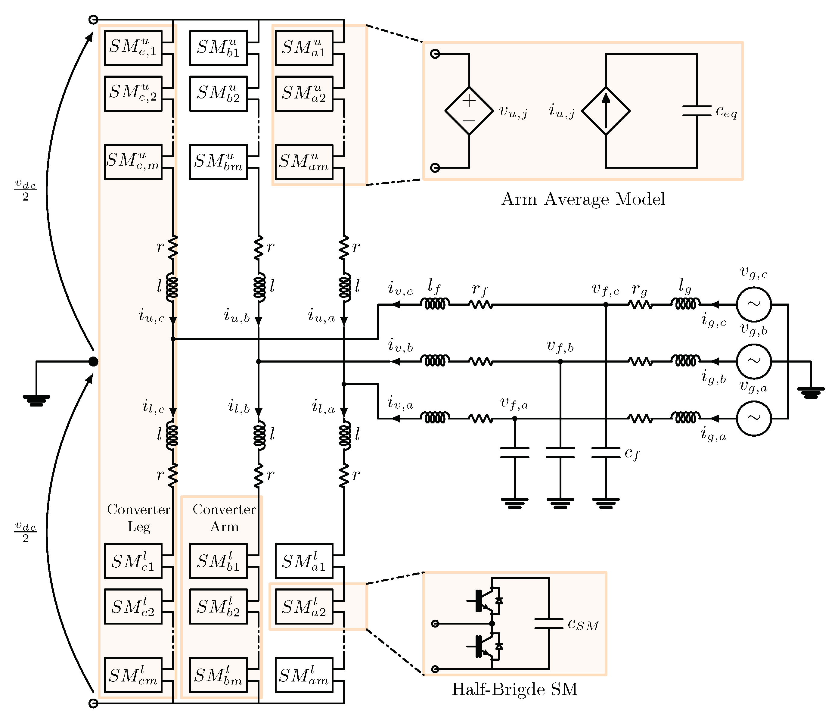
2.2. Modular Multilevel Converter Model
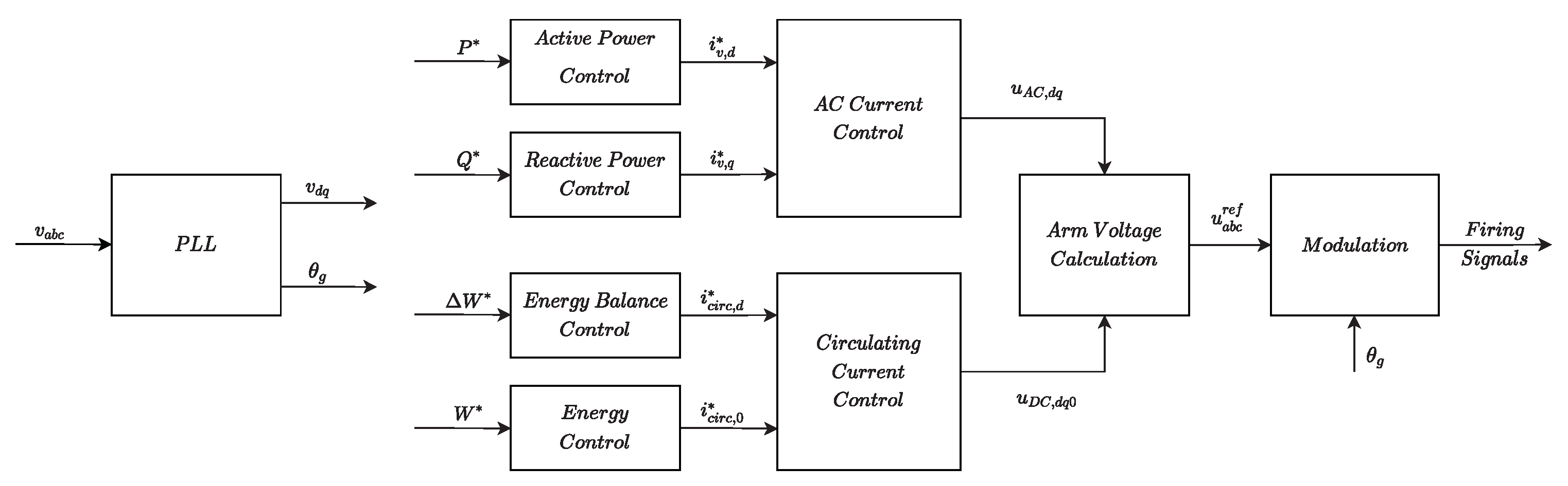
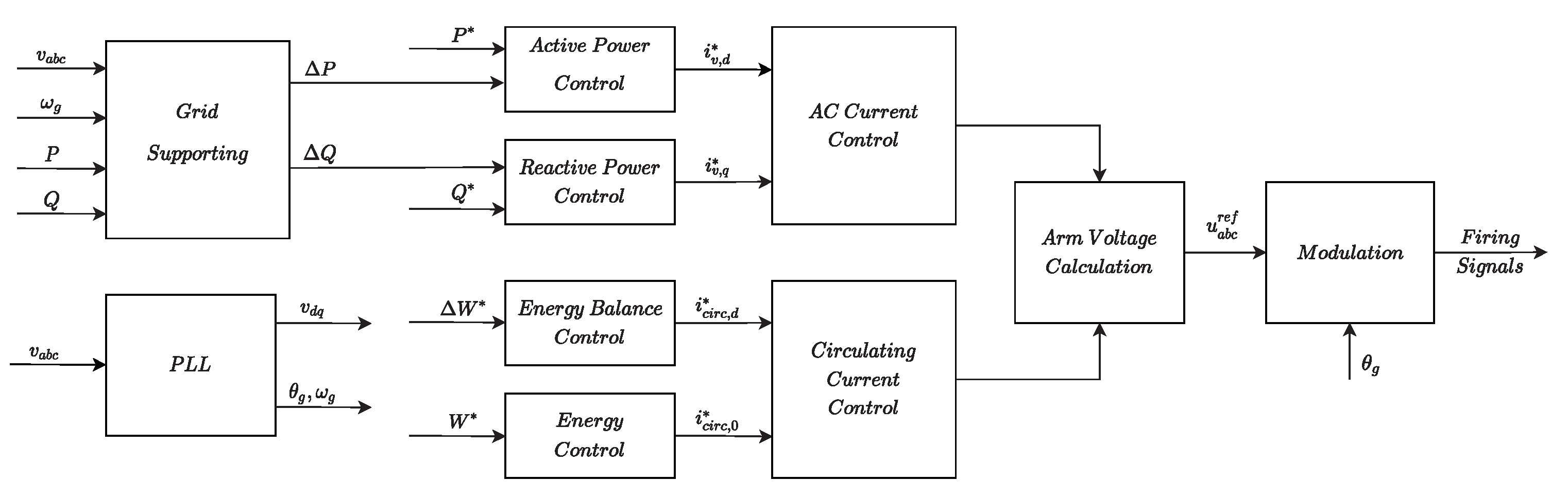
2.3. Grid Following (GFL)
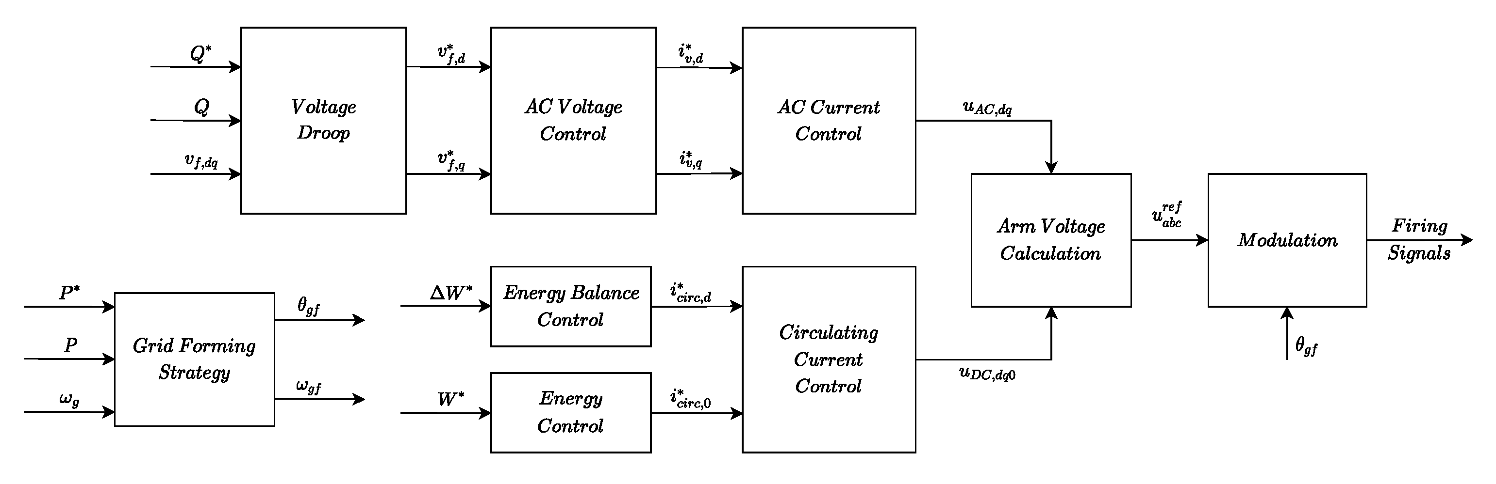
2.4. Grid Forming (GFM)
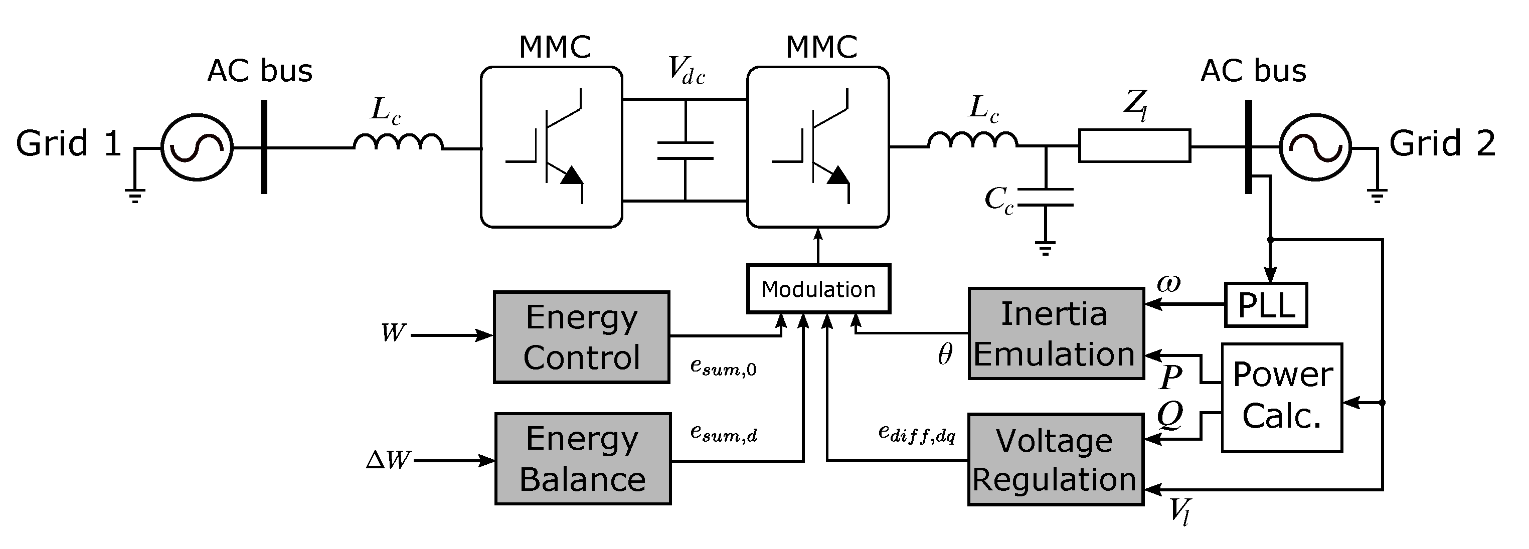
2.4.1. Virtual Synchronous Machine
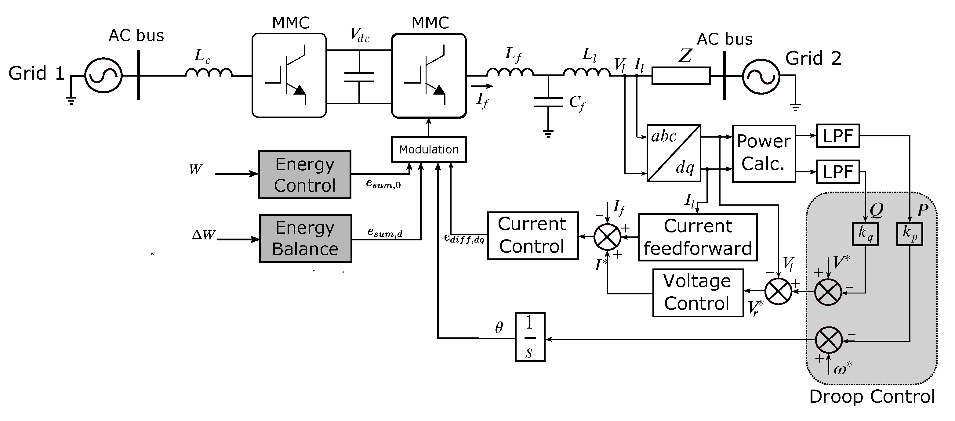
2.4.2. Droop-Based Topology
3. Modeling of a Multi-Machine, Multi-Converter Power System
3.1. Generators and Converters Models
3.2. Center-of-Inertia Formulation of a Multi-Machine, Multi-GFM Converter Power System
4. Lyapunov-Based Stability Analysis Using Energy Functions
4.1. Energy Functions for Synchronous Generators and GFM Converters
4.2. Multi-Machine, Multi-GFM Converter System Stability Analysis
5. Simulations and Results
- Scenario 1: Both MMC-HVDCs follow the VSM control strategy;
- Scenario 2: Both MMC-HVDCs follow the droop control strategy;
- Scenario 3: MMC-HVDC-1 follows the VSM control strategy, and MMC-HVDC-2 follows the droop control strategy.
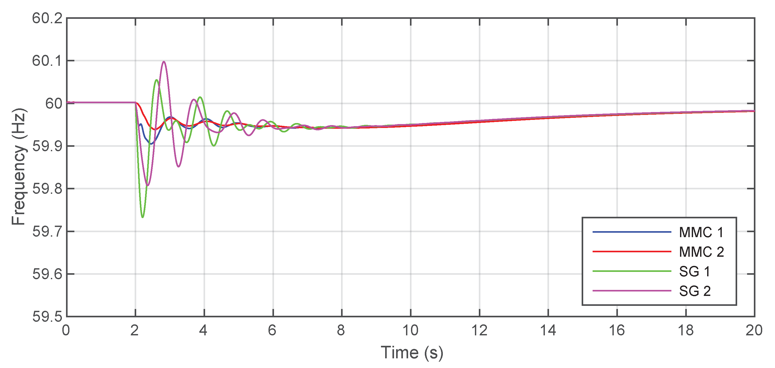
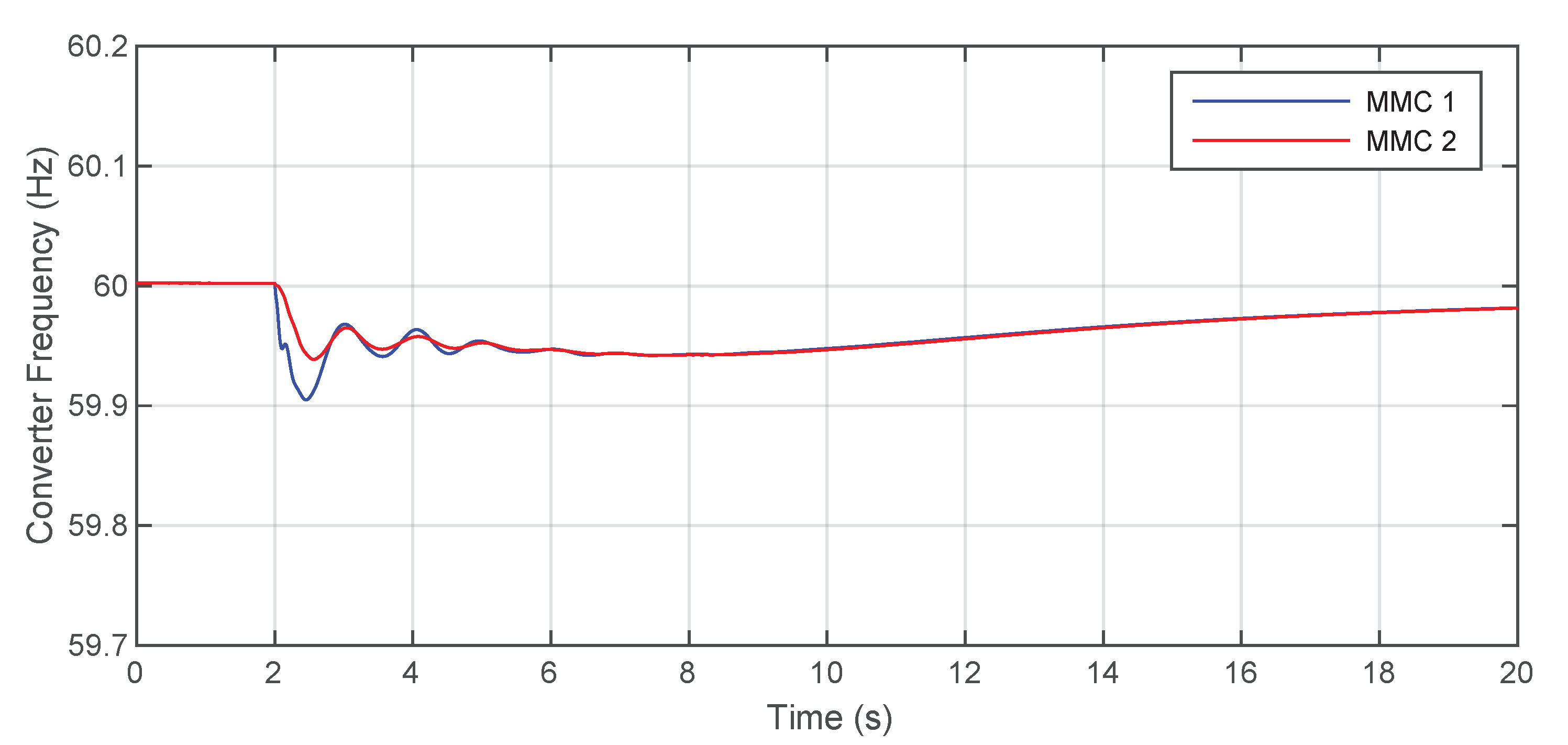
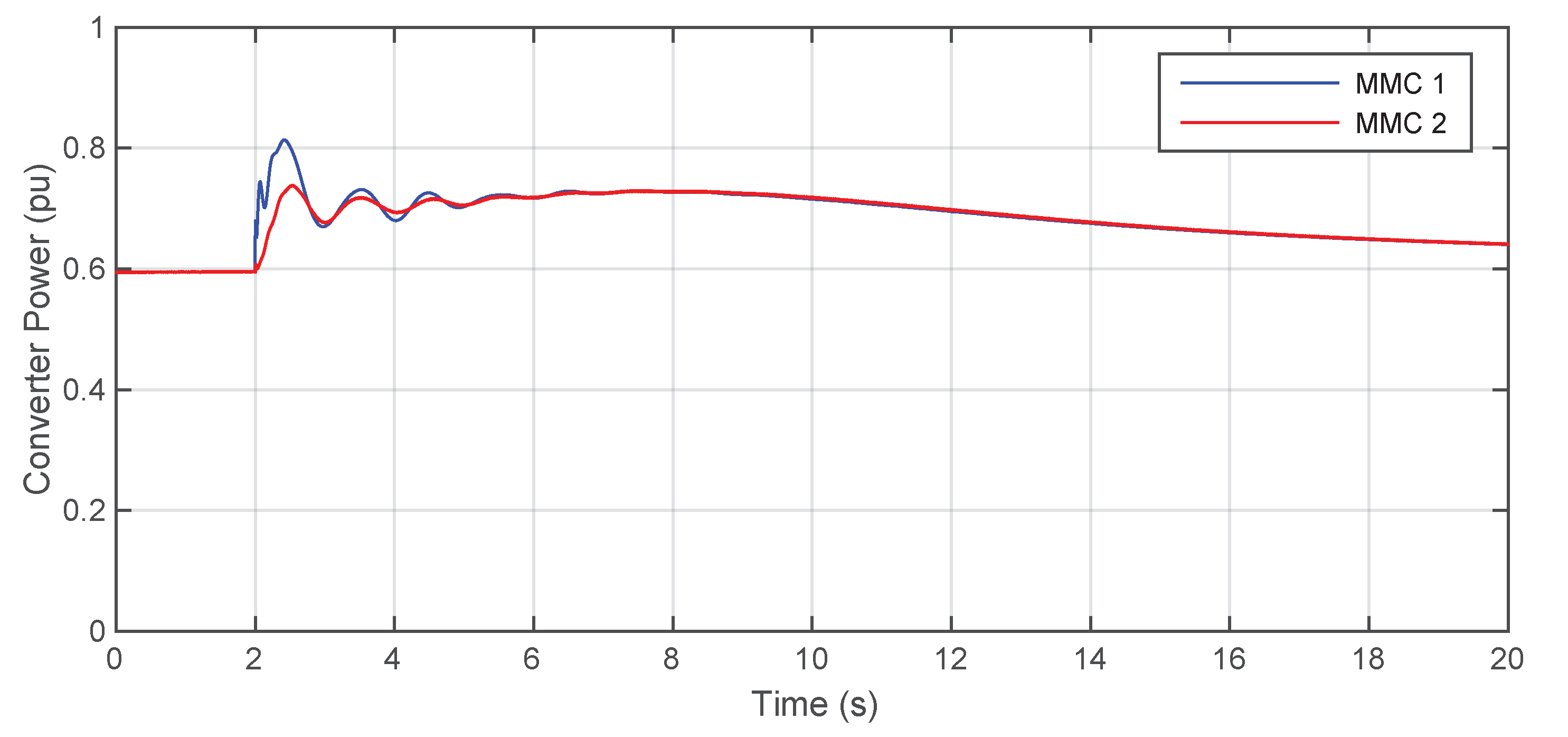
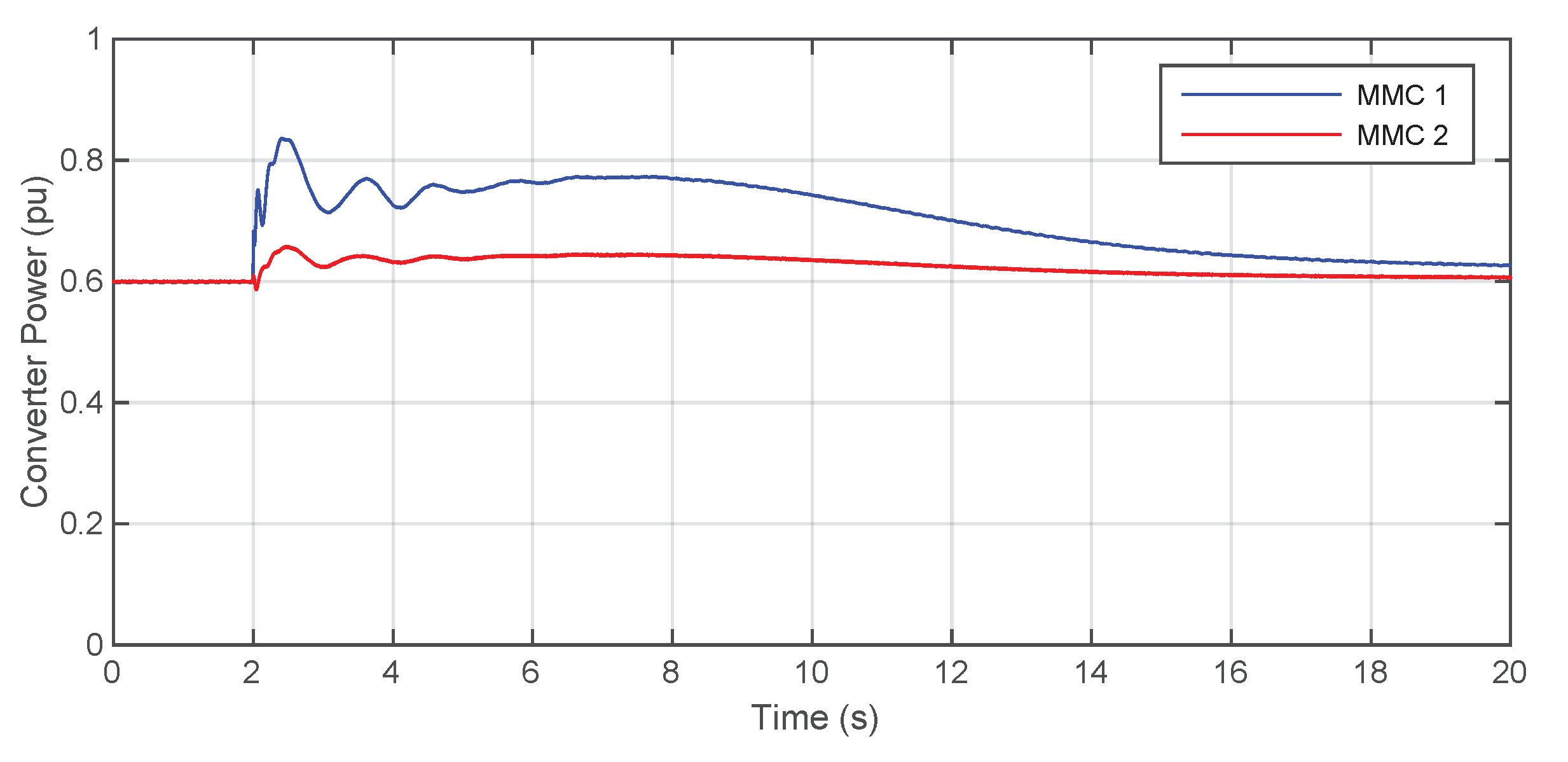
5.1. First Scenario: Two VSM-GFM Converters
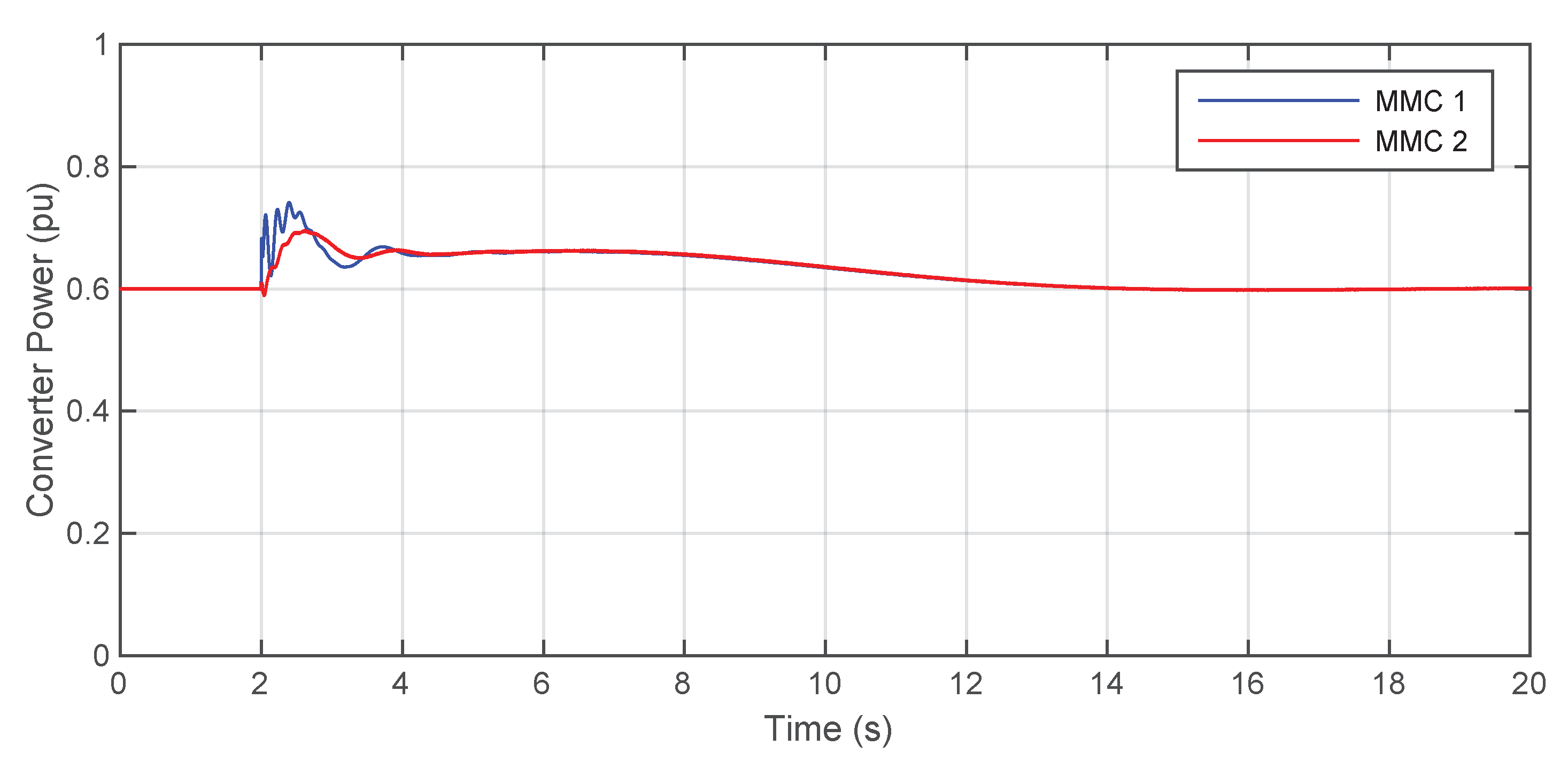
5.2. Second Scenario: Two Droop GFM Converters
5.3. Third Scenario: One VSM and One Droop GFM Converter
5.4. The Role of Virtual Inertia
6. Conclusions
Author Contributions
Funding
Conflicts of Interest
Abbreviations
| MMC | Modular multilevel converter |
| HVDC | High-voltage direct-current |
| DC | Direct durrent |
| AC | Alternating current |
| VSM | Virtual synchronous machine |
| PCC | Point of common coupling |
| GFM | Grid forming |
| GFL | Grid following |
| PLL | Phase-locked loop |
| VSC | Voltage source converter |
| LPF | Low-pass filter |
| PI | Proportional-integral controller |
| ROCOF | Rate of change of frequency |
| PWM | Pulse width modulation |
| SG | Synchronous generator |
References
- Liang, J.; Jing, T.; Gomis-Bellmunt, O.; Ekanayake, J.; Jenkins, N. Operation and control of multiterminal HVDC transmission for offshore wind farms. IEEE Trans. Power Deliv. 2011, 26, 2596–2604. [Google Scholar] [CrossRef]
- Gonzalez-Torres, J.C.; Damm, G.; Costan, V.; Benchaib, A.; Lamnabhi-Lagarrigue, F. Transient stability of power systems with embedded VSC-HVDC links: Stability margins analysis and control. IET Gener. Transm. Distrib. 2020, 14, 3377–3388. [Google Scholar] [CrossRef]
- Gonzalez-Torres, J.C.; Damm, G.; Costan, V.; Benchaib, A.; Lamnabhi-Lagarrigue, F. A novel distributed supplementary control of Multi-Terminal VSC-HVDC grids for rotor angle stability enhancement of AC/DC systems. IEEE Trans. Power Syst. 2020, 36, 623–634. [Google Scholar] [CrossRef]
- Milano, F.; Dörfler, F.; Hug, G.; Hill, D.J.; Verbič, G. Foundations and challenges of low-inertia systems. In Proceedings of the 2018 Power Systems Computation Conference (PSCC), Dublin, Ireland, 11–15 June 2018; IEEE: Piscataway, NJ, USA, 2018; pp. 1–25. [Google Scholar]
- Meegahapola, L.; Sguarezi, A.; Bryant, J.S.; Gu, M.; Conde, D.E.R.; Cunha, R. Power system stability with power-electronic converter interfaced renewable power generation: Present issues and future trends. Energies 2020, 13, 3441. [Google Scholar] [CrossRef]
- Lasseter, R.H.; Chen, Z.; Pattabiraman, D. Grid-forming inverters: A critical asset for the power grid. IEEE J. Emerg. Sel. Top. Power Electron. 2019, 8, 925–935. [Google Scholar] [CrossRef]
- 9 August 2019 Power Outage Report; Technical Report; OFGEM: UK, 2019. Available online: https://www.ofgem.gov.uk/sites/default/files/docs/9_august_2019_power_outage_report.pdf (accessed on 15 October 2021).
- Oni, O.E.; Davidson, I.E.; Mbangula, K.N. A review of LCC-HVDC and VSC-HVDC technologies and applications. In Proceedings of the 2016 IEEE 16th International Conference on Environment and Electrical Engineering (EEEIC), Florence, Italy, 7–10 June 2016; IEEE: Piscataway, NJ, USA, 2016; pp. 1–7. [Google Scholar]
- Jovcic, D. High Voltage Direct Current Transmission: Converters, Systems and DC Grids; John Wiley & Sons: Hoboken, NJ, USA, 2019. [Google Scholar]
- Lesnicar, A.; Marquardt, R. An innovative modular multilevel converter topology suitable for a wide power range. In Proceedings of the 2003 IEEE Bologna Power Tech Conference Proceedings, Bologna, Italy, 23–26 June 2003; IEEE: Piscataway, NJ, USA, 2003; Volume 3, p. 6. [Google Scholar]
- Marquardt, R. Modular Multilevel Converter: An universal concept for HVDC-Networks and extended DC-Bus-applications. In Proceedings of the 2010 International Power Electronics Conference-ECCE ASIA, Sapporo, Japan, 21–24 June 2010; IEEE: Piscataway, NJ, USA, 2010; pp. 502–507. [Google Scholar]
- Glinka, M.; Marquardt, R. A new AC/AC multilevel converter family. IEEE Trans. Ind. Electron. 2005, 52, 662–669. [Google Scholar] [CrossRef]
- Peralta, J.; Saad, H.; Dennetière, S.; Mahseredjian, J.; Nguefeu, S. Detailed and averaged models for a 401-level MMC–HVDC system. IEEE Trans. Power Deliv. 2012, 27, 1501–1508. [Google Scholar] [CrossRef]
- Van Hertem, D.; Gomis-Bellmunt, O.; Liang, J. HVDC Grids: For Offshore and Supergrid of the Future; John Wiley & Sons: Hoboken, NJ, USA, 2016. [Google Scholar]
- Hatziargyriou, N.; Milanovic, J.; Rahmann, C.; Ajjarapu, V.; Canizares, C.; Erlich, I.; Hill, D.; Hiskens, I.; Kamwa, I.; Pal, B.; et al. Definition and classification of power system stability revisited & extended. IEEE Trans. Power Syst. 2020, 36, 3271–3281. [Google Scholar]
- Teodorescu, R.; Liserre, M.; Rodriguez, P. Grid Converters for Photovoltaic and Wind Power Systems; John Wiley & Sons: Hoboken, NJ, USA, 2011; Volume 29. [Google Scholar]
- Yazdani, A.; Iravani, R. Voltage-Sourced Converters in Power Systems: Modeling, Control, and Applications; John Wiley & Sons: Hoboken, NJ, USA, 2010. [Google Scholar]
- Ali, Z.; Christofides, N.; Hadjidemetriou, L.; Kyriakides, E.; Yang, Y.; Blaabjerg, F. Three-phase phase-locked loop synchronization algorithms for grid-connected renewable energy systems: A review. Renew. Sustain. Energy Rev. 2018, 90, 434–452. [Google Scholar] [CrossRef] [Green Version]
- Collados-Rodriguez, C.; Cheah-Mane, M.; Prieto-Araujo, E.; Gomis-Bellmunt, O. Stability analysis of systems with high VSC penetration: Where Is the limit? IEEE Trans. Power Deliv. 2019, 35, 2021–2031. [Google Scholar] [CrossRef]
- Matevosyan, J.; Badrzadeh, B.; Prevost, T.; Quitmann, E.; Ramasubramanian, D.; Urdal, H.; Achilles, S.; MacDowell, J.; Huang, S.H.; Vital, V.; et al. Grid-forming inverters: Are they the key for high renewable penetration? IEEE Power Energy Mag. 2019, 17, 89–98. [Google Scholar] [CrossRef]
- Unruh, P.; Nuschke, M.; Strauß, P.; Welck, F. Overview on grid-forming inverter control methods. Energies 2020, 13, 2589. [Google Scholar] [CrossRef]
- D’Arco, S.; Suul, J.A.; Fosso, O.B. Small-signal modeling and parametric sensitivity of a virtual synchronous machine in islanded operation. Int. J. Electr. Power Energy Syst. 2015, 72, 3–15. [Google Scholar] [CrossRef] [Green Version]
- D’Arco, S.; Suul, J.A.; Fosso, O.B. A Virtual Synchronous Machine implementation for distributed control of power converters in SmartGrids. Electr. Power Syst. Res. 2015, 122, 180–197. [Google Scholar] [CrossRef]
- Zhong, Q.C.; Weiss, G. Synchronverters: Inverters that mimic synchronous generators. IEEE Trans. Ind. Electron. 2010, 58, 1259–1267. [Google Scholar] [CrossRef]
- Zhong, Q.C.; Ma, Z.; Ming, W.L.; Konstantopoulos, G.C. Grid-friendly wind power systems based on the synchronverter technology. Energy Convers. Manag. 2015, 89, 719–726. [Google Scholar] [CrossRef]
- Aouini, R.; Marinescu, B.; Kilani, K.B.; Elleuch, M. Synchronverter-based emulation and control of HVDC transmission. IEEE Trans. Power Syst. 2015, 31, 278–286. [Google Scholar] [CrossRef]
- Hart, P.J.; Lasseter, R.H.; Jahns, T.M. Coherency identification and aggregation in grid-forming droop-controlled inverter networks. IEEE Trans. Ind. Appl. 2019, 55, 2219–2231. [Google Scholar] [CrossRef]
- Rokrok, E.; Qoria, T.; Bruyere, A.; Francois, B.; Zhang, H.; Belhaouane, M.; Guillaud, X. Impact of grid-forming control on the internal energy of a modular multilevel converter. In Proceedings of the 2020 22nd European Conference on Power Electronics and Applications (EPE’20 ECCE Europe), Lyon, France, 7–11 September 2020; IEEE: Piscataway, NJ, USA, 2020; pp. 1–10. [Google Scholar]
- Guo, J.; Chen, Y.; Liao, S.; Wu, W.; Wang, X.; Guerrero, J.M. Low-Frequency Oscillation Analysis of VSMs-Based VSC-HVDC Systems Based on the Five-Dimension Impedance Stability Criterion. IEEE Trans. Ind. Electron. 2021. [Google Scholar] [CrossRef]
- Rokrok, E.; Qoria, T.; Bruyere, A.; Francois, B.; Guillaud, X. Classification and dynamic assessment of droop-based grid-forming control schemes: Application in HVDC systems. Electr. Power Syst. Res. 2020, 189, 106765. [Google Scholar] [CrossRef]
- Raza, M.; Peñalba, M.A.; Gomis-Bellmunt, O. Short circuit analysis of an offshore AC network having multiple grid forming VSC-HVDC links. Int. J. Electr. Power Energy Syst. 2018, 102, 364–380. [Google Scholar] [CrossRef]
- Tian, S.; Campos-Gaona, D.; A Lacerda, V.; Torres-Olguin, R.E.; Anaya-Lara, O. Novel control approach for a hybrid grid-forming HVDC offshore transmission system. Energies 2020, 13, 1681. [Google Scholar] [CrossRef] [Green Version]
- Sánchez-Sánchez, E.; Prieto-Araujo, E.; Gomis-Bellmunt, O. The role of the internal energy in MMCs operating in grid-forming mode. IEEE J. Emerg. Sel. Top. Power Electron. 2019, 8, 949–962. [Google Scholar] [CrossRef]
- Fu, X.; Sun, J.; Huang, M.; Tian, Z.; Yan, H.; Iu, H.H.C.; Hu, P.; Zha, X. Large-signal stability of grid-forming and grid-following controls in voltage source converter: A comparative study. IEEE Trans. Power Electron. 2020, 36, 7832–7840. [Google Scholar] [CrossRef]
- Pan, D.; Wang, X.; Liu, F.; Shi, R. Transient stability of voltage-source converters with grid-forming control: A design-oriented study. IEEE J. Emerg. Sel. Top. Power Electron. 2019, 8, 1019–1033. [Google Scholar] [CrossRef]
- He, X.; Geng, H. Transient Stability of Power Systems Dominated by Different Types of Grid-Forming Devices. arXiv 2021, arXiv:2104.10849. [Google Scholar] [CrossRef]
- Shuai, Z.; Shen, C.; Liu, X.; Li, Z.; Shen, Z.J. Transient angle stability of virtual synchronous generators using Lyapunov’s direct method. IEEE Trans. Smart Grid 2018, 10, 4648–4661. [Google Scholar] [CrossRef]
- Ackermann, T.; Ellis, A.; Fortmann, J.; Matevosyan, J.; Muljadi, E.; Piwko, R.; Pourbeik, P.; Quitmann, E.; Sorensen, P.; Urdal, H.; et al. Code shift: Grid specifications and dynamic wind turbine models. IEEE Power Energy Mag. 2013, 11, 72–82. [Google Scholar] [CrossRef]
- Vandoorn, T.; De Kooning, J.; Meersman, B.; Vandevelde, L. Review of primary control strategies for islanded microgrids with power-electronic interfaces. Renew. Sustain. Energy Rev. 2013, 19, 613–628. [Google Scholar] [CrossRef]
- Han, H.; Hou, X.; Yang, J.; Wu, J.; Su, M.; Guerrero, J.M. Review of power sharing control strategies for islanding operation of AC microgrids. IEEE Trans. Smart Grid 2015, 7, 200–215. [Google Scholar] [CrossRef] [Green Version]
- Rocabert, J.; Luna, A.; Blaabjerg, F.; Rodriguez, P. Control of power converters in AC microgrids. IEEE Trans. Power Electron. 2012, 27, 4734–4749. [Google Scholar] [CrossRef]
- Debnath, S.; Qin, J.; Bahrani, B.; Saeedifard, M.; Barbosa, P. Operation, control, and applications of the modular multilevel converter: A review. IEEE Trans. Power Electron. 2014, 30, 37–53. [Google Scholar] [CrossRef]
- Raju, M.N.; Sreedevi, J.; Mandi, R.P.; Meera, K. Modular multilevel converters technology: A comprehensive study on its topologies, modelling, control and applications. IET Power Electron. 2019, 12, 149–169. [Google Scholar] [CrossRef]
- Antonopoulos, A.; Angquist, L.; Nee, H.P. On dynamics and voltage control of the modular multilevel converter. In Proceedings of the 2009 13th European Conference on Power Electronics and Applications, Barcelona, Spain, 8–10 September 2009; IEEE: Piscataway, NJ, USA, 2009; pp. 1–10. [Google Scholar]
- Saad, H.; Guillaud, X.; Mahseredjian, J.; Dennetiere, S.; Nguefeu, S. MMC capacitor voltage decoupling and balancing controls. IEEE Trans. Power Deliv. 2014, 30, 704–712. [Google Scholar] [CrossRef]
- Sharifabadi, K.; Harnefors, L.; Nee, H.P.; Norrga, S.; Teodorescu, R. Design, Control, and Application of Modular Multilevel Converters for HVDC Transmission Systems; John Wiley & Sons: Hoboken, NJ, USA, 2016. [Google Scholar]
- Bergna, G.; Berne, E.; Egrot, P.; Lefranc, P.; Arzande, A.; Vannier, J.C.; Molinas, M. An energy-based controller for HVDC modular multilevel converter in decoupled double synchronous reference frame for voltage oscillation reduction. IEEE Trans. Ind. Electron. 2012, 60, 2360–2371. [Google Scholar] [CrossRef]
- Bergna-Diaz, G.; Suul, J.A.; D’Arco, S. Energy-based state-space representation of modular multilevel converters with a constant equilibrium point in steady-state operation. IEEE Trans. Power Electron. 2017, 33, 4832–4851. [Google Scholar] [CrossRef] [Green Version]
- Bergna-Diaz, G.; Freytes, J.; Guillaud, X.; D’Arco, S.; Suul, J.A. Generalized voltage-based state-space modeling of modular multilevel converters with constant equilibrium in steady state. IEEE J. Emerg. Sel. Top. Power Electron. 2018, 6, 707–725. [Google Scholar] [CrossRef] [Green Version]
- Prieto-Araujo, E.; Junyent-Ferré, A.; Collados-Rodríguez, C.; Clariana-Colet, G.; Gomis-Bellmunt, O. Control design of Modular Multilevel Converters in normal and AC fault conditions for HVDC grids. Electr. Power Syst. Res. 2017, 152, 424–437. [Google Scholar] [CrossRef] [Green Version]
- Dadjo Tavakoli, S.; Prieto-Araujo, E.; Sánchez-Sánchez, E.; Gomis-Bellmunt, O. Interaction assessment and stability analysis of the MMC-based VSC-HVDC link. Energies 2020, 13, 2075. [Google Scholar] [CrossRef] [Green Version]
- Vatani, M.; Hovd, M.; Saeedifard, M. Control of the modular multilevel converter based on a discrete-time bilinear model using the sum of squares decomposition method. IEEE Trans. Power Deliv. 2015, 30, 2179–2188. [Google Scholar] [CrossRef]
- de Oliveira, G.C.; Damm, G.; Monaro, R.M.; Lourenco, L.F.; Carrizosa, M.J.; Lamnabhi-Lagarrigue, F. Nonlinear control for modular multilevel converters with enhanced stability region and arbitrary closed loop dynamics. Int. J. Electr. Power Energy Syst. 2021, 126, 106590. [Google Scholar] [CrossRef]
- Antonopoulos, A.; Ängquist, L.; Harnefors, L.; Ilves, K.; Nee, H.P. Global asymptotic stability of modular multilevel converters. IEEE Trans. Ind. Electron. 2013, 61, 603–612. [Google Scholar] [CrossRef]
- Harnefors, L.; Antonopoulos, A.; Ilves, K.; Nee, H.P. Global asymptotic stability of current-controlled modular multilevel converters. IEEE Trans. Power Electron. 2014, 30, 249–258. [Google Scholar] [CrossRef]
- Saad, H.; Peralta, J.; Dennetiere, S.; Mahseredjian, J.; Jatskevich, J.; Martinez, J.; Davoudi, A.; Saeedifard, M.; Sood, V.; Wang, X.; et al. Dynamic averaged and simplified models for MMC-based HVDC transmission systems. IEEE Trans. Power Deliv. 2013, 28, 1723–1730. [Google Scholar] [CrossRef]
- Sánchez-Sánchez, E.; Prieto-Araujo, E.; Junyent-Ferré, A.; Gomis-Bellmunt, O. Analysis of MMC energy-based control structures for VSC-HVDC links. IEEE J. Emerg. Sel. Top. Power Electron. 2018, 6, 1065–1076. [Google Scholar] [CrossRef] [Green Version]
- Miller, N.; Lew, D.; Piwko, R. Technology capabilities for fast frequency response. GE Energy Consult. Tech. Rep. 2017, 3, 10–60. [Google Scholar]
- Meegahapola, L.; Mancarella, P.; Flynn, D.; Moreno, R. Power system stability in the transition to a low carbon grid: A techno-economic perspective on challenges and opportunities. Wiley Interdiscip. Rev. Energy Environ. 2021, 10, e399. [Google Scholar] [CrossRef]
- Kundur, P. Power System Stability and Control. Stab. Control; McGraw-Hill: New York, NY, USA, 1994. [Google Scholar]
- Rebours, Y.G.; Kirschen, D.S.; Trotignon, M.; Rossignol, S. A survey of frequency and voltage control ancillary services—Part I: Technical features. IEEE Trans. Power Syst. 2007, 22, 350–357. [Google Scholar] [CrossRef]
- Lee, J.O.; Kim, Y.S. Frequency and State-of-Charge Restoration Method in a Secondary Control of an Islanded Microgrid without Communication. Appl. Sci. 2020, 10, 1558. [Google Scholar] [CrossRef] [Green Version]
- Dohler, J.S.; de Almeida, P.M.; de Oliveira, J.G. Droop Control for Power Sharing and Voltage and Frequency Regulation in Parallel Distributed Generations on AC Microgrid. In Proceedings of the 2018 13th IEEE International Conference on Industry Applications (INDUSCON), Sao Paulo, Brazil, 12–14 November 2018; IEEE: Piscataway, NJ, USA, 2018; pp. 1–6. [Google Scholar]
- Tamrakar, U.; Shrestha, D.; Maharjan, M.; Bhattarai, B.P.; Hansen, T.M.; Tonkoski, R. Virtual inertia: Current trends and future directions. Appl. Sci. 2017, 7, 654. [Google Scholar] [CrossRef]
- D’Arco, S.; Suul, J.A. Virtual synchronous machines—Classification of implementations and analysis of equivalence to droop controllers for microgrids. In Proceedings of the 2013 IEEE Grenoble Conference, Grenoble, France, 16–20 June 2013; IEEE: Piscataway, NJ, USA, 2013; pp. 1–7. [Google Scholar]
- De Brabandere, K.; Bolsens, B.; Van den Keybus, J.; Woyte, A.; Driesen, J.; Belmans, R. A voltage and frequency droop control method for parallel inverters. IEEE Trans. Power Electron. 2007, 22, 1107–1115. [Google Scholar] [CrossRef]
- Mohd, A.; Ortjohann, E.; Morton, D.; Omari, O. Review of control techniques for inverters parallel operation. Electr. Power Syst. Res. 2010, 80, 1477–1487. [Google Scholar] [CrossRef]
- Arani, M.F.M.; Mohamed, Y.A.R.I.; El-Saadany, E.F. Analysis and mitigation of the impacts of asymmetrical virtual inertia. IEEE Trans. Power Syst. 2014, 29, 2862–2874. [Google Scholar] [CrossRef]
- Soni, N.; Doolla, S.; Chandorkar, M.C. Improvement of transient response in microgrids using virtual inertia. IEEE Trans. Power Deliv. 2013, 28, 1830–1838. [Google Scholar] [CrossRef]
- D’Arco, S.; Suul, J.A. Equivalence of virtual synchronous machines and frequency-droops for converter-based microgrids. IEEE Trans. Smart Grid 2013, 5, 394–395. [Google Scholar] [CrossRef]
- Pai, M. Power System Stability: Analysis by the Direct Method of Lyapunov; Elsevier: Amsterdam, The Netherlands, 1981. [Google Scholar]
- Pai, M.; Sauer, P.W. Stability analysis of power systems by Lyapunov’s direct method. IEEE Control Syst. Mag. 1989, 9, 23–27. [Google Scholar] [CrossRef]
- Pai, M. Energy Function Analysis for Power System Stability; Springer Science & Business Media: Berlin, Germany, 2012. [Google Scholar]
- Machowski, J.; Lubosny, Z.; Bialek, J.W.; Bumby, J.R. Power System Dynamics: Stability and Control; John Wiley & Sons: Hoboken, NJ, USA, 2020. [Google Scholar]
- Willems, J.L.; Willems, J.C. The application of Lyapunov methods to the computation of transient stability regions for multimachine power systems. IEEE Trans. Power Appar. Syst. 1970, 5, 795–801. [Google Scholar] [CrossRef]
- Willems, J. Direct method for transient stability studies in power system analysis. IEEE Trans. Autom. Control 1971, 16, 332–341. [Google Scholar] [CrossRef]
- Bergen, A.R.; Hill, D.J. A structure preserving model for power system stability analysis. IEEE Trans. Power Appar. Syst. 1981, 1, 25–35. [Google Scholar] [CrossRef]
- Ramasubramanian, D.; Vittal, V.; Undrill, J.M. Transient stability analysis of an all converter interfaced generation WECC system. In Proceedings of the 2016 Power Systems Computation Conference (PSCC), Genoa, Italy, 20–24 June 2016; IEEE: Piscataway, NJ, USA, 2016; pp. 1–7. [Google Scholar]
- Ramasubramanian, D.; Yu, Z.; Ayyanar, R.; Vittal, V.; Undrill, J. Converter model for representing converter interfaced generation in large scale grid simulations. IEEE Trans. Power Syst. 2016, 32, 765–773. [Google Scholar] [CrossRef]
- Rokrok, E.; Qoria, T.; Bruyere, A.; Francois, B.; Guillaud, X. Transient Stability Assessment and Enhancement of Grid-Forming Converters Embedding Current Reference Saturation as Current Limiting Strategy. IEEE Trans. Power Syst. 2021. [Google Scholar] [CrossRef]
- Review of Relevance of Current Techniques to Advanced Frequency Control; Technical Report; RESERVE: 2017. Available online: http://www.re-serve.eu/files/reserve/Content/Deliverables/D2.2.pdf (accessed on 15 October 2021).
- Li, W. Reliability Assessment of Electric Power Systems Using Monte Carlo Methods; Springer Science & Business Media: Berlin, Germany, 2013. [Google Scholar]
- Liu, W.; Guo, D.; Xu, Y.; Cheng, R.; Wang, Z.; Li, Y. Reliability assessment of power systems with photovoltaic power stations based on intelligent state space reduction and pseudo-sequential Monte Carlo simulation. Energies 2018, 11, 1431. [Google Scholar] [CrossRef] [Green Version]
- Khalil, H.K. Nonlinear Systems, 3rd ed.; Patience Hall: Englewood Cliffs, NJ, USA, 2002. [Google Scholar]
- Slotine, J.J.E.; Li, W. Applied Nonlinear Control; Prentice Hall: Englewood Cliffs, NJ, USA, 1991; Volume 199. [Google Scholar]
- Kundur, P.; Paserba, J.; Ajjarapu, V.; Andersson, G.; Bose, A.; Canizares, C.; Hatziargyriou, N.; Hill, D.; Stankovic, A.; Taylor, C.; et al. Definition and classification of power system stability IEEE/CIGRE joint task force on stability terms and definitions. IEEE Trans. Power Syst. 2004, 19, 1387–1401. [Google Scholar]
- Fouad, A. Transient stability criteria. In Proceedings of the 1975 IEEE Conference on Decision and Control including the 14th Symposium on Adaptive Processes, Houston, TX, USA, 10–12 December 1975; IEEE: Piscataway, NJ, USA, 1975; pp. 309–314. [Google Scholar]
- Fouad, A.A.; Vittal, V. Power System Transient Stability Analysis Using the Transient Energy Function Method; Pearson Education: London, UK, 1991. [Google Scholar]


| (GFM) | GFL Grid-Feeding | GFL Grid-Supporting |
|---|---|---|
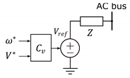 | 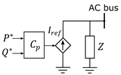 | 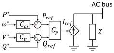 |
| Control inputs are voltage and frequency to assure grid stability | References of and power are given; PLL is needed for synchronization | Participation in the regulation of frequency and voltage , by and control |
| Resource | Dispatched | Resource | Load |
|---|---|---|---|
| MMC-HVDC-1 | 300 WM | Load 1 | 400 MW |
| MMC-HVDC-2 | 300 MW | Load 2 | 400 MW |
| SG 1 | 350 MW | Load 3 | 400 MW |
| SG 2 | 250 MW | Load 4 | 450 MW |
Publisher’s Note: MDPI stays neutral with regard to jurisdictional claims in published maps and institutional affiliations. |
© 2021 by the authors. Licensee MDPI, Basel, Switzerland. This article is an open access article distributed under the terms and conditions of the Creative Commons Attribution (CC BY) license (https://creativecommons.org/licenses/by/4.0/).
Share and Cite
Lourenço, L.F.N.; Perez, F.; Iovine, A.; Damm, G.; Monaro, R.M.; Salles, M.B.C. Stability Analysis of Grid-Forming MMC-HVDC Transmission Connected to Legacy Power Systems. Energies 2021, 14, 8017. https://doi.org/10.3390/en14238017
Lourenço LFN, Perez F, Iovine A, Damm G, Monaro RM, Salles MBC. Stability Analysis of Grid-Forming MMC-HVDC Transmission Connected to Legacy Power Systems. Energies. 2021; 14(23):8017. https://doi.org/10.3390/en14238017
Chicago/Turabian StyleLourenço, Luís F. N., Filipe Perez, Alessio Iovine, Gilney Damm, Renato M. Monaro, and Maurício B. C. Salles. 2021. "Stability Analysis of Grid-Forming MMC-HVDC Transmission Connected to Legacy Power Systems" Energies 14, no. 23: 8017. https://doi.org/10.3390/en14238017
APA StyleLourenço, L. F. N., Perez, F., Iovine, A., Damm, G., Monaro, R. M., & Salles, M. B. C. (2021). Stability Analysis of Grid-Forming MMC-HVDC Transmission Connected to Legacy Power Systems. Energies, 14(23), 8017. https://doi.org/10.3390/en14238017