Maximum Electrical Power Extraction from Sources by Load Matching

Abstract

This paper describes the matching of various loads to sources (including nonlinear ones). The purpose of matching is to extract the maximum available power from the source. This has particular importance for renewable sources and energy-harvesting devices, in which unused energy is just wasted. The main innovations in this paper include (and followed by examples) simplified calculation of the matching parameter for a controllable load and matching by means of a family of power-conservative two-port networks, denoted POPI (Pin = Pout), such as transformers, gyrators, loss-free resistors (LFRs) and series LFRs (SLFRs). An additional innovation described in this paper is a new, simplified model of an HF power amplifier based on the series LFR concept. This model predicts that the efficiency of the HF power amplifier operated under the matched-mode condition can significantly exceed the 50% efficiency limit that is predicted by the conventional model. As HF power amplifiers drive antennas in transmission and some wireless power transfer (which uses radiative techniques) systems, it is clear that the operation of such systems in the matched-mode condition is not restricted to a 50% efficiency limit.

1. Introduction

In electrical engineering, the maximum power transfer theorem states that, to obtain maximum external power from a source with a finite internal resistance, the resistance of the load must equal the resistance of the source, as viewed from its output terminals. Moritz von Jacobi published the maximum power (transfer) theorem around 1840; it is also referred to as “Jacobi’s law”.

The theorem results in maximum power transfer across the circuit but not maximum efficiency. If the resistance of the load is increased beyond the resistance of the source, then efficiency is higher because a higher percentage of the source power is transferred to the load, but the magnitude of the load power is lower because the total circuit resistance increases.

Extraction of the maximum available power is desirable in many systems involving sources and loads. This is attained by selecting a suitable load or, when possible, by controlling its parameters so that the source outputs its maximum available power. The operation of such systems is referred to as matched-mode operation. Operation in matched mode indicates that the source functions at the maximum power point (denoted MPP). The characteristic of the source determines the MPP voltage and current. In a family of systems that capture ambient energy and convert it into electrical energy, such as photovoltaic systems, wind generators and energy-harvesting devices, operation at MPP also implies maximum conversion efficiency of the ambient energy. This is because, in most of these cases, energy (solar irradiation, wind, etc.) cannot be stored in its original form, so the part that is not converted (to the electrical energy) is lost.

Systems that operate at MPP, such as those consisting of a voltage source and internal series resistance (storage battery, for example), result in high losses. It is evident that in such systems, operating at lower power than the maximum available is practical, preserving it for short instances in which high peak power is needed.

In this study, various source–load systems in matched-mode conditions were analyzed. These include linear and nonlinear systems, direct source–load connections and coupling by means of a power-conservative two-port network, denoted POPI (Pin = Pout), such as transformers, gyrators and loss-free resistors (LFRs). Various realizations of POPI networks (by means of switched-mode converters) are reported in [1,2,3,4,5,6,7]. Since power electronic circuits can be operated at high efficiency (up to 98%), using a family of POPI networks to model circuits is very convenient.

Some application examples of maximum power transfer by means of controlled POPI networks include photovoltaic systems, battery chargers and maximum energy extraction (from a decaying source) systems.

It should be noted that our paper is focused on cases in which the power needs of the load meet the maximum power ability of the source.

In all cases of curtailable loads, and in most cases of non-curtailable loads, the time-varying power demanded by the load differs from the maximum (time-varying) power that the source delivers; in order to bridge this difference, a storage element can be applied [8]. In that case, a controlled coupling network (realized by a converter, inverter or combination of both) is used in order to process the power flow between the source, load and storage so that the source operates at its maximum power point and fulfills the load requirements.

The combination of storage, load and a coupling network forms a new load (as viewed from the source) that can extract the maximum available power from the source. A typical example of an arrangement that includes a curtailable load is a standalone PV system [9,10]. In this system, the load power demand may vary or even be zero (load disconnection), whereas, during the entire operation period, the PV array can deliver the maximum available power to the load/storage system.

An example of a system that includes a non-curtailable load is a PV grid-connected system [11]. In that case, the grid is viewed from the PV array as a “black box” consisting of a voltage source, storage and load elements, and it is capable of absorbing all of the power that the source can deliver. In addition, in this case, matching is achieved by means of a coupling network consisting of a converter/inverter combination.

The conventional model of an RF power amplifier predicts that its operation in the matched-mode condition implies a 50% efficiency limit. However, some transmitters (with an RF power amplifier at the output stage) are known to operate at significantly higher efficiency (in the matched-mode condition) than is predicted by that model.

In order to resolve this contradiction, we propose a modified model that is based on the loss-free resistor concept. This model includes all of the properties of the classical model except the efficiency limit. The model was validated by simulations carried out over a practical transmission circuit.

2. Matching of Sources by Controllable Loads

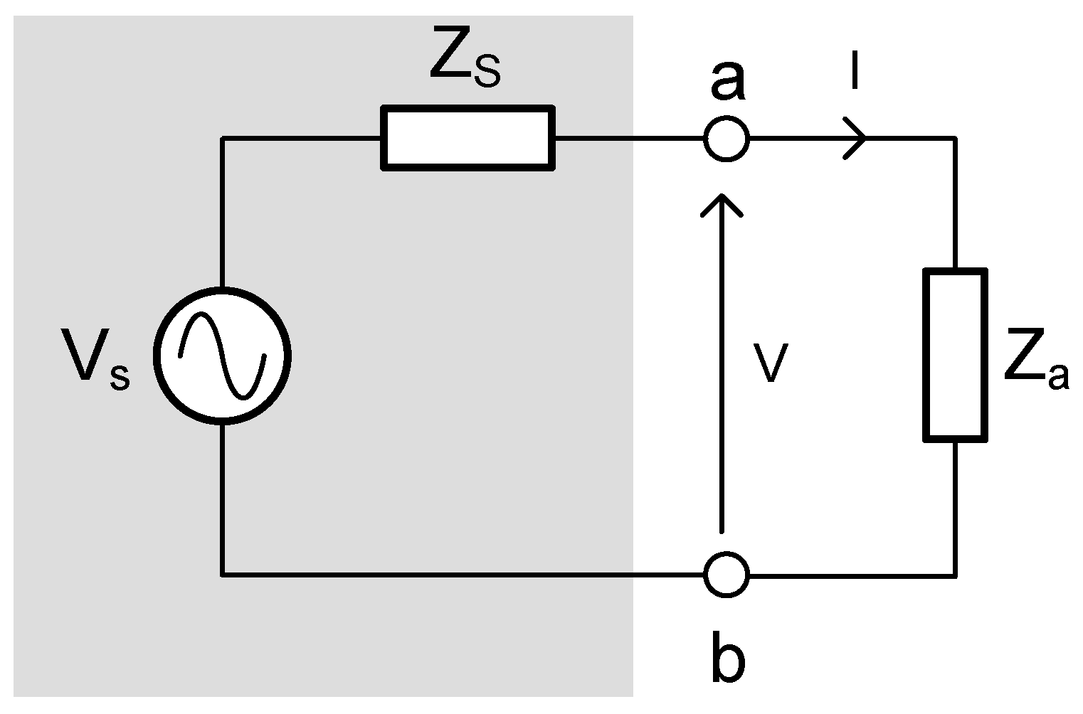
A conventional model of a large family of sources, such as batteries, generators, electromechanical devices, piezoelectric transformers and high-frequency and microwave transmission systems, consists of a voltage source and series resistance (or series impedance in the case of sine wave excitation). A voltage source with internal series resistance loaded with a resistive load is shown in Figure 1.

This model predicts that by loading the source with controlled resistance $R_L$, the maximum power can be extracted from the source by applying the conventional calculation method, i.e., $\frac{\partial P}{\partial R_L}=0$, resulting in $R_L=R_L^{*}=r_S$, where $R_L^{*}$ denotes the value of $R_L^{*}$ that extracts the maximum power from the source.

$$\begin{array}{l}{P}_{S\max }=\frac{1}{4}\frac{E^2}{r_S}\\ V_M=V_{a-b}=\frac{E}{2}\\ I_M=I_{a-b}=\frac{I_{SC}}{2}\\ I_{SC}\equiv \frac{E}{r_S}\end{array}\}$$

(1)

where $P_{S\max }$ denotes the maximum source power, and $V_M$ and $I_M$ are the voltage and current at the maximum power point, respectively.

It should be noted that the load should not be a resistive element only; for example, for a storage battery modeled with an ideal voltage source $u=u_b$, we have the following:

$$\begin{array}{l}i=i_{a-b}=\frac{V_S-u}{r_P}\\ P_{a-b}=i\cdot u=\left(\frac{V_S-u}{r_P}\right)u\\ \frac{\partial P_{a-b}}{\partial u}=\frac{V_S-2u}{r_S}\\ \frac{\partial P_{a-b}}{\partial u}=0\Rightarrow V_M=U^{*}=\frac{V_S}{2}\end{array}$$

(2)

Inserting $V_M$ into the current equation results in the following:

$$\begin{array}{l}{I}_M=\frac{V_S}{2r_S}=\frac{I_{SC}}{2}\\ P_{a-b\max }=V_M{I}_M=\frac{V_S^2}{4r_S}\end{array}$$

(3)

3. Efficiency of a Source with Internal Resistance in Matched-Mode Operation

The efficiency, $\eta$, is given by the following:

$$\eta =\frac{P_{out}}{P_{in}}=\frac{v_{a-b}\cdot i_{a-b}}{P_{in}}$$

(4)

$P_{in}$ is the power delivered by $V_S$, including the load power and the internal losses on $r_S$:

$$\begin{array}{l}{P}_{in}=V_{S}i=V_S{i}_{a-b}\\ P_o=P_{load}=v_{a-b}\cdot i_{a-b}\end{array}$$

(5)

In matched-mode operation:

$$\begin{array}{l}{i}_b=I_M=\frac{I_{SC}}{2}\\ V_{a-b}=V_M=\frac{V_S}{2}\\ \eta =\frac{V_M{I}_M}{V_S{I}_M}=\frac{V_M}{V_S}=0.5=50\%\end{array}$$

(6)

This result is general and independent of the kind of load that enables the source to operate at the maximum output power.

4. AC Source with Internal Impedance

The phasor description of an AC source ${\overline{V}}_S$ with internal impedance $Z_S$ loaded by $Z_a$ is shown in Figure 2.

The source and load impedances are given by the following:

$$\begin{array}{l}{Z}_S=r_s+j{x}_S\\ Z_a=r_a+j{x}_a\end{array}\}$$

(7)

It is well known that maximum power transfer, $P_{\max }$, is achieved when the load $Z_a=Z_S^{*}$:

$$\begin{array}{l}{X}_a=-X_S\\ r_a=r_S\end{array}$$

(8)

In this case, $P_{S\max }$ and the power transfer efficiency, $\eta$, are given by the following:

$$P_{S\max }=\frac{{\overline{V}}_S^2}{4r_S}$$

(9)

$$\eta =50\%$$

(10)

5. Matching General Sources to Controllable Loads

Let us analyze the case in which a source consisting of voltage source $E$ with internal resistance $r_P$ is loaded with a nonlinear load (which approximately describes the characteristic of an LED string), given by the following:

$$i=a{e}^{\frac{v}{v_0}}$$

(11)

where a is controllable. Attempting to find $a^{*}$ (the value of a that extracts the maximum source power $P$) using the classical method (i.e., $\frac{\partial P}{\partial a}=0\Rightarrow a_{*}=\cdots$) is quite a difficult task. The difficulty increases if the source has nonlinear characteristics (in many cases, there is no closed-form solution).

A much easier calculation is based on the insight that the maximum power is a property of the source (of any source), and the suitable load just enables the extraction of that power, so we can substitute the maximum power point coordinates ($V_M, I_M$) into the load characteristic in order to obtain the solution with a simpler method. In our case, for example, we have the following:

$$\begin{array}{l}i=I_M\\ v=V_M\end{array}\}$$

(12)

$$a=a^{*}=I_M{e}^{-\frac{V_M}{V_0}}$$

(13)

In our source, $V_M=\frac{E}{2},I_M=\frac{I_{SC}}{2}\left(I_{SC}=\frac{E}{r_P}\right)$; therefore, we have the following:

$$a^{*}=\frac{I_{SC}}{2}{e}^{-\frac{E}{2V_o}}$$

(14)

If the source and the load both have nonlinear characteristics, it is recommended to calculate the voltage and current at the MPP (maximum power point), denoted $V_M$ and $I_M$, and to then insert the values into the load $i-v$ curve in order to determine the matching conditions.

An example is a system in which the source characteristics are given by the following:

$$V_S=E-\beta \cdot i_S^2$$

(15)

This equation is a reasonable approximation of a typical fuel cell with a particular focus on its MPP domain.

The load $i-v$ curve is given by the following:

$$i=a\cdot e^{\frac{u}{V_o}}$$

(16)

The source MPP parameters are calculated as follows:

$$\begin{array}{l}{P}_S=v_S{i}_S=\left(E-\beta \cdot i_S^2\right)i_S\\ \frac{\partial P}{\partial i_S}=0\Rightarrow E-3\beta \cdot i_S^2=0\\ i_S^{*}\equiv I_M=\sqrt{\frac{E}{3\beta }}\\ v_S^{*}\equiv V_M=\frac{2}{3}E\\ P_{S\max }\equiv P_M=\frac{2}{3}E\sqrt{\frac{E}{3\beta }}\end{array}$$

(17)

Inserting $V_M$, $I_M$ into the load characteristic implies that the value of $a$ that extracts the maximum power, denoted $a^{*}$ is given by:

$$a^{*}=\sqrt{\frac{E}{3\beta }}{e}^{-\frac{2E}{3v_o}}$$

(18)

6. Voltage Source Type with a Fuse

In many practical systems, the load is operated at a much lower current than the short-circuit current; the current is limited by a fuse that is destroyed at currents higher than $I_F$ (the same can be achieved by an overload relay or by the collapse of some component in the circuit see Figure 3).

As the maximum current that the source can deliver is limited by $I_F$, this value determines the maximum power point current and voltage as follows:

$$\begin{array}{l}{I}_M=I_F\\ V_M=\left(V_S-I_F{r}_S\right)\\ P_{S\max }=I_F\left(V_S-I_F{r}_S\right)\end{array}$$

(19)

As $I_F$ is much lower than the short circuit, $I_{SC}$, this value of power is much lower than that in a case involving only the voltage source and internal resistance (given in Equation (1)) In this case, the efficiency is given by the following:

$$\eta =\frac{I_F\left(V_S-r_S{I}_F\right)}{V_S{I}_F}=1-\frac{I_F{r}_S}{V_S}$$

(20)

If $\frac{I_F{r}_S}{E}\ll 1$, then $P_{a-b\max }\to I_F{V}_S$, and the power transfer efficiency is $\eta \to 1$.

If the load is controllable, the load parameters that result in maximum power transfer can be determined by inserting the maximum power point coordinates ($I_M$, $V_M$), as described previously.

It should be noted that because the fuse (or current limiter) is installed for safety purposes, most practical systems are operated at power levels that are significantly lower than that determined by $P_{S\max }$.

7. Matching by Means of Controlled Two-Port Networks

In most cases, the load is not tunable, so matching can be achieved by applying a power-conservative two-port element whose parameters can be controlled. There is a family of power conservative two-port network elements in which the output power equals the input power:

$$P_o\left(t\right)=v_o\left(t\right)i_o\left(t\right)=P_i\left(t\right)=v_{i\left(t\right)}{i}_{i\left(t\right)}\forall t$$

(21)

A network element that satisfies Equation (19) Is denoted POPI $\left(P_o\left(t\right)=P_i\left(t\right)\right)$, see Figure 4.

Transformers, gyrators and loss-free resistors (LFRs) are among the elements in the POPI family (Figure 5).

The governing relations between the input and the output electronic parameters of the different models are summarized next.

For the LFR:

$$\begin{array}{l}{i}_1=\raisebox{1ex}{$v_1$}\!\left/ \!\raisebox{-1ex}{$R_E$}\right.\left(t\right)\\ p_2=p_1\end{array}\}$$

(22)

For the TVT:

$$\left[\begin{array}{c}{v}_1\\ i_1\end{array}\right]=\left[\begin{array}{cc}k\left(t\right)& 0\\ 0& k{\left(t\right)}^{-1}\end{array}\right]\left[\begin{array}{c}{v}_2\\ i_2\end{array}\right]$$

(23)

For the gyrator, the governing relation is as follows:

$$\left[\begin{array}{c}{i}_1\\ v_1\end{array}\right]=\left[\begin{array}{cc}0& g\left(t\right)\\ g{\left(t\right)}^{-1}& 0\end{array}\right]\left[\begin{array}{c}{i}_2\\ v_2\end{array}\right]$$

(24)

where, in the above models, the controlled parameters are $R_E\left(t\right)$, $k\left(t\right)$ and $g\left(t\right)$, respectively. The controlled parameter is chosen in a way that accommodates the constraints of the load and source.

It should be noted that in addition to the above-mentioned networks, additional two-port networks share the POPI property and other types of characteristics.

POPI networks can be realized by a variety of switched-mode converters operated at high switching frequency. For example, pulse-width modulation (PWM) converters can realize the transformer; some topologies of a series resonant converter and discontinuous conduction mode (DCM) exhibit gyrator characteristics [1,2,3], and a PWM DCM buck-boost converter can operate as an LFR [1].

As an example, two methods of LFR realization are described next. The first method is based on the continuous control of a PWM converter operated in CCM in such a way that the input current and voltage parameters obey Ohm’s law, resulting in the creation of an emulated resistance $R_E$. Then, the power absorbed by $R_E$ is transferred to the output terminals, forming the LFR [4].

The “natural” (i.e., non-controlled) realization of the LFR is based on the buck-boost converter topology operated in DCM (Figure 6a,b). In this converter, the voltage to average current ratio calculated at the input terminal is as follows:

$$\frac{V_{in}}{I_{in}}=R_E=\frac{2L}{D_1{}^2\cdot T_S}$$

(25)

where $D_1$ is the duty cycle, $T_S$ is the switching time interval and $L$ is the inductance of the inductor. As all variables in (23) are constant, this imparts resistive characteristics to the input terminals, i.e., emulates a resistance, denoted as $R_E$ (Figure 6a).

The power absorbed by the input terminals is transferred to the output (as a result of the ideal converter characteristics).

The realization is completed by averaging the pulsating current at the input by means of a low-pass filter, as shown in Figure 5c.

It should be noted that other realizations of POPI networks exist and that in addition to the transformer, gyrator and LFR, there are additional elements in the large family of POPI networks that are characterized by different properties. Applications of such networks in power processing systems are described in [6,7,8,12,13,14,15,16].

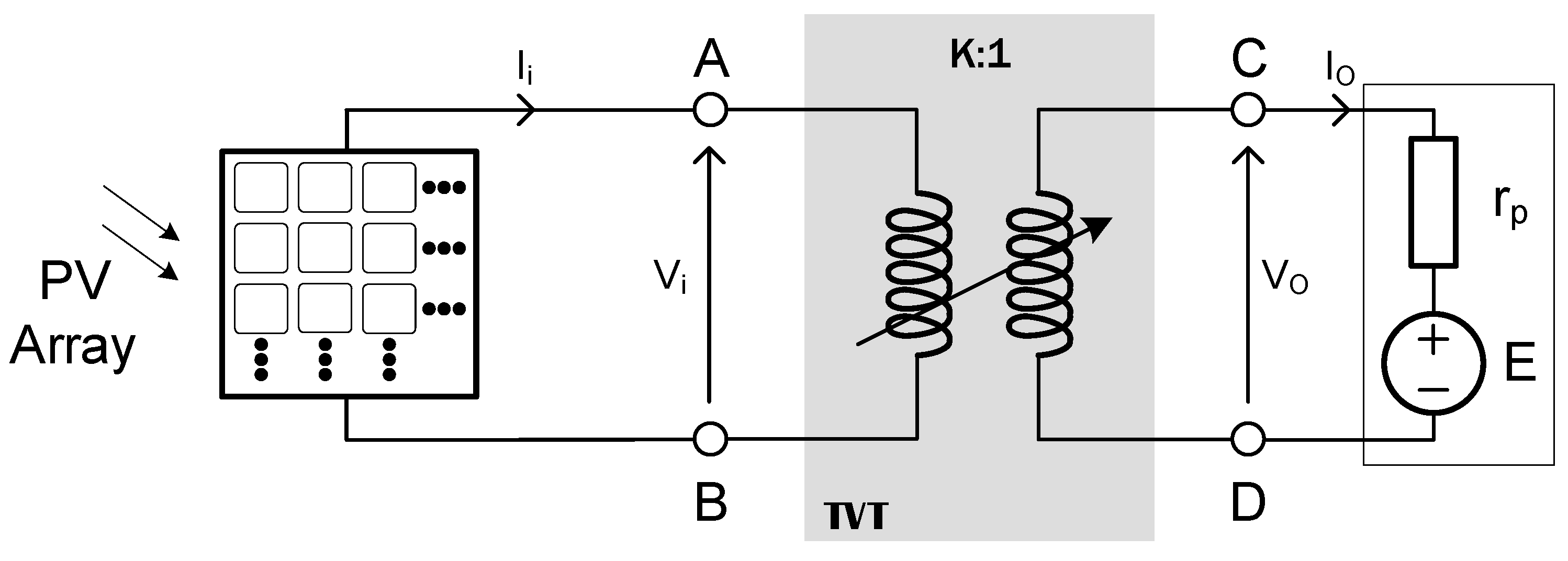
8. Matched-Mode Operation of a Photovoltaic System

The intersection of PV array and typical load characteristics is shown in Figure 7.

It should be noted that in practical photovoltaic systems, most loads can be described as comprising a voltage source E in series with a resistive element r_p. In most cases, the voltage source is the efficient part of the load, and the resistor is the part with losses. This description applies to a standalone PV system with a storage battery PV system, connected to the utility and PV array, or a PV array that powers an electrical motor (for pumping purposes).

A load connected directly to a PV array will very rarely extract the maximum power from the array (Figure 7).

In order to extract the maximum available power [17], we can match the load to the PV array by means of a POPI two-port element, for example, by means of a transformer, because the I–V curve of the PV array varies with the insulation, and the load parameters may vary as well, so dynamic matching is necessary. Dynamic matching can be achieved by controlling the transfer ratio of the transformer so that the transfer load intersects the maximum power point $V_M, I_M$ of the array (Figure 8). The transformer equations are as follows:

$$\left[\begin{array}{c}{v}_i\\ i_i\end{array}\right]=\left[\begin{array}{cc}k\left(t\right)& 0\\ 0& k^{-1}\left(t\right)\end{array}\right]\left[\begin{array}{c}{v}_o\\ i_o\end{array}\right]$$

(26)

By transferring the load to the input terminals of the transformer, the equivalent circuit is given by the following (Figure 9):

The circuit equation is given by the following:

$$v_i=i_i{r_P}^{\prime }+E^{\prime }$$

(27)

The transferred resistance $r^{\prime }$ and voltage $E^{\prime }$ are given by the following:

$$\begin{array}{l}{r}^{\prime }=r_P\cdot k^2\left(t\right)\\ E^{\prime }=E\cdot k\left(t\right)\end{array}$$

(28)

The circuit becomes the following:

$$v_i=i_i{k}^2{r}_P+kE$$

(29)

As we are interested in operating the circuit at the maximum power point $V_M, I_M$, replacing the general $k$ with that which enables operation at this power point, denoted $k^{*}\left(t\right)$, results in the following:

$$I_M{r}_p{k}^2\left(t\right)+k^{*}\left(t\right)E=V_M$$

(30)

The solution is as follows:

$$\left\{\begin{array}{l}{k}^{*}\left(t\right)=\frac{1}{2}\left[\frac{V_M}{E}+\sqrt{{\left(\frac{V_M}{E}\right)}^2+4\frac{r_P}{R_M}}\right]\\ R_M=\frac{V_M}{I_M}\end{array}\right\}$$

(31)

9. Matching a PV Array to a Load by Means of LFR

The matching of a PV array to a load can be achieved by coupling the array to the load by means of a loss-free resistor (LFR) [18]. As described previously, the LFR is a power-conservative two-port network (POPI) whose input terminals are buffered from the output. The input terminal has a resistive characteristic, which is modeled by a resistive element $R_E$, and the output has a power source with features in the $i-v$ curve. The power that is absorbed by $r_E$ is transferred to the output terminals and creates the power source characteristic (see Figure 10).

Matching is achieved by controlling $R_E$ such that its value is given by the following:

$$\begin{array}{l}{R}_E=R_E^{*}=R_M\\ R_M=\frac{V_M}{I_M}\end{array}$$

(32)

where $V_M$ and $I_M$ are the voltage and current of the PV array at MPP, respectively. Equation (30) implies the maximum power transfer to the load.

When matching with a loss-free resistor (Figure 11), we control the value of the emulated resistance, $r_E$, of the loss-free resistor such that $r_E=r_E^{*}$, which implies the maximum power transfer.

$$R_E^{*}=R_M=\frac{V_M}{I_M}$$

(33)

An advantage of matching is the fact that the output is buffered from the input terminals in the two-port network, so load variations do not affect the matching.

10. Finding the Matching Parameter of the POPI by Load Current Measurement

In the conventional control of a photovoltaic system, we determine the instantaneous maximum power of the array by measuring the output voltage and current of the array, as well as their multiplications, and varying the parameters of the matching network to determine the maximum value. For a load consisting of a resistance in series with a voltage source, the voltage and current are increasing functions of the input power [19]:

$$P=p_{\max }\to \begin{array}{c}{v}_{load}=v_{\max }\\ i_{load}=i_{\max }\end{array}\}$$

(34)

Therefore, coupling a source with nonlinear characteristics to any two ports results in a power-conservative two-port network whose internal parameter x can be controlled, as illustrated in Figure 12.

We do not need to multiply the two measurements $V_S,I_S$ in order to find the power and then apply the load to determine its maximum value: it is sufficient to vary the parameter $x$.

By measuring the load current, when $I$ reaches its peak, we know that the source delivers the maximum available power. The parameter $x$ that produces this maximum power is denoted by $X^{*}$. This type of control requires fewer measurements (output current instead of input voltage and current) and multiplication, enabling the construction of simpler PV systems. It should be noted that the practical process described above is also suitable for a matching network with some losses with constant efficiency.

11. Maximum Energy Extraction from a Decaying Source

An example of a situation requiring dynamic matching is that of storing the maximum available energy in loss-free storage. Let $V_S$ be a pulse source that decays exponentially with time, with internal resistance Rs coupled to a loss-free storage system by means of a controlled power-conservative network (POPI), as shown in Figure 13.

For $V_S\left(t\right)$, given by Equation (33), and an internal resistor, $r_S$, the maximum power is given by Equation (34).

$$v_S\left(t\right)=E\cdot e^{-\frac{t}{\tau }}$$

(35)

$$p_{\max }\left(t\right)=\frac{1}{4r_S}{V}_S^2\left(t\right)=\frac{E^2}{4r_S}{e}^{-\frac{2t}{\tau }}$$

(36)

In order to transfer the maximum available energy to the storage element, we must extract the maximum available power from the source during the entire process:

$$w_{\max }={\displaystyle \underset{t=0}{\overset{\infty }{\int }}{p}_S\left(t\right)dt=\frac{E^2}{8r_S}\tau }$$

(37)

For capacitive storage $c$ whose initial voltage is ${v_c|}_{t=}=v_{c0}\to 0$ (Figure 14), we have the following:

$$w_c\left(t\right)={\displaystyle \underset{t=0}{\overset{t}{\int }}{p}_{S\max }\left(t\right)dt}=\frac{E^2}{8r_S}\tau \left(1-e^{-\frac{2t}{\tau }}\right)$$

(38)

Therefore, the voltage at terminals $C-D$ is given by the following:

$$v_c\left(t\right)=\sqrt{\frac{2}{C}\frac{E^2}{8r_S}\tau \left(1-e^{-\frac{2t}{\tau }}\right)}=\frac{E}{2}\sqrt{\frac{\tau }{r_{S}C}\left(1-e^{-\frac{2t}{\tau }}\right)}$$

(39)

The process is controlled by a time-varying transformer whose transfer ratio is $k\left(t\right)$.

$k\left(t\right)$ is given by the following:

$$k\left(t\right)=\frac{\raisebox{1ex}{$E$}\!\left/ \!\raisebox{-1ex}{$2$}\right.}{v_2\left(t\right)}=\frac{e^{-\frac{t}{\tau }}}{\sqrt{\frac{\tau }{r_{S}C}\left(1-e^{-\frac{2t}{\tau }}\right)}}$$

(40)

When matching with a loss-free resistor, the maximum power energy transfer is achieved. $R_E$ has a constant value that equals $r_S$:

$$R_e=R_S\forall t$$

(41)

In a case in which the storage device is a battery with open-circuit voltage, $E$, and leakage modeled by parallel resistance, $r_b$ (Figure 15), it is of interest to determine the time at which the stored energy reaches its maximum. This occurs when the maximum power of the source equals the leakage power.

The time $t_1$ in which the maximum source power equals the leakage losses is given by the following:

$$\begin{array}{l}{P}_{S\max }-P_{r_{b}losses}\Rightarrow \frac{E^2}{r_b}\to \frac{E^2}{4r_S}{e}^{-\frac{2t}{\tau }}-\frac{E^2}{r_b}=0\\ t_1=\frac{\tau }{2}\ln \left(\frac{r_b}{4r_S}\right)\end{array}$$

(42)

After $t=t_1$, the power loss is greater than the power supplied by the source, so at $t=t_1$, the energy that accumulates in the battery reaches its maximum value:

$$\begin{array}{l}{w}_{stored}={\displaystyle \underset{t=0}{\overset{t-t_1}{\int }}{P}_{S\max }\left(t\right)dt-\frac{E^2}{r_b}{t}_1=}\\ =\frac{E^2}{r_b}\left[\frac{\tau }{8}\left(1-e^{-\frac{2t_1}{\tau }}\right)-\frac{r_S}{r_b}{t}_1\right]=\\ =\frac{E^2}{r_b}\left[\frac{\tau }{8}\left(1-e^{-\frac{2t_1}{\tau }}\right)-\frac{r_S}{r_b}\frac{\tau }{2}\ln \left(\frac{r_b}{4r_S}\right)\right]=\\ =\frac{E^2}{r_b}\frac{\tau }{2}\left[\frac{1}{4}\left(1-e^{-\frac{2t_1}{\tau }}\right)-\frac{r_S}{r_b}\frac{\tau }{2}\ln \left(\frac{r_b}{4r_S}\right)\right]\end{array}$$

(43)

12. Battery Charger

A battery charger can be constructed by means of a circuit based on the POPI concept. In many cases, the charger is supplied by a DC source $V_S$ with a fuse that is destroyed at currents higher than $I_F$. The typical battery can be modeled by a voltage source $E_b$ with series resistance $r$; in most cases, the voltage drop in $r$ can be neglected (compared to $E_b$).

Previous studies have shown that such source–load coupling by means of a transformer is associated with sensitivity problems [4] (of source and load currents to voltage variations), so applying a circuit based on a gyrator or LFR concept is preferable.

The coupling circuit controls the source current such that $i_S\le I_F$. In an extreme case in which $i_S$ equals $I_F$, the highest power transfer is achieved, resulting in the highest charging rate. Figure 16 illustrates this process for a gyrator-based charger.

The source current is given by the following:

$$i_{S|i_S\le I_F}=Y_{eq}{V}_S+I_{eq}=g^{2}r+g{E}_b$$

(44)

In most cases, $r$ can be neglected, so (42) can be reduced to the following:

$$i_{S|i_S\le I_F}\simeq g{E}_b$$

(45)

The highest power transfer is achieved when $i_S=I_F$, resulting in the fastest battery charging, so $g^{*}$ that produces this current is given by the following:

$$\begin{array}{l}{g}^{*}=\frac{I_F}{E_b}\\ g=g^{*}\to P_S=P_{S\max }=I_F{V}_S\end{array}$$

(46)

Then, the battery charging current is as follows:

$$i_{b\max }\simeq \raisebox{1ex}{$P_{S\max }$}\!\left/ \!\raisebox{-1ex}{$E_b$}\right.\simeq I_F\left(\frac{V_S}{V_b}\right)$$

(47)

Controlling the value of $g$ such that (45) is satisfied results in the fastest possible charging rate of the battery.

13. Marched-Mode Operation of RF Power Amplifier

Basic applications of an RF power amplifier include driving to another high-power source, driving a transmitting antenna and exciting microwave cavity resonators. Among these applications, driving transmitter antennas are the most well known.

A simplified model of a transmission system consisting of a transmitter and antenna that is fed directly by the RF power amplifier output (the output stage of the transmitter) is shown in Figure 17a. In this figure, the RF power amplifier is modeled by a “black box”, which includes the arrangement of various elements (amplifying devices, resonant tanks, LC filters, segments of transmission lines, etc.). This “black box” extracts DC power from a DC source, $E$, and converts it into high-frequency power that is transferred to the antenna.

The simplest conventional electrical equivalent circuit (Figure 17b) of this model consists of a high-frequency voltage source ${\overline{V}}_S$, with internal impedance ${\overline{Z}}_S$ (the electrical equivalent of the “black box” output as viewed from the antenna) and the antenna impedance $Z_a$ [20].

As in the case of the previously analyzed AC source, maximum power is extracted when ${\overline{Z}}_S^{*}={\overline{Z}}_a$ (Figure 18):

$$\begin{array}{l}{r}_S=r_a\\ x_S=-x_a\end{array}$$

(48)

In this case, the efficiency, as calculated previously, is as follows:

$$\eta =\frac{P_a}{P_S}=\frac{i^2{r}_a}{\begin{array}{l}{i}^2\left(r_a+r_S\right)\\ r_a=r_S\Rightarrow \eta =50\%\end{array}}$$

(49)

The total conversion efficiency of the transmission system from DC into a high frequency is given by the following:

$${\eta }_{tot}=\frac{P_{RF}}{P_{dc}}$$

(50)

where $P_{RF}$ is the high-frequency power delivered to the load (antenna) by the “black box” (Figure 17a), and $P_{dc}$ is the DC power delivered by the voltage source E to the “black box” $a-b$ terminals.

As shown previously (in the case of the AC source with internal impedance loaded by AC impedance), the theoretical model (Figure 5) predicts an efficiency of 50% in matched-mode operation. On the other hand, although the measured overall system efficiency is below this limit in many cases, it often exceeds 50% in other cases. Clearly, efficiencies lower than this value (even in matched mode) are expected, as practical systems encounter losses that are not predicted by the theoretical model. However, situations in which practical systems exhibit efficiencies greater than 50% are surprising; these cannot be explained by the traditional model.

This contradiction can be resolved by replacing the resistive part of the source impedance with a series loss-free resistor (SLFR) (Figure 19). The basic LFR (described in the previous section) is a two-port network with an element, $R_E$, at its input terminals and an element defined as a power source at its output, whose power equals that absorbed by the resistance part $R_E$ (Figure 19a).

The SLFR concept, introduced by Ivo Barbi [21], is a topological transformation of the basic LFR model, in which the emulated resistance $R_E$ is connected between the input and the output and the power source, $P$, in parallel to the input (Figure 19b).

The losses that occur during the operation of a practical system can be modeled by slightly modifying the SLFR, denoted semi-SLFR. In this case, we assume that only part of the power that is absorbed by $R_E$ is transferred to the input SLFR terminals, i.e., $P=\alpha P_{RE}\left(0\le \alpha \le 1\right)$ (see Figure 19c).

A practical system experiences some losses, so the SLFR model can be modified to one with some losses by multiplying the power transferred from the other $R_E$ to the power source by an efficiency transfer factor $\alpha$; i.e., the power that is transferred from $R_E$ and creates the power source (of the SLFR), $P$, whose power is returned to $V_S$, is as follows:

$$P=\alpha P_{RE}\left(0\le \alpha \le 1\right)$$

(51)

Replacing the resistive part of ${\overline{Z}}_S$ (Figure 17) with a semi-SFLR results in the modified transmission system model shown in Figure 20. The power transfer efficiency of that circuit is as follows:

$${\eta }_{\overline{V}s}\equiv \raisebox{1ex}{$P_S$}\!\left/ \!\raisebox{-1ex}{$P_a$}\right.$$

(52)

where $P_S$ is the total (high-frequency) power supplied by ${\overline{V}}_S$, and $P_a$ is the power absorbed by the load (antenna).

In the matched-mode condition, ${\eta }_{\overline{V}S}$ is given by the following:

$${\eta }_{\overline{V}S}=\raisebox{1ex}{$1$}\!\left/ \!\raisebox{-1ex}{$\left(2-\alpha \right)$}\right.$$

(53)

As $\alpha$ may vary in the range $0\le \alpha \le 1$, the power transfer efficiency may vary between 50 and 100% in the matched-mode condition.

As this model predicts that the efficiency of the internal model (consisting of ${\overline{V}}_S$, ${\overline{Z}}_S$ and ${\overline{Z}}_a$) can exceed a value of 50%, there is no contradiction between that result and the total measured efficiency (it is impossible for the total efficiency to be higher than that of the internal model). As RF power amplifiers find applications in a variety of systems (communication, microwave, wireless power transfer), further understanding their efficiency limit is important.

We do not claim that practical systems actually contain an LFR; we only claim that this model describes the behavior of an efficient type of such systems operating in matched-mode conditions. The fact that there are some elements that have resistive characteristics that do not produce losses (in principle only), such as segments of transmission lines and resonant tanks [22,23,24] in the RF power amplifier, motivated us to propose the model described above.

14. Simulation Results of Transmission System

A practical transmission system consisting of an HF power amplifier and antenna was designed and simulated (using ADS simulation software) in order to evaluate the power transfer efficiency (of that system) in the matched-mode condition (Figure 21).

The system was designed to be operated at a frequency of 250 MHz and powered by a 28 V DC voltage source.

The transmitter was designed to have an output impedance that is purely resistive (50 Ω), and the load is a variable pure resistive element that represents the antenna.

It was found that the maximum power was transferred to the load when the load resistance was equal to the output impedance of the transmitter (50 Ω), and the reflection coefficient tended to zero (Figure 22). Voltage and current waveforms (in the matched condition) at the transistor drain and voltage on the load (antenna) are shown in Figure 23.

At that point, the output RF power was 10.7 W, and the DC supply current and voltage were 0.51 A and 28 V, respectively, so the total efficiency was approximately 75%.

Based on these results, it is clear that in matched-mode operation, the transfer efficiency can be significantly higher than 50%, so our proposed model based on the loss-free resistor concept is suitable for a simplified description of real transmission system behavior.

15. Conclusions

This paper describes the operation of source–load systems in which the load is adjusted to the source such that the maximum available source power is extracted, which (mode of operation) is called matched-mode operation. A matched-mode operation is achieved by controlling the load parameter (if possible) or by using the proposed power-conservative two-port network, such as a gyrator or loss-free resistor (LFR). The “classical” calculation of the controllable load parameter X (or of the matching network parameter) is based on $\frac{\partial P_o}{\partial x}=0\Rightarrow X=X^{*}$, where $P_o$ is the load power and $X^{*}$ is the value of $X$ that results in $P_o=P_{o\max }$. It has been found that this calculation method may be very difficult to apply if the source, load or both are nonlinear. Therefore, we propose a simple method to derive the $X^{*}$ parameter. The calculation method is based on the observation that the maximum power point (MPP) coordinates of the source, that is, the MPP voltage $V_M$ and current $I_M$, are characteristics of the source only, so there is no need to go through the $\frac{\partial P_o}{\partial x}=0\Rightarrow X=X^{*}$ process, because we can simply substitute the coordinates of the voltage and current of the source at maximum power point coordinates $V_M$ and $I_M$ into the load $i-v$ curve in order to obtain the value of $X^{*}$.

As controllable loads are quite rare, matching by means of power-conservative two-port networks can be realized by means of a variety of switched-mode converters operated at a high switching frequency. As an example, the “natural” realization of a loss-free resistor (LFR) is presented.

Examples of matching by means of these networks include photovoltaic systems, transferring maximum available energy from a decaying source to storage, and fast battery chargers.

A simple modified model of the RF power amplifier loss-free resistor concept is proposed. The model predicts that, in the matched-mode operation, the 50% efficiency limit implied by the classical model can be significantly exceeded, so the total efficiency of a system that includes an RF power amplifier at its output stage (communication, microwave, and wireless power transformer), in which maximum power is extracted, can also exceed this limit.