Survey and Comparison of Optimization-Based Aggregation Methods for the Determination of the Flexibility Potentials at Vertical System Interconnections

Abstract

The aggregation of operational active and reactive power flexibilities as the feasible operation region (FOR) is a main component of a hierarchical multi-voltage-level grid control as well as the cooperation of transmission and distribution system operators at vertical system interconnections. This article presents a new optimization-based aggregation approach, based on a modified particle swarm optimization (PSO) and compares it to non-linear and linear programming. The approach is to combine the advantages of stochastic and optimization-based methods to achieve an appropriate aggregation of flexibilities while obtaining additional meta information during the iterative solution process. The general principles for sampling an FOR are introduced in a survey of aggregation methods from the literature and the adaptation of the classic optimal power flow problem. The investigations are based on simulations of the Cigré medium voltage test system and are divided into three parts. The improvement of the classic PSO algorithm regarding the determination of the FOR are presented. The most suitable of four sampling strategies from the literature is identified and selected for the comparison of the optimization methods. The analysis of the results reveals a better performance of the modified PSO in sampling the FOR compared to the other optimization methods.

1. Introduction

1.1. Motivation

The transition of the electrical power system leads to a massive integration of decentralized energy resources (DER), primarily in the distribution system level. Thereby, the conventional energy supply by thermal power plants at the transmission system level are substituted through decentralized, controllable and flexible converter-coupled system elements (e.g., DER) at the distribution system level. The vertical power flows become increasingly volatile depending on the load situation and availability of primary energy. Therefore, the transmission system operators (TSO) are confronted by new challenges to guarantee a safe and reliable system operation in the future, including new operational efforts due to the shift of ancillary service potentials to the distribution system level. Measures like grid expansions or the integration of new flexibilities at the transmission grid (e.g., synchronous condenser) are expensive. To avoid this, another option is the coordinated interaction of TSO and distribution system operators (DSO) [1]. This TSO/DSO cooperation is enabled by an advanced monitoring of the current grid states and the control of distributed flexibilities (e.g., reactive power supply of wind turbines, load management) through the continuous integration of information- and communication technology (ICT) [2]. The previous passive distribution system level with limited flexibilities within the operational management of the DSO transforms to an active distribution system level with a variety of control options. The utilization of the distributed flexibilities also leads to a change of the vertical active and reactive power flows. Therefore, flexibilities that are located at the distribution system can potentially be used for the operational management of the TSO [3].

In the recent years the ENTSO-E [4,5,6,7,8] and Cigré [9] are focused increasingly on the topic of TSO/DSO cooperation to provide a maximum of assured flexibility potentials from the distribution to the transmission system level. Thereby, the first step is to include the distributed flexibility potentials at the day-ahead or intraday operational planning of the TSO while avoiding a conflicting or counter-acting use of flexibilities. For this vertical supply of ancillary services, a suitable multi-voltage-level grid control concept needs to be developed, defining the interactions and communication between the TSO and DSO. Hierarchical grid control concepts are an opportunity besides currently not achievable central or fully-distributed grid control concepts (e.g., system operator responsibilities, regulatory frameworks, big data, privacy aspects, ICT integration). A taxonomy and overview of hierarchical, also known as vertical-distributed, TSO/DSO coordination schemes are provided in [10,11], respectively. Hierarchical grid control concepts consider the conventional separation of the operational management of the system operators [12]. TSO/DSO interactions are based on a feasible operation region (FOR) (see left side of Figure 1, also known as active and reactive power (PQ) flexibility area, equivalent PQ-capability, PQ-flexibility map), which represents the aggregated flexibility potentials for the adaptation of the vertical active and reactive power flows ($P_{\mathrm{vert}}$, $Q_{\mathrm{vert}}$) at the TSO/DSO interconnections [13]. The FOR is determined by the DSO under consideration of the current grid state to guarantee a compliance of technical constraints (e.g., voltage limits, thermal capacity of lines and transformers). Operational degrees of freedom are flexibility providing units (FPU, see right side of Figure 1) of the DSO (e.g., on-load tap changing (OLTC) transformer, compensation systems) as well as distributed flexibility potentials (e.g., controllable loads, DER). The FOR can be integrated in the operational management of the TSO as an additional reactive and active power flexibility while the compliance of a certain set-point ($P_{\mathrm{vert},\mathrm{sp}}$, $Q_{\mathrm{vert},\mathrm{sp}}$) and the coordination of the distributed flexibility supply are performed by the DSO [14]. Thereby, the complexity of multi-voltage-level grid control is reduced and the individual interests of the DSO and the stakeholder of the FPU can be considered, e.g., by a monetarization of the FOR area.

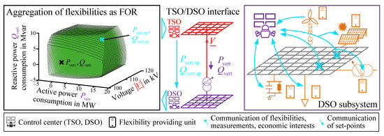
Figure 1. Aggregation of DSO flexibilities for the TSO by a FOR at the TSO/DSO interface.

Various methods for the determination of the FOR are introduced in literature. In addition, the application of the approach at the DSO/DSO interface in the context of a DSO/DSO cooperation and thus, an extension of the hierarchical multi-voltage-level grid control concept to the overall system are discussed.

1.2. Related Work

The approach of describing the flexibility potential at the TSO/DSO interface by a PQ-plane was first described in [15]. A Monte-Carlo simulation is performed based on a variety of random control scenarios by assigning set-values from an uniform distribution for each active and reactive power flexibility capable device [15]. The vertical active and reactive power flows at the TSO/DSO interface are determined by a power flow calculation for each scenario. The resulting point cloud at the PQ-plane specifies the FOR. Control scenarios, which lead to a violation of technical constraints are neglected to consider just feasible operating points. Individual cost factors for the active and reactive power supply of the FPU are considered and the resulting flexibility costs at the TSO/DSO interface determined. The quality of the resulting FOR decreases with an increase of the individual flexibilities, because of the central limit theorem of the probability theory [16]. A negative correlation between generation and load at the same bus is implemented to deal with this. The authors in [15] recommend the formulation of an optimization problem for a more detailed sampling of the FOR edges.

In [17], the stochastic approach of [15] is extended by describing the flexibility potential at the TSO/DSO interface by a polygon based on the contour of the FOR point cloud. It is recommended to use the FOR at day-ahead or intraday planning. The investigations focus on the influence of uncertainty on the contour of the FOR due to forecast deviations. The authors criticize the low computational efficiency in case of a high amount of control scenarios during the Monte-Carlo simulation. A Monte-Carlo simulation is also used in [18] to generate random grid scenarios as input for an economic dispatch problem. The authors identified that the FOR of a grid can be non-convex.

The authors of [19] differentiate between a feasible operation region and the time-dependent flexibility, which can be supplied in a certain time considering the actual status of the FPU as well as activation and ramp times. Monte-Carlo simulations are performed to identify the edges of the FOR polygon regarding different time horizons based on random control scenarios. The authors of [17] as well as [19] consider the specific technical and regulatory limits of flexibility capable devices for their active and reactive power supply at their current operating points.

In general, it can be differentiated between stochastic and deterministic flexibility aggregation methods [15]. The specific order of the points in a point cloud is unknown which results in an additional challenge in identifying the concrete edge of the FOR based on stochastic approaches [15]. Therefore, the author of [12] developed a deterministic aggregation method based on a discrete sampling of the FOR to avoid long computation times and simultaneously guarantee appropriate results. This aggregation method added a third dimension to consider variations of the slack voltage at the system interconnection busses, respectively, for the description of a time-dependent PQV(t)-FOR (see Figure 1 left). This aggregation method was used for the determination of an FOR at the TSO/DSO as well as the DSO/DSO interface in the context of a vertical grid control of the overall system [14].

The authors in [20] introduce a optimization-based approach for the determination of the FOR in contrast to the previously presented stochastic approaches based on an interval constrained power flow method (ICPF), adapting the formulation of the classic optimal power flow problem (OPF). The non-convex optimization task is described by non-linear programming (NLP) and is solved by an interior-point method. Other potential optimization methods such as metaheuristics, e.g., the particle swarm optimization (PSO) are also mentioned. The developed approach provides a larger FOR in less computational time compared to stochastic methods. The ICPF method is described in more detail in [21]. The authors determine the FOR under consideration of technical and economic constraints (e.g., maximum cost for DSO flexibility provision) and emphasize the benefit regarding planning and the operational domain in the context of a forecast-based DER and load scenario. Instead of sampling the complete edge of the FOR, six initial points are determined first, defining significant constellations for vertical active and reactive power exchange. The contour of the FOR is iteratively sampled in more detail by set-points for the vertical active and reactive exchange and a distance-based convergence criterion between two neighboring points starting with initial points. The sampling strategy can be partly parallelized to reduce the computation time. The NLP approach is used in [22] to determine the minimum and maximum vertical active and reactive power flows. These values create a square in the PQ-plane, where the FOR is located. The NLP is then solved again by clustering this PQ-square to sample the FOR in more detail. This sampling strategy can be fully parallelized, which results in a reduction of the computation time.

The non-linear system description at the NLP possibly leads to a convergence into a local optimum as well as high computation times for large grids [23]. Therefore, a linear OPF model based on linearizations of the power flow nodal equations, the branch flow constraints and the limits of FPU are described in [23]. The objective of this linear constrained linear programming approach is to reduce the computation time compared to the ICPF while evaluating larger grids with a variety of FPU, resulting in a decrease of the result quality. The approach also considers the influence of OLTC transformers on the FOR. Contradicting what is stated, the authors do not adopt the sampling strategy from [21] and describe an iterative, partly parallelized angle-based approach for the specification of different constellations of the vertical active and reactive power exchange at the TSO/DSO interface. A decomposition of the optimization-based flexibility aggregation for a grid with several voltage levels is recommended in [24]. Thereby, the computation time can be decreased and the quality of the results improved. In [25], the linear flexibility aggregation approach is used to investigate the impact of discrete working OLTC transformers and changes of the grid topology on the FOR.

Further sampling strategies for the estimation of the FOR which are applicable for any common description of the OPF are introduced in [26]. Thereby, the authors identify the independence of the OPF description from any specific sampling strategy. The sampling of the FOR edges is emphasized, instead of calculating numerous points inside and on the edges by individual OPF. This results in lower computation times while neglecting meta information (e.g., cost structure). There is still the possibility to identify the reason for the limitation of the FOR (e.g., by voltage or current constraints) by sampling the edges of the FOR. A comparison of the computation time or the quality of the results to other sampling strategies for a specific OPF description is not included. One of the developed sampling strategies is used in [27] to investigate the effects of distribution system characteristics (e.g., switching status, impedances, voltage and current constraints) on the FOR.

A linear approximated polyhedral FOR estimation is suggested in [28] as an alternative to optimization-based aggregation methods. This approach can be implemented as linear inequality constraint at the TSO operational management. Large deviations to the real FOR may result and the FOR is inevitably convex due to the linear description of the power system behavior. A new conceptional approach is presented in [29]. The authors description of the flexibility at the TSO/DSO interface is based on an FOR provided by the DSO and an additional desirability surface provided by the TSO.

1.3. Contributions of this Article

Comparing the two categories of FOR determination methods (stochastic [15,16,17,18,19], optimization based [20,21,22,23,24,25,26,27,28,29]) the optimization-based approaches show advantages of the computation time and the identification of the concrete FOR contour (see [20,23]). The exact position of a point on the edge of the FOR as well as the order of the points are determined by using sampling strategies at the optimization-based approaches. Thereby, the FOR can be described explicitly as PQ-polygon. In the literature, different sampling strategies are presented, which are categorized and compared in this article to identify the most suitable approach. This article compares the two main optimization-based FOR determination methods selected from the before mentioned state-of-the-art survey. The first analyzed aggregation method is based on NLP, which is solved by the interior point optimizer (IPOPT) in the general algebraic modeling system (GAMS). In advancement of linear constrained linear programming (see, e.g., [25]) the second optimization method is based on a sequential quadratically constrained linear programming (QCLP) approach. Evaluation criteria are the computation time and the quality of the results, which are determined by the size of the FOR as well as the sampling of non-convexities. The area factor is introduced as evaluation criteria for the comparison of the FOR sizes.

Within this comparison, an additional optimization method is presented using, for the first time, a metaheuristic (cf. [20]). The idea of this is to combine the advantages of stochastic and optimization-based methods to achieve appropriate results in an acceptable computation time while receiving meta information (e.g., cost structure of the FOR) along with additional advantages of population-based metaheuristics. The PSO is selected as metaheuristic because it has been used several times in the context of OPF [30,31,32]. The application of the PSO and the individual modifications of the algorithm for an improved sampling are the main contributions of this article. Furthermore, specific advantages and disadvantages of the PSO are carved out during the comparison with NLP and QCLP.

The formulation of the FOR determination as non-linear optimization problem, including the objective function, constraints and an initial sampling, is specified in Section 2. Four different angle- and optimization-based sampling strategies are introduced in Section 3. The sequential quadratically constrained linear programming approach is presented in Section 4. The PSO and the developed modifications regarding an improved FOR determination are described in Section 5. The comparison scenario is described in Section 6 based on an adaptation of the Cigré medium voltage (MV) benchmark grid. The grid data set is available online for reproducible results. The improvement of the PSO regarding the FOR determination are investigated in Section 7. The comparison of the sampling strategies based on the solution of the NLP by the IPOPT solver in GAMS is presented in Section 8. The comparison of the three optimization methods and the results are discussed in Section 9.

2. Formulation of the FOR Determination as Non-Linear Optimization Problem

The FOR represents the possible adjustment of the active and reactive vertical power flows ($P_{\mathrm{vert}}$, $Q_{\mathrm{vert}}$) at the present operating point (see Figure 1). The FOR can be described by an approximated polygonal area in the PQ-plane (see Figure 1) neglecting voltage variations at the interconnection bus. The vertices and their order need to be specified for the description of a polygon. This procedure is called sampling [21]. The determination of the edges of the FOR can be formulated as an optimization problem according to the optimal power flow problem [33]. The objective function F of the optimization problem is given by [34,35]:

$$\begin{array}{c}\hfill \min \left(F\right)=\min \left(-\alpha P_{\mathrm{vert}}-\beta Q_{\mathrm{vert}}\right)\end{array}$$

(1)

The determination of the objective function variables $P_{\mathrm{vert}}$ and $Q_{\mathrm{vert}}$ is presented in Section 2.1. The constraints of the optimization problem are introduced in Section 2.2. The general idea of sampling the FOR edges by variations of the sampling factors $\alpha$ and $\beta$ is described in Section 2.3 and Section 3. In the following, the passive sign convention is applied.

2.1. Determination of Vertical Active and Reactive Power Flows

The determination of $P_{\mathrm{vert}}$ and $Q_{\mathrm{vert}}$ is introduced based on the $\Pi$ equivalent circuit of a quadripole in Figure 2 [36]. The currents ${\underline{I}}_{i,j}$ and ${\underline{I}}_{j,i}$ from the buses i and j, respectively, into a quadripole are defined by:

$$\begin{array}{c}\hfill \left(\begin{array}{c}{\underline{I}}_{i,j}\\ {\underline{I}}_{j,i}\end{array}\right)=\left(\begin{array}{cc}{\underline{Y}}_{ii}& {\underline{Y}}_{ij}\\ {\underline{Y}}_{ji}& {\underline{Y}}_{jj}\end{array}\right)\left(\begin{array}{c}{\underline{V}}_i\\ {\underline{V}}_j\end{array}\right)\end{array}$$

(2)

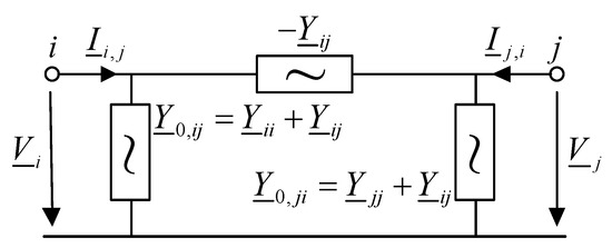
Figure 2. $\Pi$ equivalent circuit of a quadripole.

The apparent power flow ${\underline{S}}_{i,j}$ from bus i to bus j is determined by Equation (3) including the bus voltages ${\underline{V}}_i$, ${\underline{V}}_j$ and the branch admittances. Thereby, the active and reactive power flows $P_{i,j}$ and $Q_{i,j}$ in Equation (4) result in:

$$\begin{array}{cc}\hfill {\underline{S}}_{i,j}& =3V_i{\mathrm{e}}^{\mathrm{j}{\theta }_i}{\left(\left(V_i{\mathrm{e}}^{\mathrm{j}{\theta }_i}-V_j{\mathrm{e}}^{\mathrm{j}{\theta }_j}\right){\underline{Y}}_{ij}+V_i{\mathrm{e}}^{\mathrm{j}{\theta }_i}{\underline{Y}}_{0,ij}\right)}^{*}\hfill \end{array}$$

(3)

$$\begin{array}{cc}\hfill P_{i,j}& =\Re \left({\underline{S}}_{i,j}\right),Q_{i,j}=\Im \left({\underline{S}}_{i,j}\right)\hfill \end{array}$$

(4)

The vertical active $P_{\mathrm{vert}}$ and reactive power flow $Q_{\mathrm{vert}}$ result by solving Equations (3) and (4) at the interconnection buses of a higher- and lower-level grid with the respective voltage ${\underline{V}}_i$ and ${\underline{V}}_j$.

2.2. Constraints of the Optimization Problem

The solution space of the optimization problem is limited by two equality constraints based on the compliance of the power equations at each bus i [37]. In Equation (5), all power injections at bus i at a specific operating point are summarized in $P_i$ and $Q_i$. The incremental power injections $\Delta P_i$ and $\Delta Q_i$ modify the current operating point. The active and reactive power flows to connected buses j are specified by $P_{i,j}$ and $Q_{i,j}$:

$$\begin{array}{cc}\hfill 0& =P_i+\Delta P_i+\sum _j{P}_{i,j}\hfill \end{array}$$

(5)

$$\begin{array}{cc}\hfill 0& =Q_i+\Delta Q_i+\sum _j{Q}_{i,j}\hfill \end{array}$$

(6)

The technical constraints are defined by the minimum and maximum voltage limits ($V_{\min ,i},V_{\max ,i}$), the maximum thermal current limit of a line ($I_{\mathrm{th},\max ,i,j}$) and the rated load of a transformer ($S_{\mathrm{r},i,j}$), leading to following inequality constraints [21]:

$$\begin{array}{c}\hfill V_{\min ,i}\le V_i\le V_{\max ,i}\end{array}$$

(7)

$$\begin{array}{c}\hfill \left|{\left(\frac{P_{i,j}+\mathrm{j}{Q}_{i,j}}{3{\underline{V}}_i}\right)}^{*}\right|\le I_{\mathrm{th},\max ,i,j}\end{array}$$

(8)

$$\begin{array}{c}\hfill \left|{\left(\frac{P_{j,i}+\mathrm{j}{Q}_{j,i}}{3{\underline{V}}_j}\right)}^{*}\right|\le I_{\mathrm{th},\max ,i,j}\end{array}$$

(9)

$$\begin{array}{c}\hfill \sqrt{P_{i,j}^2+Q_{i,j}^2}\le S_{\mathrm{r},i,j}\end{array}$$

(10)

$$\begin{array}{c}\hfill \sqrt{P_{j,i}^2+Q_{j,i}^2}\le S_{\mathrm{r},i,j}\end{array}$$

(11)

Further inequality conditions result from the limitation of the flexibility potentials at bus i, which are based on the individual flexibilities of the different FPUs connected to this bus [21]:

$$\begin{array}{c}\hfill \Delta P_{\min ,i}\le \Delta P_i\le \Delta P_{\max ,i}\end{array}$$

(12)

$$\begin{array}{c}\hfill \Delta Q_{\min ,i}\le \Delta Q_i\le \Delta Q_{\max ,i}\end{array}$$

(13)

The flexibilities are described separately as lower and upper boundary vectors $\mathit{l}\mathit{b}$ and $\mathit{u}\mathit{b}$. Within $\mathit{l}\mathit{b}$ and $\mathit{u}\mathit{b}$, the minimum and maximum adaptation of the active and reactive power per bus i ($\Delta P_{\min ,i},\Delta P_{\max ,i},\Delta Q_{\min ,i},\Delta Q_{\max ,i}$) at the current operating point are considered.

$$\begin{array}{c}\hfill \mathit{l}\mathit{b}=\left(\Delta {\mathit{p}}_{\min },\Delta {\mathit{q}}_{\min }\right),\mathit{u}\mathit{b}=\left(\Delta {\mathit{p}}_{\max },\Delta {\mathit{q}}_{\max }\right)\end{array}$$

(14)

The optimization problem is classified as non-linear and non-convex due to the non-linear power equations as equality constraints. The non-linear optimization problem described can be directly solved in GAMS by NLP, e.g., by the IPOPT solver [22,34,35,37].

2.3. Determination of Initial Sampling Points

The solution of the optimization problem, defined by Equation (1), results in only one point on the edge of the FOR for a specific constellation of the sampling factors $\alpha$ and $\beta$. The sampling factors specified in Equation (15) guarantee the identification of the outermost edges of the FOR (see yellow area in Figure 3), which shall be sampled.

$$\begin{array}{c}\hfill \mathrm{with}(\alpha ,\beta )\in \left[(1,0),(1,1),(0,1),(-1,1),(-1,0),(-1,-1),(0,-1),(1,-1)\right]\end{array}$$

(15)

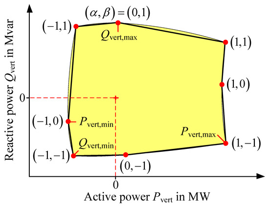
Figure 3. Example of initial sampling points of the FOR.

In Figure 3, an example for the resulting FOR based on the connection of these initial sampling points is shown. Already at the deviations of the schematic representation, it becomes clear that a sampling based on these initial points is not sufficient and detailed enough. For example, the edge between the initial points (1,0) and (1,−1) is overvalued and the edge between (0,1) and (1,1) undervalued. While an undervalued edge represents only a loss of flexibility potentials for the higher-level system operator an overvalued edge corresponds to flexibility potentials that are not existent due to limitations of the FPU or technical constraints of the lower-level grid. The premise of the FOR is the representation of guaranteed flexibility potentials and therefore an exact sampling of these non-convexities is necessary. For an appropriate sampling of the FOR, suitable sampling strategies are introduced in the following.

3. Sampling Strategies for the Determination of the FOR

Figure 4 displays four sampling strategies, differing in their respective approach to determine the FOR. The sampling strategies can be classified as angle-based (a and b) and set-point-based approaches (c and d). Each sampling strategy (except of a) is based on the previous determination of the initial sampling points by Equations (1) and (15). The sampling strategies in Figure 4 are just schematic and illustrate the general idea of the approaches and the expected results of the FOR. In order to select an appropriate sampling strategy, the four sampling strategies presented in Section 3 are compared in Section 8 regarding the quality of the results and the computation time.

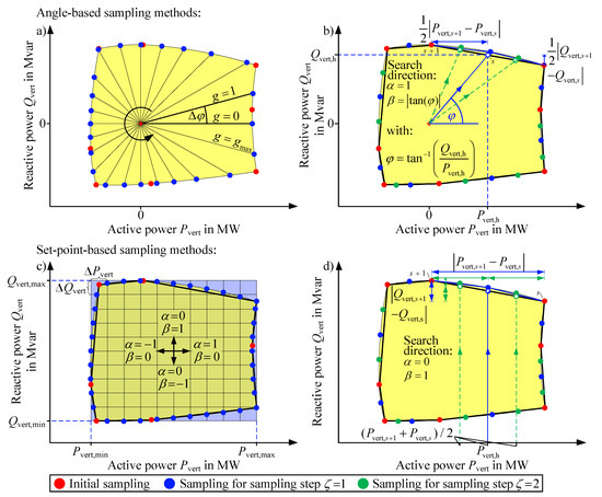
Figure 4. Sampling strategies for the determination of the FOR: (a) angle-based sampling strategy, (b) iterative angle-based sampling strategy, (c) set-point-based sampling strategy, (d) iterative set-point-based sampling strategy.

3.1. Angle-Based Sampling Strategies

The points on the edge of the FOR represent a specific relation between $P_{\mathrm{vert}}$ and $Q_{\mathrm{vert}}$ (see Figure 4a), which can be described by the angle $\phi$ [26,27]:

$$\begin{array}{c}\hfill tan\left(\phi \right)=\frac{Q_{\mathrm{vert}}}{P_{\mathrm{vert}}}=\frac{\beta }{\alpha }\end{array}$$

(16)

Dividing the unit circle by the angle sampling factor $g_{\max }$, different sampling angles $\phi$ are specified, which are used to determine the FOR for a specific constellation of $P_{\mathrm{vert}}$ and $Q_{\mathrm{vert}}$:

$$\begin{array}{c}\hfill \phi ={\phi }_0+g\Delta \phi \mathrm{with}g\le g_{\max },\Delta \phi =\frac{{360}^{\circ }}{g_{\max }}\end{array}$$

(17)

By assuming $\alpha =1$, the adapted objective function of Equation (1) for the angle-based sampling is shown in Equation (18) corresponding to Figure 4a.

$$\begin{array}{c}\hfill \min \left(F\right)=\left\{\begin{array}{c}\min \left(-P_{\mathrm{vert}}-|tan\left(\phi \right)|Q_{\mathrm{vert}}\right)\\ \min \left(P_{\mathrm{vert}}-|tan\left(\phi \right)|Q_{\mathrm{vert}}\right)\\ \min \left(P_{\mathrm{vert}}+|tan\left(\phi \right)|Q_{\mathrm{vert}}\right)\\ \min \left(-P_{\mathrm{vert}}+|tan\left(\phi \right)|Q_{\mathrm{vert}}\right)\end{array}\right.\mathrm{for}\begin{array}{c}{0}^{\circ }\le \phi <{90}^{\circ }\\ {90}^{\circ }<\phi <{180}^{\circ }\\ {180}^{\circ }\le \phi <{270}^{\circ }\\ {270}^{\circ }<\phi <{360}^{\circ }\end{array}\end{array}$$

(18)

The procedure can be parallelized by the specification of a sampling direction and using any angular resolution. An accurate sampling, using this method, is only possible for convex FOR (cf. [23]). The accuracy of the sampling also decreases with an increase in distance between the edges and the starting point (see Figure 4a). Thereby, the structure of the FOR close to the starting point is sampled in more detail than necessary. A high computation time results for a suitable sampling of the FOR.

Therefore, an iterative angle-based sampling strategy (see Figure 4b) based on the initial sampling points is introduced in [23] to obtain a sufficient approximation of the FOR within an acceptable computation time. The resulting contour determines the FOR for the initial sampling step $\zeta =0$. The distance $d_{s,s+1}$ between two neighboring sampling points s and $s+1$ (see Figure 4b) serves as convergence criterion and is determined in Equation (19) related to the values for $P_{\mathrm{vert},\min }$, $P_{\mathrm{vert},\max }$, $Q_{\mathrm{vert},\min }$, $Q_{\mathrm{vert},\max }$ (see Figure 3).

$$\begin{array}{cc}\hfill d_{s,s+1}& =\sqrt{{\left(\frac{\left|P_{\mathrm{vert},s+1}-P_{\mathrm{vert},s}\right|}{P_{\mathrm{vert},\max }-P_{\mathrm{vert},\min }}\right)}^2+{\left(\frac{\left|Q_{\mathrm{vert},s+1}-Q_{\mathrm{vert},s}\right|}{Q_{\mathrm{vert},\max }-Q_{\mathrm{vert},\min }}\right)}^2}\ge d_{\max }\hfill \end{array}$$

(19)

The iteration process continues as long as the distance $d_{s,s+1}$ between two neighboring points s and $s+1$ complies with Equation (19). The sampling can be separated regarding the number of edges so that for sampling step $\zeta =0$ a maximum of eight parallelized sampling processes can be performed. Based on the resulting sampling points, the contour of the FOR is updated for the next sampling step. The point ($P_{\mathrm{vert},\mathrm{h}}$, $Q_{\mathrm{vert},\mathrm{h}}$) on the half of the edge between two neighboring points s and $s+1$, is calculated if Equation (19) is true:

$$\begin{array}{cc}\hfill (P_{\mathrm{vert},\mathrm{h}},Q_{\mathrm{vert},\mathrm{h}})& =\left(\frac{P_{\mathrm{vert},s+1}+P_{\mathrm{vert},s}}{2},\frac{Q_{\mathrm{vert},s+1}+Q_{\mathrm{vert},s}}{2}\right)\hfill \end{array}$$

(20)

The angle ${\phi }_{s,s+1}$ and the corresponding $\beta$ are determined, considering Equation (16) and then used within an optimization based on Equation (18). The schematic sampling process is shown in Figure 4b. The computation time is reduced compared to the non-iterative angle-based sampling strategy due to the convergence criterion. If the convergence criterion is set too high, a smaller FOR can be obtained.

3.2. Set-Point-Based Sampling Strategies

A raster (see Figure 4c) is created within the basic set-point sampling strategy based on the values for $P_{\mathrm{vert},\min }$, $P_{\mathrm{vert},\max }$, $Q_{\mathrm{vert},\min }$, $Q_{\mathrm{vert},\max }$ (see Figure 3) and the dividing factor $y_{\max }$:

$$\begin{array}{c}\hfill \Delta P_{\mathrm{vert}}=\frac{\left|P_{\mathrm{vert},\min }-P_{\mathrm{vert},\max }\right|}{y_{\max }},\Delta Q_{\mathrm{vert}}=\frac{\left|Q_{\mathrm{vert},\min }-Q_{\mathrm{vert},\max }\right|}{y_{\max }}\end{array}$$

(21)

$$\begin{array}{c}\hfill P_{\mathrm{vert},\mathrm{sp}}=P_{\mathrm{vert},\min }+y\Delta P_{\mathrm{vert}},Q_{\mathrm{vert},\mathrm{sp}}=Q_{\mathrm{vert},\min }+y\Delta Q_{\mathrm{vert}},y=1,\dots ,y_{\max }\end{array}$$

(22)

The values for $P_{\mathrm{vert},\mathrm{sp}}$ specified by the raster are used to sample the top and bottom edges of the FOR (see Equation (23) whereas the values for $Q_{\mathrm{vert},\mathrm{sp}}$ are used to sample the left and the right side of the FOR (see Equation (24). The original optimization problem is extended by the compliance of the set-points $P_{\mathrm{vert},\mathrm{sp}}$ and $Q_{\mathrm{vert},\mathrm{sp}}$, respectively, as inequality constraints. The deviation factor $\kappa$ describes the permitted divergence from the set-point. The search direction (Figure 4c) is specified by the values of $\alpha$ and $\beta$ in Equation (1). The sampling process can be fully parallelized.

$$\begin{array}{c}\hfill (1-\kappa )P_{\mathrm{vert},\mathrm{sp}}\le P_{\mathrm{vert}}\le (1+\kappa )P_{\mathrm{vert},\mathrm{sp}}\end{array}$$

(23)

$$\begin{array}{c}\hfill (1-\kappa )Q_{\mathrm{vert},\mathrm{sp}}\le Q_{\mathrm{vert}}\le (1+\kappa )Q_{\mathrm{vert},\mathrm{sp}}\end{array}$$

(24)

An iterative set-point sampling strategy (see Figure 4d) is introduced in [21], using a distance-based convergence criterion to reduce the computation time while guaranteeing a detailed sampling. The convergence criterion is analogous to Equation (19) of the iterative angle-based sampling strategy. The search direction is specified by:

$$\begin{array}{c}\hfill \begin{array}{c}\mathrm{Top},\mathrm{bottom}:\\ \mathrm{Left},\mathrm{right}:\end{array}\left|P_{\mathrm{vert},s+1}-P_{\mathrm{vert},s}\right|\begin{array}{c}\ge \\ \le \end{array}\left|Q_{\mathrm{vert},s+1}-Q_{\mathrm{vert},s}\right|\end{array}$$

(25)

The inequality constraints of Equations (23) and (24) are defined by $P_{\mathrm{vert},\mathrm{sp}}=P_{\mathrm{vert},\mathrm{h}}$ (top, bottom) and $Q_{\mathrm{vert},\mathrm{sp}}=Q_{\mathrm{vert},\mathrm{h}}$ (left, right), respectively, depending on Equation (25). Furthermore, the sampling factor $\alpha$ and $\beta$ in Equation (1) are adapted based on the search direction (see Figure 4c,d). The sampling process can be parallelized like the iterative angle-based sampling strategy. Based on the general non-linear optimization problem introduced in Section 2 and the sampling strategies presented in Section 3, the optimization methods are introduced. In addition to the already mentioned solution of the NLP by the IPOPT solver in GAMS (see Section 2), the optimization problem is formulated for sequential QCLP in the next section. In Section 5, the solution of the NLP by a modified PSO is introduced.

4. Formulation of FOR Determination as Sequential Linear Constrained Quadratic Programming

Linear constrained linear programming is identified in Section 1.2 as one of the main optimization methods for the determination of the FOR. This approach achieves a fast solution by solving a linearized model of the power system under consideration of linear constraints. By approximating non-linear equations with a linear approach, inaccuracies result, which need to be taken into account, especially for a small apparent power flow within the system [38]. Considering these inaccuracies of linear constrained approaches the optimization problem is formulated as quadratically constrained linear program (see [38,39]). This optimization problem will be addressed sequentially to counteract remaining inaccuracies.

4.1. General Formulation of a Quadratically Constrained Linear Program

A general quadratically constrained linear problem is described by Equation (26)–(30), with the objective to minimize Equation (26), where $\mathit{f}$ is a vector of size mx1 and $\mathit{x}$ represents the state vector, containing the m state variables. Linear equality and inequality constraints are defined by ${\mathit{A}}_{\mathrm{eq}}$, ${\mathit{b}}_{\mathrm{eq}}$, as well as ${\mathit{A}}_{\mathrm{ineq}}$, ${\mathit{b}}_{\mathrm{ineq}}$, while the dimension of the matrices $n_{\mathrm{eq}}$xm and $n_{\mathrm{ineq}}$xm depends on the number of equality constraints $n_{\mathrm{eq}}$ and the number of inequalities constraints $n_{\mathrm{ineq}}$. The boundaries $\mathit{l}\mathit{b}$ and $\mathit{u}$ of the state variables are mx1 vectors. Quadratic constraints are defined using $\mathit{Q}$(mxm), $\mathit{l}$ (mx1) and r. The specific optimization program according to Equations (26)–(30) is described in Section 4.2.

$$\begin{array}{c}\hfill \min {\mathit{f}}^{\mathrm{T}}\mathit{x}\end{array}$$

(26)

$$\begin{array}{c}\hfill {\mathit{A}}_{\mathrm{eq}}\mathit{x}={\mathit{b}}_{\mathrm{eq}}\end{array}$$

(27)

$$\begin{array}{c}\hfill {\mathit{A}}_{\mathrm{ineq}}\mathit{x}\le {\mathit{b}}_{\mathrm{ineq}}\end{array}$$

(28)

$$\begin{array}{c}\hfill \mathit{l}\mathit{b}\le \mathit{x}\le \mathit{u}\mathit{b}\end{array}$$

(29)

$$\begin{array}{c}\hfill {\mathit{x}}^{\mathrm{T}}\mathit{Q}\mathit{x}+{\mathit{l}}^{\mathrm{T}}\mathit{x}\le \mathrm{r}\end{array}$$

(30)

4.2. Linear Objective Function with Quadratic Constraints

The active power $\Delta \mathit{p}$ and reactive power $\Delta \mathit{q}$ at each bus i of k buses are used as state variables, while $\Delta \mathit{p}$ and $\Delta \mathit{q}$ are kx1 vectors, creating a $2k$x1 vector $\mathit{x}$, shown in Equation (31).

$$\begin{array}{c}\hfill \mathit{x}={[\Delta {\mathit{p}}^{\mathrm{T}},\Delta {\mathit{q}}^{\mathrm{T}}]}^{\mathrm{T}}\end{array}$$

(31)

The objective function according to Section 2, Equation (1), is defined by Equation (32).

$$\begin{array}{c}\hfill \mathit{f}={[\underset{1\mathrm{x}k}{\underbrace{-\alpha ,0,0,\dots ,0,}}\underset{1\mathrm{x}k}{\underbrace{-\beta ,0,0,\dots ,0}}]}^{\mathrm{T}}\end{array}$$

(32)

The balance between used and generated power in the grid can be implemented by a linear equality constraint, shown in Equations (33) and (34). Linear inequality constraints are not included and therefore set to zero.

$$\begin{array}{cc}\hfill {\mathit{A}}_{\mathrm{eq}}& =\left[\begin{array}{c}{\mathit{1}}^{1\mathrm{x}k},{\mathit{0}}^{1\mathrm{x}k}\\ {\mathit{0}}^{1\mathrm{x}k},{\mathit{1}}^{1\mathrm{x}k}\end{array}\right]\hfill \end{array}$$

(33)

$$\begin{array}{cc}\hfill {\mathit{b}}_{\mathrm{eq}}& ={\mathit{0}}^{2\mathrm{x}1}\hfill \end{array}$$

(34)

$$\begin{array}{cc}\hfill {\mathit{A}}_{\mathrm{ineq}}& ={\mathit{0}}^{1\mathrm{x}k}\hfill \end{array}$$

(35)

$$\begin{array}{cc}\hfill {\mathit{b}}_{\mathrm{ineq}}& =0\hfill \end{array}$$

(36)

Additional equality constraints are included for a set-point-based sampling strategy. Therefore, Equation (37) or Equation (38) are added for sampling methods c and d and neglected for an angle-based sampling, method a and b (see Section 3.1 and Section 3.2). The index 0 represents initial values.

$$\begin{array}{c}\hfill {\mathit{a}}_{\mathrm{sp},\mathrm{p}}·\mathit{x}=[\underset{1\mathrm{x}k}{\underbrace{1,0,0,\dots ,0,}}{\mathit{0}}^{1\mathrm{x}k}]\mathit{x}=P_{\mathrm{sp}}-P_0=b_{\mathrm{eq},\mathrm{sp},\mathrm{p}}\end{array}$$

(37)

$$\begin{array}{c}\hfill {\mathit{a}}_{\mathrm{sp}},\mathrm{q}·\mathit{x}=[{\mathit{0}}^{1\mathrm{x}k},\underset{1\mathrm{x}k}{\underbrace{1,0,0,\dots ,0}}]\mathit{x}=Q_{\mathrm{sp}}-Q_0=b_{\mathrm{eq},\mathrm{sp},\mathrm{q}}\end{array}$$

(38)

The maximum and minimum adaptations of active and reactive power are limited by the flexibilities at each bus i according to Section 6, resulting in Equations (39) and (40).

$$\begin{array}{c}\hfill \mathit{u}\mathit{b}={[{\mathit{p}}_{\mathrm{flex},\mathrm{pos}}^{\mathrm{T}},{\mathit{q}}_{\mathrm{flex},\mathrm{pos}}^{\mathrm{T}}]}^{\mathrm{T}}\end{array}$$

(39)

$$\begin{array}{c}\hfill \mathit{l}\mathit{b}={[{\mathit{p}}_{\mathrm{flex},\mathrm{neg}}^{\mathrm{T}},{\mathit{q}}_{\mathrm{flex},\mathrm{neg}}^T]}^{\mathrm{T}}\end{array}$$

(40)

Quadratic inequality constraints in the form of Equation (30) are extended to Equation (41), applying Equation (42), while $\mathit{L}$ is a $(2k+T)$x$2k$ matrix, including two rows per bus i and one per terminal T. The scalar value of r is extended to the vector $\mathit{r}$. The entries of $\mathit{r}$ limit the change of the absolute values of voltages to an upper boundary and a lower boundary. The absolute values of the currents at each terminal T are only limited by an upper boundary. The Equation (10) and (11) are approximated by a maximum terminal current $i_{max}$, which is specified by $I_{\mathrm{th},\max }$ for lines and by $S_{\mathrm{r}}$ for transformers.

$$\begin{array}{c}\hfill {\mathit{x}}^{\mathrm{T}}\otimes \tilde{\mathit{Q}}\otimes \mathit{x}+\mathit{L}\mathit{x}\le \mathit{r}\end{array}$$

(41)

$$\begin{array}{c}\hfill {\mathit{x}}^{\mathrm{T}}\otimes \tilde{\mathit{Q}}\otimes \mathit{x}=\left(\begin{array}{c}{\mathit{x}}^{\mathrm{T}}{\mathit{Q}}_1\mathit{x}\\ {\mathit{x}}^{\mathrm{T}}{\mathit{Q}}_2\mathit{x}\\ ⋮\end{array}\right)\end{array}$$

(42)

The correlation of resulting voltages and currents of a power flow calculation before and after solving the optimization problem is exemplarily displayed in Equation (43) for a voltage $V_i$. Equation (43) is formulated as Equation (44) to be included in the optimization problem, shown in (45), while $\Delta v_i$ is approximated by the left side of the quadratic inequality constraint Equation (41).

$$\begin{array}{c}\hfill V_i=V_{0,i}+\Delta V_i\end{array}$$

(43)

$$\begin{array}{c}\hfill \Delta v_i={\displaystyle \frac{\Delta V_i}{V_{0,i}}}={\displaystyle \frac{V_i}{V_{0,i}}}-1={\displaystyle \frac{v_i}{v_{0,i}}}-1\end{array}$$

(44)

$$\begin{array}{c}\hfill \mathit{r}=[\underset{1\mathrm{x}k}{\underbrace{{\displaystyle \frac{v_{\max ,i}}{v_{0,i}}}-1,\dots ,}}\underset{1\mathrm{x}k}{\underbrace{{\displaystyle \frac{v_{\min ,i-k}}{v_{0,i-k}}}-1,\dots ,}}\underset{1\mathrm{x}T}{\underbrace{{\displaystyle \frac{i_{\max ,i-2k}}{i_{0,i-2k}}}-1,\dots }}{]}^{\mathrm{T}}\end{array}$$

(45)

A Taylor series of degree two is used as a quadratic approximation to represent the change of voltages and currents in regard to changes of active and reactive power. For the descriptiveness of $\mathit{Q}$ and $\mathit{L}$, the vector y is defined in Equation (46). The entries of $\mathit{L}$ are defined by Equation (47).

$$\begin{array}{cc}\hfill \mathit{y}& ={[{\mathit{p}}_k^{\mathrm{T}},{\mathit{q}}_k^{\mathrm{T}},]}^{\mathrm{T}}\hfill \end{array}$$

(46)

$$\begin{array}{cc}\hfill l_{ij}& =\left\{\begin{array}{c}{\displaystyle \frac{\partial v_i}{\partial y_j}},i\in \{1,2,\dots ,k\},j\in \{1,2,\dots ,2k\}\hfill \\ -{\displaystyle \frac{\partial v_{i-k}}{\partial y_j}},i\in \{k+1,k+2,\dots ,2k\},j\in \{1,2,\dots ,2k\}\hfill \\ {\displaystyle \frac{\partial |{\underline{I}}_{i-2k}|}{\partial y_j}},i\in \{2k+1,2k+2,\dots ,2k+T\},j\in \{1,2,\dots ,2k\}\hfill \end{array}\right.\hfill \end{array}$$

(47)

The entries $q_{p,ij}$ of a matrix ${\mathit{Q}}_p$, with $p\in \{1,2,\dots ,2k+T\}$, are defined by Equations (48)–(50).

$$\begin{array}{cc}\hfill q_{p,ij}& =\begin{array}{c}{\displaystyle \frac{1}{2}}{\displaystyle \frac{\partial v_p}{\partial y_i\partial y_j}},p\in \{1,2,\dots ,k\},i,j\in \{1,2,\dots ,k\}\hfill \end{array}\hfill \end{array}$$

(48)

$$\begin{array}{cc}\hfill q_{p,ij}& =-q_{p-k,ij},p\in \{k+1,k+2,\dots 2k\}\hfill \end{array}$$

(49)

$$\begin{array}{cc}\hfill q_{p,ij}& =\begin{array}{c}{\displaystyle \frac{1}{2}}{\displaystyle \frac{\partial |{\underline{I}}_p|}{\partial y_i\partial y_j}},p\in \{2k+1,2k+2,\dots ,2k+T\},i,j\in \{1,2,\dots ,k\}\hfill \end{array}\hfill \end{array}$$

(50)

The approximation of changes of the absolute value of voltages and currents, using a Taylor polynomial of finite order, contains inaccuracies. Therefore, the problem is solved iteratively with its previous result serving as a starting value for the next iteration step. The performance of the optimization program is highly dependent on the formulation of constraints and the objective function. While a second-order Taylor polynomial provides a better approximation than a linear constrained approach or first-order Taylor polynomial, respectively, the performance decreases. Therefore, a linear constrained approach is used for the first iterations, setting all entries in $\mathit{Q}$ to zero, providing a starting value for the QCLP. Thereafter, the QCLP is solved several times, resulting in a sequential QCLP. The results of the QCLP are checked by a power flow calculation regarding the compliance of the constraints.

5. Formulation and Modification of the Particle Swarm Optimization for the FOR Determination

Metaheuristics and especially the PSO are established in the field of electrical power supply calculations to solve various optimization problems regarding system planning and operation (see [40]). The PSO is well studied in the context of the optimal power flow determination and shows high performance and good results [30,31,32,41]. Thereby, the value of the objective function of the PSO is evaluated using a power flow calculation based on the Newton Raphson method. The results for the bus voltages ${\underline{\mathit{V}}}_i$ can be used to evaluate the objective function in Equation (1) considering the equality and inequality constraints of Section 2.2. In the following, first the iterative solution process of the classic PSO (see Section 5.1) is presented under consideration of technical constraints (see Section 5.2). Thereafter, the developed modifications regarding the FOR determination are introduced in Section 5.3. The corresponding algorithm and the parameterization for the investigations in Section 7 and Section 9 are introduced in Section 5.4.

5.1. Solution Process of the Classic Particle Swarm Optimization

The PSO adapts the swarm behavior of animals (e.g., birds foraging) to find the minimum value of the objective function based on communication and individual experience of the n swarm particles (cf. [30]). The search behavior of the swarm within the $2k$-dimensional search space is described by the $\left(n\mathrm{x}m\right)$ position and velocity matrices $\mathit{X}$ and $\mathit{V}$, where k is the number of buses. The position ${\mathit{x}}_p$ of a particle p represents a specific set of the $2k$ operational degrees of freedom within the limits of their lower boundary $\mathit{l}\mathit{b}$ and upper boundary $\mathit{u}\mathit{b}$ (see Equation (12). The velocity of a swarm particle ${\mathit{v}}_p$ describes the change of the flexibility utilization during the iterative solution process. Within the initialization step $t=1$, the particle swarm is distributed within the search space and the start velocity of the swarm particles is initialized under consideration of the start velocity factor $c_{\mathrm{v}}$. The random numbers $r_{1,p}$ and $r_{2,p}$ are uniformly distributed in the interval of $[0,1]$.

$$\begin{array}{c}\hfill {\mathit{x}}_p(t=1)=\mathit{l}\mathit{b}+r_{1,p}·(\mathit{u}\mathit{b}-\mathit{l}\mathit{b})\end{array}$$

(51)

$$\begin{array}{c}\hfill {\mathit{v}}_p(t=1)=c_{\mathrm{v}}·r_{2,p}·{\mathit{x}}_p(t=1)\end{array}$$

(52)

The values of the objective function in Equation (1) are evaluated for this initial swarm for each swarm particle by the results of a power flow calculation. The swarm particle with the best solution of Equation (1) defines the global best (index gb) position ${\mathit{x}}_{\mathrm{gb}}$ of the swarm. Additionally, the individual best (index ib) solution is determined for each particle in ${\mathit{x}}_{\mathrm{ib},p}$. For the next iteration step, each particle moves with a certain velocity ${\mathit{v}}_p$ within the search space oriented to ${\mathit{x}}_{\mathrm{gb}}$ and ${\mathit{x}}_{\mathrm{ib},p}$. Thereby, ${\mathit{x}}_{\mathrm{gb}}$ represent the social competence and ${\mathit{x}}_{\mathrm{ib},p}$ the cognitive capacity of the swarm particles:

$$\begin{array}{cc}\hfill {\mathit{v}}_p(t+1)& =i\left(t\right){\mathit{v}}_p\left(t\right)+c_1{r}_{3,p}({\mathit{x}}_{\mathrm{gb}}-{\mathit{x}}_p\left(t\right))+c_2{r}_{4,p}({\mathit{x}}_{\mathrm{ib},p}-{\mathit{x}}_p\left(t\right))\hfill \end{array}$$

(53)

$$\begin{array}{cc}\hfill {\mathit{x}}_{\mathit{p}}(t+1)& ={\mathit{x}}_p\left(t\right)+\psi ·{\mathit{v}}_p(t+1)\hfill \end{array}$$

(54)

The inertia factor $\lambda$ in Equation (55) indicates how the velocity of the swarm for the next iteration step is affected by the current velocity. The inertia decreases within the iteration process and at the beginning of the solution process a global and at the end ($t=t_{\max }$) a local search behavior of the swarm is intended.

$$\begin{array}{c}\hfill \lambda \left(t\right)={\lambda }_{\max }-t\left(\frac{{\lambda }_{\max }-{\lambda }_{\min }}{t_{\max }}\right)\end{array}$$

(55)

The random numbers $r_{3,p}$ and $r_{4,p}$ are uniformly distributed in the interval of [0,1] which characterize the stochastic nature of the PSO. The acceleration coefficients $c_1$ and $c_2$ simulate the social and the cognitive interaction within a real swarm. Both are used to calculate the constriction factor $\psi$, which ensures a convergence of the swarm in a reliable solution of the optimization problem:

$$\begin{array}{c}\hfill \psi =\frac{2}{\left|2-c-\sqrt{c^2-4c}\right|},\mathrm{with}c=c_1+c_2\ge 4\end{array}$$

(56)

The search space for the particle swarm is limited by $\mathit{lb}$ and $\mathit{ub}$ for the identification of a permissible solution (see Equation (12). If the utilization of an operational degree of freedom $q\in [1,\dots ,2k]$ of a swarm particle p is outside the limits $x_{p,q}\notin \left[l{b}_q,u{b}_q\right]$, this value is set to the respective limit value at the set-to-limit operator [42]. Based on the new swarm position $\mathit{X}(t+1)$ the objective function of the swarm is evaluated again in the next iteration step $t=t+1$. The iterative solution process stops if the maximum iteration step $t_{\max }$ is reached.

5.2. Compliance of Technical Constraints

The compliance of technical constraints is guaranteed by the punishment factor b as additional summand at the evaluation of the objective value of swarm particle p in Equation (1):

$$\begin{array}{c}\hfill F_p=-\alpha P_{\mathrm{vert},p}-\beta Q_{\mathrm{vert},p}+b_p\end{array}$$

(57)

The punishment factor needs to be determined according to the specific optimization problem in order to prevent the convergence to a local optimum [43]. In order to prevent this, a violation of the technical constraints is penalized with a smaller value at the beginning and an increased value at the end of the solution process. The punishment factor $b_p$ of a swarm particle p considers the inequality constraints of Equation (7) and is determined by:

$$\begin{array}{c}\hfill \begin{array}{cc}\hfill b_p& =\frac{1}{\left(1-\frac{(t-1)}{t_{\max }}\right)}·(\sum _i\left(\frac{V_{p,i}-V_{\max ,i}}{V_{\mathrm{r},p,i}},\forall V_{p,i}>V_{\max ,i}\right)\hfill \\ \hfill & +\sum _i\left(-\frac{V_{p,i}+V_{\min ,i}}{V_{\mathrm{r},p,i}},\forall V_{p,i}<V_{\min ,i}\right)\hfill \\ \hfill & +\sum _i\sum _j\left(\left|{\left(\frac{P_{i,j}+\mathrm{j}{Q}_{i,j}}{3{\underline{V}}_i{I}_{\mathrm{th},\max ,i,j}}\right)}^{*}\right|-1,\forall \left|{\left(\frac{P_{i,j}+\mathrm{j}{Q}_{i,j}}{3{\underline{V}}_i}\right)}^{*}\right|>I_{\mathrm{th},\max ,i,j}\right)\hfill \\ \hfill & +\sum _j\sum _i\left(\left|{\left(\frac{P_{j,i}+\mathrm{j}{Q}_{j,i}}{3{\underline{V}}_j{I}_{\mathrm{th},\max ,i,j}}\right)}^{*}\right|-1,\forall \left|{\left(\frac{P_{j,i}+\mathrm{j}{Q}_{j,i}}{3{\underline{V}}_j}\right)}^{*}\right|>I_{\mathrm{th},\max ,i,j}\right)\hfill \\ \hfill & +\sum _i\sum _j\left(\frac{\sqrt{P_{i,j}^2+Q_{i,j}^2}}{S_{\mathrm{r},i,j}}-1,\forall \sqrt{P_{i,j}^2+Q_{i,j}^2}>S_{\mathrm{r},i,j}\right)\hfill \\ \hfill & +\sum _j\sum _i\left(\frac{\sqrt{P_{j,i}^2+Q_{j,i}^2}}{S_{\mathrm{r},i,j}}-1,\forall \sqrt{P_{j,i}^2+Q_{j,i}^2}>S_{\mathrm{r},i,j}\right))\hfill \end{array}\end{array}$$

(58)

The individual summands are specified in per unit (p.u.). For example, bus voltages $V_{p,i}$ are related to the corresponding rated bus voltages $V_{\mathrm{r},p,i}$.

5.3. Modifications of the Classic Particle Swarm Optimization for an Improved FOR Determination

During the research on this article, it was identified that FORs determined by the classic PSO are significantly smaller then the results of the other optimization methods (see Section 7 Figure 5f). Two modifications of classic PSO are introduced in the following to improve the PSO regarding the FOR determination and to avoid local convergence. The convergence behavior of the modified PSO and a comparison with the results of the classic PSO are presented in Section 7.

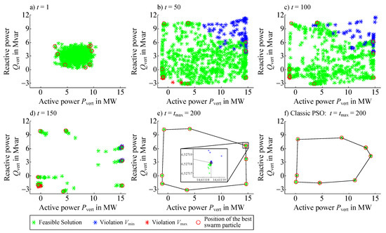
Figure 5. Convergence of the modified PSO (a–e) and comparison with the classic PSO (f).

5.3.1. Return Operator

Unpunished particles can have a worse objective function value than punished particles, due to the low punishment at the beginning of the solution process. Therefore, the swarm potentially orientates itself also at punished positions at the beginning approximating a more global result search. Thereby, unpunished particles with a good objective value are moving away from their position. Although, this result might be the best objective function value in case of a higher punishment. This may lead to a convergence to a local optimum. To retrieve the information of the best unpunished swarm particle, its position ${\mathit{x}}_{\mathrm{bu}}$ and velocity ${\mathit{v}}_{\mathrm{bu}}$ are returned to the particle swarm instead of the current worst particle specified by ${\mathit{x}}_{\mathrm{wo}}$ and ${\mathit{v}}_{\mathrm{wo}}$ at each iteration step:

$$\begin{array}{c}\hfill {\mathit{x}}_{\mathrm{wo}}={\mathit{x}}_{\mathrm{bu}},{\mathit{v}}_{\mathrm{wo}}={\mathit{v}}_{\mathrm{bu}},\mathrm{if}{\mathit{x}}_{\mathrm{bu}}\ne {\mathit{x}}_{\mathrm{gb}}\end{array}$$

(59)

5.3.2. Limitation and Inversion of Particle Velocities

The convergence behavior of the PSO is determined by the m-dimensional velocity of the swarm particles. The velocity of the particle represents the changes of the utilization of the flexibilities for the next iteration step. If the velocity $v_{p,q}$ of a certain particle is too high, the position for this flexibility utilization alternates between the limits in $l{b}_q$ and $u{b}_q$ due to the set-to-limit operator. This prevents global scanning of the permitted search space. The maximum velocities of the swarm are limited as countermeasure. The random numbers $r_{5,p,m}$ and $r_{6,p,m}$ are uniformly distributed in the interval of [0,1]:

$$\begin{array}{cc}\hfill v_{p,q}& =\frac{3}{4}{r}_{5,p,q}l{b}_q,\mathrm{if}{v}_{p,q}<\frac{3}{4}l{b}_q\wedge l{b}_q\ne 0\hfill \end{array}$$

(60)

$$\begin{array}{cc}\hfill v_{p,q}& =\frac{3}{4}{r}_{6,p,q}u{b}_q,\mathrm{if}{v}_{p,q}>\frac{3}{4}u{b}_q\wedge u{b}_q\ne 0\hfill \end{array}$$

(61)

An additional problem is caused by particle movements outside the search space. These occur especially when there are many unacceptable solutions near the global optimum. The local search for the global optimum is negatively influenced by this swarm behavior. To improve the local search of the swarm movements outside of the search space specified by the limits in $\mathit{l}\mathit{b}$ and $\mathit{u}\mathit{b}$ the velocity is inverted:

$$\begin{array}{c}\hfill v_{p,q}=-v_{p,q},\mathrm{if}\left(v_{p,q}<0\wedge x_{p,mq}=l{b}_q\right)\vee \left(v_{p,q}>0\wedge x_{p,q}=u{b}_q\right)\end{array}$$

(62)

5.4. Algorithm and Parameterization of the Modified Particle Swarm Optimization

The algorithm of the modified PSO method consists of ten steps. The solution process is based on an iterative repetition of Steps 2 to 10. The steps marked by * are the introduced modifications of the classic PSO.

Step 1: 

Initialization of the particle positions and velocities by Equation (51) at iteration step $t=1$.

Step 2: 

Evaluation of the particle swarm objective values by the objective function in Equation (1) based on the results of a power flow calculation for each swarm particle.

Step 3: 

Update of ${\mathit{x}}_{\mathrm{gb}}$ and ${\mathit{x}}_{\mathrm{ib},\mathit{p}}$.

Step 4*: 

Update of ${\mathit{x}}_{\mathrm{bu}}$ and ${\mathit{v}}_{\mathrm{bu}}$.

Step 5: 

Update of the particle velocities for the next iteration step $t=t+1$ by Equation (53).

Step 6*: 

Limitation and inversion of particle velocities by Equations (60)–(62).

Step 7: 

Update of the particle positions for the next iteration step $t=t+1$ by Equation (54).

Step 8: 

Set-to-limit operator.

Step 9*: 

Return operator.

Step 10: 

Repeat steps 2 to 10 until $t=t_{\max }$.

The parameterization of the PSO for the investigations in Section 7 and Section 9 is shown in Table 1. The need for an individual parameterization of the optimization algorithm regarding the specific optimization problem is a disadvantage of the PSO (see [44]).

Table 1. Parameterization of the PSO.

Max. Inertia ${\mathit{\lambda }}_{\mathit{max}}$	Min. Inertia ${\mathit{\lambda }}_{\mathit{min}}$	Max. Iteration ${\mathit{t}}_{\mathit{max}}$	Swarm Size n	Acceleration Coefficients ${\mathit{c}}_1,{\mathit{c}}_2$
0.9	0.4	200	100	2

6. Benchmark System and Comparison Scenario

The investigations in Section 7, Section 8 and Section 9 regarding the modifications of PSO-based FOR determination (see Section 5.3), sampling strategies (see Section 3) and optimization methods (see Section 4 and Section 5) are based on a modified version of the Cigré MV benchmark grid. This grid represents a typical European distribution system and is often used as a test grid for studies and publications in the field of DER integration. The grid variant used in the following (see Figure A1 for details) is based on the original 14-bus version [45], which is reduced by the second branch and extended by an low voltage (LV) grid level. This increases the difficulty in determining the FOR using stochastic and metaheuristic methods, since several independent operational degrees of freedom at the LV grid level influence the state variables of a single MV bus. The line lengths are extended (see Figure A1) and the tap option of the transformer at the high voltage (HV) and MV system interconnection is neglected. Thereby, the utilization of a certain amount of flexibilities of decentralized FPU may lead to operating points, violating the voltage constraints and limiting the FOR. The Cigré grid is modified regarding a high integration of converter coupled, flexible wind turbines at the MV grid level and of photovoltaic (PV) units at the LV grid level (see Figure A1). The load has no voltage dependency and was reduced as well as relocated to the LV buses. The general bus information and the results of the initial power flow results for a slack voltage of ${\underline{V}}_{i=1}=110\mathrm{kV}{\mathrm{e}}^{\mathrm{j}{0}^{\circ }}$ at the high voltage side of the HV/MV transformer are summarized in Table A3.

Operational degrees of freedom are the reduction of the energy generation of wind turbines as well as PV-units from the current operating point to zero. The reactive power supply of the wind turbines and PV-units at the reference operating point is zero. The reactive power supply can be adapted to a maximum inductive and capacitive $cos\left(\phi \right)=0.95$ for the wind turbines and $cos\left(\phi \right)=0.9$ for the PV-units [46,47]. The flexibilities are defined separately for the MV and LV grid level and individually for each kind of FPU connected to bus i. The change of the operating point of an FPU ($\Delta P_i$, $\Delta Q_i$) is limited by the maximum apparent power $S_{\max ,i}$ according to Equation (65).

$$\begin{array}{cc}\hfill \mathrm{MV}:& \begin{array}{c}\Delta P_{\min ,i}=0,\Delta P_{\max ,i}=-P_{\mathrm{wind},i},\hfill \\ \Delta Q_{\min ,i},\Delta Q_{\max ,i}=\pm P_{\mathrm{wind},i}\frac{sin\left({\cos }^{-1}\left(0.95\right)\right)}{0.95}\hfill \end{array}\hfill \end{array}$$

(63)

$$\begin{array}{cc}\hfill \mathrm{LV}:& \begin{array}{c}\Delta P_{\min ,i}=0,\Delta P_{\max ,i}=-P_{\mathrm{PV},i},\hfill \\ \Delta Q_{\min ,i},\Delta Q_{\max ,i}=\pm P_{\mathrm{PV},i}\frac{sin\left({\cos }^{-1}\left(0.9\right)\right)}{0.9}\hfill \end{array}\hfill \end{array}$$

(64)

$$\begin{array}{c}\hfill S_{\max ,i}=\sqrt{{(P_i+\Delta P_{\mathrm{i}})}^2+{(Q_i+\Delta Q_{\mathrm{i}})}^2}\end{array}$$

(65)

The maximum loading of the transformers $S_{\mathrm{r}}$ and the maximum thermal current limit of a line $I_{\mathrm{th},\max }$ are displayed in Table A1 and Table A2 (Appendix A). The limits for the minimum and the maximum voltage are $V_{\min ,i}=0.9V_{\mathrm{r},i}$ and $V_{\max ,i}=1.1V_{\mathrm{r},i}$, respectively. A fully described and more detailed data set (e.g., including the vectors $\mathit{u}\mathit{b}$ and $\mathit{l}\mathit{b}$) is available at [48].

7. Convergence Behavior of the Modified Particle Swarm Optimization

The improved convergence of the modified PSO is exemplary shown for the determination of eight initial sampling points of Equation (15). Each sampling point is considered at Equation (1) and an individual modified PSO run is started. The process of FOR determination is repeated five times for the classic and the modified PSO due to their stochastic nature and possible local convergence. In the following, just the results of the best runs are considered. Figure 5a–e show the convergence behavior of the eight corresponding particle swarms. The results from the final iteration step are shown in Figure 5e. In Figure 5f, the results of the classic PSO are shown to illustrate the advantages of the PSO adaptations.

The eight initial swarms at iteration step $t=1$ are gathered in the middle of the PQ-plane. This folding problem is based on the central limit theorem of the probability theory [16], which also occurs at the stochastic approaches for the FOR determination (cf. [15,17]). The particles with the best solution (see red circles in Figure 5a) are already orientated to the corresponding edges of the FOR. During the solution process, the particle swarm moves through the PQ-plane searching for a new ${\mathit{x}}_{\mathrm{gb}}$. Thereby the solution search becomes increasingly local. Within the solution process a variety of particles with a violation of the voltage limits occur especially at areas with a high, uniformly directed $P_{\mathrm{vert}}$ and $Q_{\mathrm{vert}}$, respectively, to the lower-level grid. For sampling points in these areas the swarm does not converge in a uniform result (see close up in Figure 5e). This leads to small deviations of the FOR at each run of the modified PSO. The modifications of the PSO lead to significantly better results for all sampling points. For example the deviations of the upper left sampling points are $\Delta P_{\mathrm{vert}}=-1.10\mathrm{MW}$ and $\Delta Q_{\mathrm{vert}}=2.13\mathrm{Mvar}$. The area of the FOR in Figure 5f is $34.07\%$ smaller than in Figure 5e).

8. Comparison of FOR Sampling Strategies

A scattered polygonal area of 5000 FOR sampling points ($y_{\max }=1250$, see Equation (21) serves as a basis for the comparison. The area $A_{\mathrm{sp},5000}$ is the result of the NLP solved in GAMS. The quality of the results is evaluated under consideration of the area factor $\Delta A$ in Equation (66) and the sampling of non-convexities. Thereby, the convex hull of the FOR (see red dotted line in Figure 6a) is used for the determination of non-convexities. The non-convexities occur in regions where the FOR is not limited by the constraints of the operational degrees of freedom but by violations of the voltage limits (cf. Figure 5b,c).

$$\begin{array}{c}\hfill \Delta A=\frac{A-A_{\mathrm{sp},5000}}{A_{\mathrm{sp},5000}}\end{array}$$

(66)

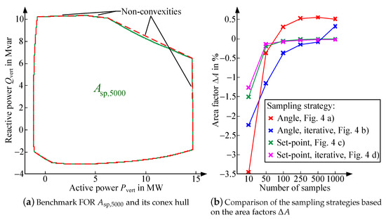
Figure 6. Comparison of the optimization methods for the FOR determination.

The sampling of the FOR becomes more detailed with an increasing number of sampling points. Thereby, the deviations of the individual FOR from $A_{\mathrm{sp},5000}$ decreases and the area factor $\Delta A$ increases (see Figure 6b). The set-point sampling strategies approximate $A_{\mathrm{sp},5000}$ already with 100 samples (see green course in Figure 6b). A more detailed sampling of the non-convexities leads to a reduction of the FOR while the other edges are simultaneously sampled in more detail, which results in an enlargement of the FOR. Thereby, a significant reduction of the deviation takes a high number of samples. The advantage of the iterative set-point sampling strategy is the consideration of the convergence criterium in Equation (19), which leads to appropriate results and a reduction of the computation time, independent from the investigated grid scenario. The convergence criterium (here: $d_{\max }=0.001$) is reached after 128 samples, which results in a suitable FOR determination with an area factor of $\Delta A=0.03\%$.

The angle-based approaches do not identify the non-convexities of the FOR. The area of the angle-based sampling strategy $A_{\mathrm{a},500}$ for a number of 500 samples corresponds to the convex hull in Figure 6a. The identification of non-convexities occurs rarely and only with a high sampling resolution $g_{\max }$. This leads to a smaller area factor $\Delta A$ at the angle-based approach comparing the FOR areas for a number of 500 and 1000 samples. The iterative set-point-based sampling strategy of Figure 4 d with a $d_{\max }$ equal to 0.001 is used in the following for the comparison of the optimization methods.

9. Comparison of the Optimization Methods Regarding the FOR Determination

The results of the different optimization methods, using iterative set-point sampling, are presented in Figure 7a and compared to the benchmark FOR $A_{\mathrm{sp},5000}$. All results represent valid operating points of the grid with no violation of the technical constraints (see Section 2.2). In general, the iterative sampling leads to an appropriate FOR determination (cf. red and green lines). A significant deviation from $A_{\mathrm{sp},5000}$ only results at the lower left edge and the right side of the FOR. The deviations at the lower left edge can be explained by reaching the convergence criterium $d_{\max }$ before sampling the edge (also applies to the PSO). The deviations at the right side are based on a local convergence of the IPOPT solver in GAMS.

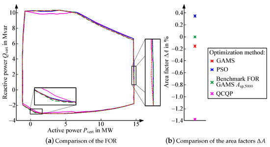
Figure 7. Comparison of the optimization methods for the FOR determination.

The results from the QCLP provide the smallest FOR with significant deviations from the benchmark FOR and a negative area factor in Figure 7b. The QCLP has disadvantages in sampling the FOR in regions near the violation of the upper voltage constraint (see left bottom in Figure 7a. In contrast, the QCLP has advantages in sampling regions where a compliance of the lower voltage limit is difficult. Thereby, the QCLP has the broadest edges at the right top of Figure 7a. The deviations at the left top are based on the dependence of the active and reactive power demand of the grid from active and reactive power variations by the FPU. This approximately quadratic behavior also occurs at the solution process of the modified PSO, shown in Figure 8. The number of particles was increased to display this phenomenon. The swarm finds PQ-constellations of the FPU which leads to better final results (see Figure 7a) during the convergence process. The remaining deviations at the left top are based on local convergences and can be eliminated by an increase of the PSO runs. Further investigations regarding the QCLP are required for a more accurate sampling of the left top.

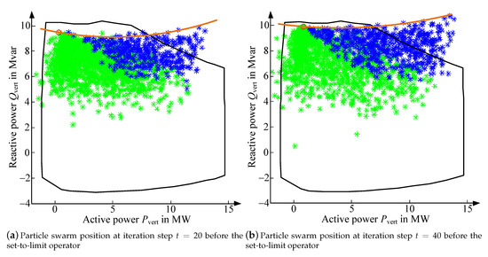
Figure 8. Convergence of the PSO for sampling set-point of $P_{\mathrm{vert},\mathrm{sp}}=1.5\mathrm{MW}$ and $\alpha =0,\beta =1$.

The modified PSO finds better results than GAMS for the top right edge of the FOR analogously to the QCLP. Small deviations from the benchmark FOR occur at the lower left edge because of local convergence. Based on the area factor (see Figure 7b) the PSO provides the largest FOR. The computation time for the optimization methods is shown in Table 2.

Table 2. Computation time of the different optimization methods.

GAMS	Modified PSO	Benchmark FOR GAMS ${\mathit{A}}_{\mathit{sp},5000}$	QCLP
105 s	640 s	10910 s	164 s

These results only show tendencies between the optimization methods. All simulations were executed on a system with a 2.6 GHz quad core processor and 16 GB local storage. The preparation of the input variables to the optimizers is done uniformly in MathWorks MATLAB R2019b. The modified PSO is fully implemented in MATLAB while the NLP is solved by the IPOPT solver of the commercial software GAMS. The Taylor polynomials for the first and second derivations of the power equations at the QCLP are set up in MATLAB and solved using the OptiToolbox. None of the methods were parallelized.

10. Discussion

In general, the development of new sampling strategies should focus on a reduction of the required number of samples, while maintaining the same quality of results. The iterative set-point-based sampling leads to appropriate results while reducing the computation time significantly. A more detailed sampling of the FOR is possible by a simple adjustment of the convergence criterion. For this reason, the iterative set-point-based sampling was selected for the comparison of the optimization methods in Section 9. The set-point-based sampling strategies provide a larger FOR compared to the angle-based approaches (see Section 8). Additionally, the FOR is sampled in more detail and non-convexities are identified appropriately. The reason for this is the consideration of the angle specifications as sampling factors at the objective function (see Equation (18) instead of a defined constraint in the set-point-based sampling strategies. A trade-off between the compliance of the angle specification and the minimization of the sum of $P_{\mathrm{vert}}$ and $Q_{\mathrm{vert}}$ (see Equation (18) results from angle-based sampling. A pareto optimal set results for the solution of the objective function. To cope with the sampling of non-convexities by angle-based sampling strategies, the compliance of the angle ${\phi }_{\mathrm{sp}}$ needs to be included as a constraint of the optimization problem in future investigations:

$$\begin{array}{c}\hfill {\phi }_{\mathrm{sp}}={tan}^{-1}\left(\frac{Q_{\mathrm{vert}}}{P_{\mathrm{vert}}}\right)\end{array}$$

(67)

A detailed sampling of the non-convexities is important because deviations represent a over-, respectively under-, estimation of the lower-level flexibility potential. Especially, an overestimation can lead to critical situations because the higher-level system operator assumes guaranteed potentials. The deviation from the non-convex FOR to its convex hull depends on the specific grid scenario (e.g., grid structure, relation between power supply and consumption at the specific operating point). A convex hull can be generated around the point cloud for the determination of a convex FOR. In contrast, the exact position of a new sampling point on the edge of the FOR needs to be known to identify and describe non-convexities. This could be achieved by the definition of a sample direction or by the knowledge of the neighboring sampling points at iterative approaches. The influencing factors on the non-convexity of an FOR need to be investigated in more detail in future work.

The solution process of GAMS requires the lowest computation time comparing the results in Table 2. The preparation time to create the Taylor polynomials for the QCLP varies on the grid size and can take a large portion of the computation time while the solution time is negligible. Therefore, large grid sizes of a few hundred buses might not be suitable for this approach. The computation time of the iterative solution process of the PSO only depends on the amount of power flow calculations per sampling point. An increase of the swarm size or the termination criteria leads to an increase of the computation time. In contrast, an adaptation of the objective function by additional evaluation criteria or the consideration of more complex constraints has no significant influence. Especially for the PSO the implementation of more robust and effective load flow calculation methods considering the individual characteristics of the specific grid level is an interesting research aspect (see [49]). Note that variations of the optimization problem (e.g., different sampling sizes, inclusion of tap positions of OLTC transformers) might vary in their impact, depending on the used approach. Therefore, Table 2 gives an overview, but not a complete evaluation of the computation times of the optimization methods.

The classic PSO is not a suitable aggregation method comparing the eight initial sampling points from the classic PSO (see Section 7) with the results of the NLP and the QCLP (see Section 9). The introduced modifications of the PSO prevent fast local convergence and lead to a significant improvement of the convergence behavior (see Section 7). Thereby the modified PSO is identified as the most suitable optimization-based FOR determination method regarding the size of the FOR and the sampling of non-convexities (see Section 9). There are different demands on the quality of the result or the computation time depending on the use of the FOR. Exemplarily, less accurate methods are recommended (e.g., solution of the NLP by the IPOPT solver in GAMS) for neglectable non-convexities and the need of a fast solution. The general focus needs to be the improvement of the different optimization methods regarding a more detailed FOR determination for their respective fields of application (e.g., consideration of mixed-integer flexibilities at the QCLP, optimized parameterization of the PSO, increase of PSO runs to avoid local convergence). When interpreting the results, it has to be considered that the simulations are based on a single investigation scenario and therefore not to be regarded as generally valid. Nevertheless, the given survey on aggregation methods for the determination of the flexibility potentials at the TSO/DSO and DSO/DSO interfaces as well as the investigations and results of this article provide a basis for further investigations regarding various research aspects.

The consideration of a non-convex FOR results in piece wise linear constraints for the NLP. In addition to a more complex description of the optimization problem, this may lead to local convergences and higher computation times for the solution by the IPOPT solver in GAMS or the QCLP approach. In contrast, the quality of the results and the computation time of the PSO and other population based metaheuristics is related to the number of operational degrees of freedom and the grid size. The compliance of FPU or FOR constraints, described as a polygonal area, can be guaranteed by the adaptation of the set-to-limit operator by the polygon theorem according to Jordan. The PSO provides additional meta information, such as the costs for a certain adjustment of the vertical active and reactive power exchange. Further advantages of the PSO are the simple implementation of any optimization target by a modular objective function, the consideration of non-linear constraints and mixed-integer degrees of freedom, as well as the scaling properties regarding grid size and the number and limits of the degrees of freedom.

The investigations of this paper can be repeated for the mixed integer NLP based on a more detailed flexibility description. The flexibility area of the FPU is represented by a square at the PQ-plane (see Equation (14). Thereby, dependencies between $\Delta P$ and $\Delta Q$ are neglected for the adaptation of the current operating point. Specifications according to the technical grid connection guidelines are polygonal and sometimes non-convex areas [46,47]. The consideration of a convex FPU flexibility is possible for each of the presented optimization methods by linear constraints. The consideration of flexibilities, e.g., OLTC transformer tap sets, switching operations, can also be included resulting in a mixed integer NLP.

The TSO/DSO and DSO/DSO interfaces need to be considered together for investigations regarding the potentials of vertical grid control concepts in a multi-voltage-level context to guarantee safe and reliable energy supply. In contrast, the FOR is determined either for the TSO/DSO or the DSO/DSO interface in literature, as well as in this paper. Therefore, a method for a cascading FOR determination from the lower to the higher voltage levels needs to be developed and the resulting flexibility potentials integrated at the operational management of the individual system operators.

Another important aspect in future research is the consideration of multiple interfaces between two system operators (cf. [12,14]). This represents a more realistic grid scenario, especially for the TSO/DSO interface, and is neglected in current literature. Therefore, the distribution of a certain flexibility request from the TSO to the individual TSO/DSO interfaces needs to be examined in more detail. As a starting point, sensitivity analyses of the vertical power flows depending on the distributed flexibility utilization can be performed to evaluate the interdependence of vertical power flows.

In future investigations, the PSO approach will be compared with other population-based metaheurstics, in particular algorithms such as the covariance matrix adaptation evolution strategy (CMA-ES) [50] and an evolutionary training algorithm for artificial neural networks (REvol) [51]. Furthermore, it will be investigated if the total number of required objective function evaluations can be reduced when sampling the border of the FOR in one run by dynamically adapting the underlying objective function, which is possible with population-based approaches. Different investigation scenarios based on larger or real grid structures need to be investigated for further comparisons of the optimization methods and the proof of the general validity of the results. Uncertainties at the FOR determination can be considered to determine the flexibility potentials (resistance to reactance ratio, variations of the slack voltages at the vertical interconnection busses, operating points and voltage dependency of the loads). Especially regarding the day-ahead or intraday planning of the system, operation forecast deviations for the renewables are important (cf. [17]). In addition, ramp times or time delays for a certain flexibility provision can be taken into account (cf. [19]).

11. Conclusions

This article provides a survey on state-of-the-art aggregation methods for the determination of a feasible operation region (FOR) at the vertical system interfaces. The advantages of optimization-based aggregation methods compared to stochastic approaches are identified. Within this article three optimization methods for the determination of the FOR are compared for the first time. In particular, these are non-linear programming, sequential quadratically constrained linear programming and a newly developed, modified particle swarm optimization (PSO). A main component of optimization-based aggregation methods is the sampling strategy. In literature, different angle- and set-point-based sampling strategies are discussed. Before the comparison of the optimization methods four sampling strategies are compared for the non-linear programming. The iterative set-point-based sampling strategy enables a specification of the requested level of detail of the FOR by specifying of a convergence criterion. This results in an appropriate sampling of the FOR, while guaranteeing the compliance of technical constraints. Furthermore, the computation time is reduced compared to same level of detail at the non-iterative set-point-based approach. The modifications of the PSO avoid local convergence and lead to significant improvements regarding the determination of the FOR compared to the classic PSO. The three optimization methods were compared regarding the computation time, the size of the FOR based on the area factor and the sampling of non-convexities. In general, each of the investigated optimization methods can be used for the determination of the FOR according to the quality of the results. The selection of an optimization method depends on the specific case of application. The developed modified PSO achieves the best results regarding the size of the FOR and the sampling of non-convexities. The PSO is competitive with the two main categories of optimization-based FOR determination methods from the literature. Improving the computation time and considering the expected advantages with respect to an integration of the approach into a hierarchical grid control concept represent significant potentials.

References

- Hillberg, E.; Zegers, A.; Herndler, B.; Wong, S.; Pompee, J.; Bourmaud, J.Y.; Lehnhoff, S.; Migliavacca, G.; Uhlen, K.; Oleinikova, I. Flexibility Needs in the Future Power System; ISGAN: Washington, DC, USA, 2019. [Google Scholar]
- Zegers, A.; Brunner, H. TSO-DSO interaction: An Overview of current interaction between transmission and distribution system operators and an assessment of their cooperation in Smart Grids. In International Smart Grid Action Network (ISAGN) Discussion Paper Annex; ISGAN: Washington, DC, USA, 2014; Volume 6. [Google Scholar]
- Gerard, H.; Rivero, E.; Six, D. Basic schemes for TSO-DSO coordination and ancillary services provision. SmartNet Deliv. D 2016, 1, 3. [Google Scholar]
- ENTSO-E. General Guidelines or Reinforcing the Cooperation between TSO and DSO; ENTSO-E: Brussels, Belgium, 2015. [Google Scholar]
- ENTSO-E. Towards Smarter Grids: Developing TSO and DSO Roles and Interactions for the Benefit of Consumers; Technical Report; ENTSO-E: Brussels, Belgium, 2015. [Google Scholar]
- ENTSO-E. Distributed Flexibility and the Value of TSO/DSO Cooperation; ENTSO-E: Brussels, Belgium, 2017. [Google Scholar]
- ENTSO-E. TSO-DSO Report—An Integrated Approach to Active System Management with the Focus on TSO-DSO Coordination in Congestion Management and Balancing; ENTSO-E: Brussels, Belgium, 2019. [Google Scholar]
- ENTSO-E. Distributed Flexibility and the Value of TSO/DSO Cooperation; ENTSO-E: Brussels, Belgium, 2016. [Google Scholar]
- Power, M.; Roggatz, C.; Norlander, C.; Diskin, E.; Power, S.; Kranhold, M.; Probst, A.; Belhomme, R.; Bose, A.; Gaudin, J.; et al. Cigré-733-System Operation Emphasizing DSO/TSO Interaction and Coordination; Cigré Technical Brochures; Study Committee: C2, C6; Working Group: JWG C2/C6.36; CIGRE- International Council on large Electric Systems: Paris, France, 2018. [Google Scholar]
- Han, X.; Heussen, K.; Gehrke, O.; Bindner, H.W.; Kroposki, B. Taxonomy for Evaluation of Distributed Control Strategies for Distributed Energy Resources. IEEE Trans. Smart Grid 2018, 9, 5185–5195. [Google Scholar] [CrossRef]
- Givisiez, A.G.; Petrou, K.; Ochoa, L.F. A Review on TSO-DSO Coordination Models and Solution Techniques. Electr. Power Syst. Res. 2020, 189, 106659. [Google Scholar] [CrossRef]
- Westermann, D.; Wolter, M.; Komarnicki, P.; Schlegel, S.; Schwerdfeger, R.; Richter, A.; Arendarski, B. Control strategies for a fully RES based power system. In Proceedings of the International ETG Congress 2017, Bonn, Germany, 28–29 November 2017; pp. 1–6. [Google Scholar]
- Sarstedt, M.; Kluß, L.; Dokus, M.; Hofmann, L.; Gerster, J. Simulation of Hierarchical Multi-Level Grid Control Strategies. In Proceedings of the IEEE International Conference on Smart Grids and Energy Systems, Perth, Australia, 23–26 November 2020; p. 6. [Google Scholar]
- Schwerdfeger, R.; Schlegel, S.; Westermann, D.; Lutter, M.; Junghans, M. Methodology for Next Generation System Operation between DSO and DSO; CIGRE: Paris, France, 2016; pp. 1–9. [Google Scholar]
- Heleno, M.; Soares, R.; Sumaili, J.; Bessa, R.; Seca, L.; Matos, M.A. Estimation of the Flexibility Range in the Transmission-Distribution Boundary. In Proceedings of the 2015 IEEE Eindhoven PowerTech, Eindhoven, The Netherlands, 29 June–2 July 2015; pp. 1–6. [Google Scholar]
- Landau, D.P.; Binder, K. A Guide to Monte Carlo Simulations in Statistical Physics; Cambridge University Press: Cambridge, UK, 2014. [Google Scholar]
- Mayorga Gonzalez, D.; Hachenberger, J.; Hinker, J.; Rewald, F.; Hager, U.; Rehtanz, C.; Myrzik, J. Determination of the Time-Dependent Flexibility of Active Distribution Networks to Control Their TSO-DSO Interconnection Power Flow. In Proceedings of the 2018 Power Systems Computation Conference (PSCC), Dublin, Ireland, 11–15 June 2018; pp. 1–8. [Google Scholar]
- Ageeva, L.; Majidi, M.; Pozo, D. Analysis of feasibility region of active distribution networks. In Proceedings of the 2019 IEEE International Youth Conference on Radio Electronics, Electrical and Power Engineering (REEPE), Moscow, Russia, 14–15 March 2019; pp. 1–5. [Google Scholar]
- Riaz, S.; Mancarella, P. On Feasibility and Flexibility Operating Regions of Virtual Power Plants and TSO/DSO Interfaces. In Proceedings of the 2019 IEEE Milan PowerTech, Milan, Italy, 23–27 June 2019; pp. 1–6. [Google Scholar]
- Fonseca, N.; Silva, J.; Silva, A.; Sumaili, J.; Seca, L.; Bessa, R.; Pereira, J.; Matos, M.; Matos, P.; Morais, A.C.; et al. EvolvDSO Grid Management Tools to Support TSO-DSO Cooperation; CIRED Workshop: Paris, France, 2016; pp. 1–4. [Google Scholar]
- Silva, J.; Sumaili, J.; Bessa, R.J.; Seca, L.; Matos, M.A.; Miranda, V.; Caujolle, M.; Goncer, B.; Sebastian-Viana, M. Estimating the Active and Reactive Power Flexibility Area at the TSO-DSO Interface. IEEE Trans. Power Syst. 2018, 33, 4741–4750. [Google Scholar] [CrossRef]
- Capitanescu, F. TSO–DSO Interaction: Active Distribution Network Power Chart for TSO Ancillary Services Provision. Electr. Power Syst. Res. 2018, 163, 226–230. [Google Scholar] [CrossRef]
- Contreras, D.A.; Rudion, K. Improved Assessment of the Flexibility Range of Distribution Grids Using Linear Optimization. In Proceedings of the 2018 Power Systems Computation Conference (PSCC), Dublin, Ireland, 11–15 June 2018. [Google Scholar]
- Contreras, D.; Laribi, O.; Banka, M.; Rudion, K. Assessing the Flexibility Provision of Microgrids in MV Distribution Grids; CIRED Workshop: Paris, France, 2018. [Google Scholar]
- Contreras, D.A.; Rudion, K. Impact of Grid Topology and Tap Position Changes on the Flexibility Provision from Distribution Grids. In Proceedings of the 2019 IEEE PES Innovative Smart Grid Technologies Europe (ISGT-Europe), Bucharest, Romania, 29 September–2 October 2019; pp. 1–5. [Google Scholar]
- Rossi, M.; Viganò, G.; Moneta, D.; Vespucci, M.T.; Pisciella, P. Fast estimation of equivalent capability for active distribution networks. CIRED-Open Access Proc. J. 2017, 2017, 1763–1767. [Google Scholar] [CrossRef]
- Viganò, G.; Rossi, M.; Moneta, D. Effects of Distribution System Characteristics on TSO-DSO Ancillary Services Exchange; CIRED Workshop: Paris, France, 2019. [Google Scholar]
- Fortenbacher, P.; Demiray, T. Reduced and Aggregated Distribution Grid Representations Approximated by Polyhedral Sets. arXiv 2019, arXiv:1903.07549. [Google Scholar] [CrossRef]
- Stanković, S.; Söder, L.; Hagemann, Z.; Rehtanz, C. Reactive Power Support Adequacy at the DSO/TSO Interface. Electr. Power Syst. Res. 2020, 190, 106661. [Google Scholar] [CrossRef]
- Optimal Power Flow. In Optimization of Power System Operation; John Wiley & Sons, Ltd.: Hoboken, NJ, USA, 2015; Chapter 8; pp. 297–364. [CrossRef]
- Abido, M.A. Optimal power flow using particle swarm optimization. Int. J. Electr. Power Energy Syst. 2002, 24, 563–571. [Google Scholar] [CrossRef]
- Sharma, T.; Yadav, A.; Jamhoria, S.; Chaturvedi, R. Comparative study of methods for optimal reactive power dispatch. Electr. Electron. Eng. 2014, 3, 53–61. [Google Scholar] [CrossRef]
- Frank, S.; Rebennack, S. An introduction to optimal power flow: Theory, formulation, and examples. IIE Trans. 2016, 48, 1172–1197. [Google Scholar] [CrossRef]
- Stock, D.S.; Venzke, A.; Löwer, L.; Rohrig, K.; Hofmann, L. Optimal reactive power management for transmission connected distribution grid with wind farms. In Proceedings of the 2016 IEEE Innovative Smart Grid Technologies–Asia (ISGT-Asia), Melbourne, Australia, 28 November–1 December 2016; pp. 1076–1082. [Google Scholar] [CrossRef]
- Stock, D.S.; Sala, F.; Berizzi, A.; Hofmann, L. Optimal control of wind farms for coordinated TSO-DSO reactive power management. Energies 2018, 11, 173. [Google Scholar] [CrossRef]
- Kundur, P.; Balu, N.J.; Lauby, M.G. Power System Stability and Control; McGraw-Hill: New York, NY, USA, 1994; Volume 7. [Google Scholar]
- Soroudi, A. Power System Optimization Modeling in GAMS; Springer: Berlin, Germany, 2017; Volume 78. [Google Scholar]
- Leveringhaus, T.; Hofmann, L. Combined and optimized redispatch management of multiple congestions and voltage deviations with active and reactive power based on AC-PTDFs with distributed slack. In Proceedings of the 2015 IEEE Power Energy Society General Meeting, Denver, CO, USA, 26–30 July 2015; pp. 1–5. [Google Scholar] [CrossRef]
- Leveringhaus, T.; Hofmann, L. Optimal power flow comprising congestions and voltage management by global quadratic optimization of active and reactive power. In Proceedings of the 2016 IEEE International Conference on Power System Technology (POWERCON), Wollongong, Australia, 28 September–1 October 2016; pp. 1–6. [Google Scholar] [CrossRef]
- Working Group on Modern Heuristic Optimization (WGMHO) under the IEEE PES Analytic Methods in Power Systems (AMPS) Committee. Available online: https://site.ieee.org/psace-mho/ (accessed on 28 January 2021).
- Sarstedt, M.; Garske, S.; Hofmann, L. Application of PSO-Methods for the Solution of the economic Optimal Reactive Power Dispatch Problem. In Proceedings of the 2018 IEEE Electronic Power Grid (eGrid), Charleston, SC, USA, 12–14 November 2018; pp. 1–6. [Google Scholar] [CrossRef]
- Zhao, B.; Guo, C.; Cao, Y. A multiagent-based particle swarm optimization approach for optimal reactive power dispatch. IEEE Trans. Power Syst. 2005, 20, 1070–1078. [Google Scholar] [CrossRef]
- Coath, G.; Halgamuge, S.K. A comparison of constraint-handling methods for the application of particle swarm optimization to constrained nonlinear optimization problems. In Proceedings of the IEEE 2003 Congress on Evolutionary Computation, Canberra, Australia, 8–12 December 2003; Volume 4, pp. 2419–2425. [Google Scholar]
- Sennewald, T.; Linke, F.; Reck, J.; Westermann, D. Parameter Optimization of Differential Evolution and Particle Swarm Optimization in the Context of Optimal Power Flow. In Proceedings of the 2020 IEEE PES Innovative Smart Grid Technologies Europe (ISGT-Europe), Delft, The Netherlands, 26–28 October 2020; pp. 1045–1049. [Google Scholar] [CrossRef]
- Rudion, K.; Orths, A.; Styczynski, Z.A.; Strunz, K. Design of benchmark of medium voltage distribution network for investigation of DG integration. In Proceedings of the IEEE Power Engineering Society General Meeting, Montreal, QC, Canada, 18–22 June 2006. [Google Scholar]
- VDE-Application Rule: VDE-AR-N 4105: 2018-11 Power Generating Plants in the Low Voltage Grid; VDE: Berlin, Germany, 2018.
- VDE-Application Rule: VDE-AR-N 4110: 2018-11 Technical Connection Rules for Medium-Voltage; VDE: Berlin, Germany, 2018.
- Marcel, S.; Neelotpal, M.; Christoph, B.; Lutz, H. Dataset: Multi-Voltage-Level Electric Power System Data Sets—Survey and Comparison of Optimization-Based Aggregation Methods for the Determination of the Flexibility Potentials at Vertical System Interconnections; Leibniz University Hannover: Hannover, Germany, 2020. [Google Scholar] [CrossRef]
- Parizad, A.; Hatziadoniu, K. Security/stability-based Pareto optimal solution for distribution networks planning implementing NSGAII/FDMT. Energy 2020, 192, 116644. [Google Scholar] [CrossRef]
- Hansen, N. The CMA evolution strategy: A comparing review. In Towards a New Evolutionary Computation. Advances on Estimation of Distribution Algorithms; Lozano, J., Larranaga, P., Inza, I., Bengoetxea, E., Eds.; Springer: Berlin, Germany, 2006; pp. 75–102. [Google Scholar]
- Veith, E.; Ruppert, M.; Steinbach, B. An Evolutionary Training Algorithm for Artificial Neural Networks with Dynamic Offspring Spread and Implicit Gradient Information; IARIA: Porto, Portugal, 2014. [Google Scholar]
Publisher’s Note: MDPI stays neutral with regard to jurisdictional claims in published maps and institutional affiliations. |
© 2021 by the authors. Licensee MDPI, Basel, Switzerland. This article is an open access article distributed under the terms and conditions of the Creative Commons Attribution (CC BY) license (http://creativecommons.org/licenses/by/4.0/).