Article

ELM-QR-Based Nonparametric Probabilistic Prediction Method for Wind Power

1
Key Laboratory of Energy Thermal Conversion and Control of Ministry of Education, School of Energy and Environment, Southeast University, Nanjing 210096, China
2
Nanjing NARI-RELAYS Electric Co. Ltd., Nanjing 211102, China
*
Author to whom correspondence should be addressed.
Energies 2021, 14(3), 701; https://doi.org/10.3390/en14030701
Submission received: 5 January 2021 / Revised: 21 January 2021 / Accepted: 26 January 2021 / Published: 29 January 2021
(This article belongs to the Section A3: Wind, Wave and Tidal Energy)

Abstract

:
Wind power has significant randomness. Probabilistic prediction of wind power is necessary to solve the problem of safe and stable power grid dispatching with the integration of large-scale wind power. Therefore, this paper proposes a novel nonparametric probabilistic prediction model for wind power based on extreme learning machine-quantile regression (ELM-QR). Firstly, the ELM-QR models of multiple quantiles are established, and then the new comprehensive index (NCI) is optimized by particle swarm optimization (PSO) to obtain the weighting coefficients corresponding to the lower and upper bounds of the prediction intervals. The final prediction interval is obtained by integrating the outputs of ELM-QR models and the weighting coefficients. Finally, case studies are carried out with the real wind farm operation data, simulation results show that the proposed algorithm can obtain narrower prediction intervals while ensuring high reliability. Through sensitivity analysis and comparison with other algorithms, the effectiveness of the proposed algorithm is further verified.

1. Introduction

Wind power has remarkable uncertainties and randomness. Traditional research projects about wind power prediction mainly focused on deterministic point prediction [1,2]. Recently, the algorithms of point prediction mainly include convolutional neural network [3], long short-term memory neural network [4], and gated recurrent neural network [5]. The main focus of these articles is to reduce the prediction errors by combining or improving some algorithms, but the errors of point prediction are unavoidable and the results cannot describe the uncertainties of wind power generation quantitatively. Considering the current real industrial applications, planning, dispatching, safety, and stability analysis of the power grid involving wind power require a more accurate estimation of the fluctuation range of wind power. Therefore, a new prediction method that can quantitatively reflect the uncertainties of wind power generation is needed to overcome the defects of traditional point prediction, and probabilistic prediction is an effective way to solve this problem.
In recent years, research on the probabilistic prediction of wind power have attracted the attention of many scholars. The modeling objects of probabilistic prediction are usually divided into two types: wind power itself and the point prediction errors. Conventional studies on probabilistic prediction are mainly based on the point prediction errors, and it is assumed that the prediction errors obey the normal distribution [6], β distribution [7], α-stable distribution [8], exponential distribution [9], and the error distribution function are obtained by parametric methods to obtain the prediction intervals. The above methods have low computational complexity, but they are prone to meet situations with unreasonable distribution assumptions. In [10], the nonparametric kernel density estimation approach was used to obtain the distribution of prediction errors, which can avoid the impact of unreasonable assumptions of prior distribution, but the final probabilistic prediction results depend on the accuracy of point prediction, which often leads to poor generalization ability.
For the methods of direct probabilistic prediction of wind power, there is no need to perform point prediction firstly, eliminating the dependence on the point prediction results. According to the modeling methods, they can also be divided into parametric and nonparametric methods. Wan et al. [11] used the bootstrap method to resample the wind power, and assumed that the outputs obeyed the normal distribution to get the final prediction intervals; in [12], the multi-distribution ensemble method was used for probabilistic wind power forecasting, three probabilistic forecasting models based on Gaussian, gamma, and Laplace predictive distributions were adopted to form the ensemble model; [13,14,15,16] used direct quantile regression, joint quantile regression, quantile regression based on gradient boosting decision trees and support vector quantile regression respectively to establish the quantile regression models of wind power, and obtained the nonparametric probabilistic prediction results; in [17], decomposition-based quantile regression forest was applied to day-ahead short-term load probability density forecasting; in [18], the Naive Bayesian Classifier was established to obtain the classification of wind power, and the particle swarm optimization (PSO) algorithm was used to optimize the weighting coefficients corresponding to the prediction intervals; in [19], the lower and upper bounds of the prediction intervals were directly treated as the outputs of extreme learning machine (ELM), and the output weights of ELM were obtained through PSO. Since the nonparametric methods can avoid unreasonable distribution assumptions in the parametric methods, the results obtained are more reasonable, but the calculation is often more complicated. Therefore, it is necessary to seek a modeling method with a simple structure to improve its practicability.
For probabilistic prediction evaluation indicators, the prediction interval coverage probability (PICP) is usually used to evaluate the reliability of the prediction intervals, the prediction interval normalized average width (PINAW) is often utilized to assess the sharpness of the prediction intervals [20], and the interval normalized average deviation (INAD) [21] is generally used to appraise the overall degree of the deviation of actual power from the intervals when it falls outside the prediction intervals. For the comprehensive evaluation indices, Shrivastava et al. [22] proposed the coverage width criterion (CWC), which combines PICP and PINAW in sections, but practical applications showed that this indicator could not scientifically evaluate the global performance of probabilistic prediction methods [19]. In [18], PICP and PINAW were simply weighted and summed, and the structure was simple, but it failed to achieve the adjustment of assessment keypoints under different conditions. Therefore, it is necessary to find a more reasonable and effective comprehensive performance evaluation index.
Based on the above analysis, wind power is more suitable to be selected as the modeling object than point prediction error, nonparametric modeling is more reasonable than parametric modeling. Thus, in this paper, a novel wind power nonparametric probabilistic prediction method based on extreme learning machine-quantile regression (ELM-QR) is proposed. As a special type of single-hidden layer feedforward neural networks, ELM has the characteristics of fast learning speed and strong generalization capability. It has been widely used in recent years [23,24]. In [25], ELM with error correction was used for short-term wind speed prediction; in [26], the multinomial Bayesian extreme learning machine (MBELM) was proposed for multi-class classification; on-line sequential outlier robust extreme learning machine was applied in [27] for probabilistic wind speed forecasting; in [28], a self-adaptive kernel extreme learning machine was proposed for short-term wind speed forecasting; according to the training time shown in [29], ELM can obtain more accurate forecasting results with a faster calculation speed than comparison models, its structural advantages are fully demonstrated. In general, ELM is a powerful algorithm that is well suited for further study. As a typical nonparametric estimation method, quantile regression has been extensively applied in probabilistic prediction [30,31]. Thus, in this paper, ELM is combined with quantile regression to exert each advantages.
At the same time, in order to better evaluate the overall performance of the probabilistic prediction, this paper proposes the new comprehensive index (NCI), which can adaptively adjust the assessment keypoints according to different situations. After that, PSO algorithm is used to maximize the NCI, and the weighting coefficients corresponding to the lower and upper bounds of the prediction intervals are obtained respectively. Finally, the outputs of ELM-QR models and the weighting coefficients are integrated to obtain the final prediction intervals. The method in this paper fully integrates the advantages of multiple algorithms, it can get rid of the impact of unreasonable assumptions of prior distribution and the dependence on point prediction results with a simple structure, the simulation comparison test verifies its superiorities.
The main contents of this article are as follows: Section 2 describes the basic principles of ELM and quantile regression algorithm based on ELM; Section 3 gives the detailed definition of the proposed comprehensive performance evaluation index NCI, and introduces the structure of the probabilistic prediction model based on ELM-QR and its detailed solution steps; Section 4 conducts simulation and comparison studies with actual data; and the final conclusions are draw in Section 5.

2. Quantile Regression Algorithm Based on Extreme Learning Machine

2.1. Extreme Learning Machine

ELM is a special form of single-hidden layer feedforward neural networks proposed by Huang in [32]. Unlike traditional neural networks, ELM randomly generates the input weights and biases, and then uses simple matrix operations to obtain the output weights, which can significantly increase the learning speed and reduce the computational complexity.
Considering N training samples { ( x i , t i ) } i = 1 N , where x i R n is the input vector, and t i R m is the corresponding target vector, for an ELM with K hidden nodes, the model can be expressed as:
f ( x j ; w , b , β ) = i = 1 K β i g ( w i · x j + b i ) , j = 1 , , N
where g ( · ) is the activation function, w i = [ w i 1 , w i 2 , , w i n ] is the weight vector between the input layer and the i-th hidden node, β i = [ β i 1 , β i 2 , , β i m ] T is the weight vector between the i-th hidden node and the output nodes, and b i is the bias of the i-th hidden node.
For N training samples, if the outputs of ELM can approximate targets with nearly zero deviation, then:
i = 1 K β i g ( w i · x j + b i ) = t j , j = 1 , , N
Equation (2) can be further rewritten as:
H β = T
where H is the hidden layer output matrix of the ELM, which can be expressed as:
H = [ g ( w 1 · x 1 + b 1 ) g ( w K · x 1 + b K ) g ( w 1 · x N + b 1 ) g ( w K · x N + b K ) ] N × K
β = [ β 1 , β 2 , , β K ] T is the output weight matrix and Τ = [ t 1 , t 2 , , t N ] T is the target matrix. ELM will randomly generate the input weights and the corresponding biases at the beginning of learning, and the values will remain unchanged throughout the learning processes. It can be seen that the value of H will be determined at the beginning of learning and remain unchanged according to Equation (4). ELM obtains the optimal output weights β by seeking the unique smallest norm least-squares solution of Equation (3). According to the generalized inverse theory of matrix, the solution can be expressed as:
β = H T
where H represents the Moore-Penrose generalized inverse matrix of H , which is usually obtained by using singular value decomposition (SVD).
Since ELM does not need repeated iterations with the gradient descent method, it can overcome the problems of overfitting and local optimal solutions that exist in the traditional gradient-based neural networks. At the same time, it only requires simple matrix operations to solve Equation (5), significantly reducing the computational complexity of the solving processes [33].

2.2. Quantile Regression Based on Extreme Learning Machine

Given N sets of wind power input and output samples { ( x i , t i ) } i = 1 N , the quantile q i τ with nominal proportion τ of the outputs can be expressed as:
P ( t i q i τ ) = τ
The mapping relationship between the input and output variables can be expressed by Equation (7).
t i = ϕ ( x i , θ )
where θ is the model parameter, and the estimation problem of the regression parameters of the τ-th quantile can be transformed into the optimization problem shown in Equation (8):
min θ τ i = 1 N ρ τ ( t i - q i τ ) = min θ τ i = 1 N ρ τ ( t i ϕ ( x i , θ τ ) )
where ρ τ ( · ) is the test function, and its expression is shown as follows:
ρ τ ( x ) = { τ x i f x 0 ( τ 1 ) x i f x < 0
The parameters that make the objective function reach the minimum are the τ-th quantile regression coefficients θ ^ τ .
According to the derivation processes of ELM above, ELM can randomly generate the input weights and biases. If the values of the input variables are known, H in Equation (3) is uniquely determined. And the relationship between the output weights to be solved and the output variables can be regarded as linear. Substituting the multi-input single-output ELM model into Equation (8), the objective function of the extreme learning machine-quantile regression (ELM-QR) can be obtained:
min β τ i = 1 N ρ τ ( t i H i β τ )
where H i is the i-th row of the matrix H .
The current methods for solving the linear quantile regression problems mainly include simplex method, interior point method and smoothing algorithm. Due to its high efficiency and numerical stability, the interior point method has been widely used. In this paper, the interior point method is used to acquire the quantile regression model with ELM.
Introducing slack variables ξ i + and ξ i , the optimization problem (10) can be converted into:
min β τ i = 1 N τ ξ i + + ( 1 τ ) ξ i s . t . ξ i t i H i β τ ξ i + ξ i 0 ξ i + 0
Then it can be transformed into a standard linear programming form:
min ( c T d ) s . t . A d b
where:
A = [ H I 0 H 0 I 0 I 0 0 0 I ] c = [ 0 , τ E , ( 1 τ ) E ] T E = [ 1 , 1 , , 1 ] 1 × N d = [ β τ , ξ 1 + , ξ 2 + , , ξ N + , ξ 1 , ξ 2 , , ξ N ] T b = [ T T , T T , 0 , 0 ] T
Using the interior point method to solve the above linear programming, the τ-th quantile regression parameters β τ can be obtained.

3. Probabilistic Prediction Model of Wind Power

3.1. New Comprehensive Index

According to the definition of prediction interval (PI), the interval I ˜ t ( α ) ( x i ) with PI nominal confidence (PINC) 100(1 − α)%, can be expressed as:
I ˜ t ( α ) ( x i ) = [ L ˜ t ( α ) ( x i ) , U ˜ t ( α ) ( x i ) ]
where L ˜ t ( α ) ( x i ) and U ˜ t ( α ) ( x i ) represent the lower and upper bounds of the prediction interval, respectively.
The traditional prediction interval evaluation indices mainly include reliability and sharpness. Based on this, this paper proposes a new type of comprehensive performance evaluation index.

3.1.1. Reliability

The PI coverage probability (PICP) is usually used to express the reliability of the prediction intervals, reflecting the probability that the actual prediction output t i falls in I ˜ t ( α ) ( x i ) , which can be calculated by Equation (15):
PICP = 1 N t e s t i = 1 N t e s t c i
where N t e s t is the number of the test samples, c i can be determined by Equation (16):
c i = { 1 t i I ˜ t ( α ) ( x i ) 0 t i I ˜ t ( α ) ( x i )
In order to ensure the high reliability of the prediction intervals, the value of PICP should be as close as possible to PINC. Another related indicator is the average coverage error (ACE), which is defined as:
ACE = PICP - PINC
Correspondingly, ACE should be as close to zero as possible to ensure the reliability of the prediction intervals.

3.1.2. Sharpness

With a wider prediction interval, the corresponding reliability is higher. However, excessively wide intervals are useless in practical applications, and they cannot truly reflect the uncertain information of the output variables, so it is necessary to introduce the evaluation index of the width of the prediction intervals.
The width of the prediction intervals δ t ( α ) ( x i ) can be expressed as:
δ t ( α ) ( x i ) = U ˜ t ( α ) ( x i ) L ˜ t ( α ) ( x i )
In order to better evaluate the performance of the prediction intervals, interval score S t ( α ) ( x i ) [8] is introduced, and its calculation is shown in Equation (19):
S t ( α ) ( x i ) = { 2 α δ t ( α ) ( x i ) 4 [ L ˜ t ( α ) ( x i ) t i ] if   t i < L ˜ t ( α ) ( x i ) 2 α δ t ( α ) ( x i ) if   t i I ˜ t ( α ) ( x i ) 2 α δ t ( α ) ( x i ) 4 [ t i U ˜ t ( α ) ( x i ) ] if   t i > U ˜ t ( α ) ( x i )
The interval score can be calculated for each prediction output. For all test data, the global interval score can be obtained by Equation (20):
S ¯ t ( α ) = 1 N t e s t i = 1 N t e s t S t ( α ) ( x i )
The interval score not only considers the width of the prediction intervals, but also takes into account the cumulative deviation outside the prediction intervals, so that it can express the performance of the prediction intervals more reasonably.

3.1.3. New Comprehensive Index

In practical applications, the expected prediction intervals should be highly reliable (ACE is as close to zero as possible) and their interval scores are high, so that they will be more meaningful for subsequent optimization. For the comprehensive evaluation index, it should be able to balance the reliability and sharpness, and be able to adaptively assign the key points of assessment under different circumstances. Based on the above purposes, this article proposes the new comprehensive index (NCI), and its expression is:
NCI = ( γ RIS + λ | S ¯ t α | n o r m ) RIS = 1 1 + e [ η ( | A t α | + σ ) ]
where RIS is the reliability index score, | · | represents the absolute value, γ and λ are the weights of the reliability index score and the interval score, A t α stands for the ACE value of the prediction intervals under the nominal probability 100(1 − α)%, η , σ are used to adjust the characteristics of RIS. | S ¯ t α | n o r m is the normalized value of | S ¯ t α | , can be calculated by Equation (22):
| S ¯ t α | n o r m = | S ¯ t α | | S ¯ t α | min | S ¯ t α | max | S ¯ t α | min
where | S ¯ t α | min is set to zero, and | S ¯ t α | max is set to 2 α .
The curve of RIS changing with ACE is shown in Figure 1. For NCI, the reliability evaluation is mainly achieved by introducing the sigmoid function. When ACE fluctuates in a small range near 0, RIS approaches 0, which has little impact on the overall performance index. At this time, the key point of the assessment is the interval score. When the deviation between ACE and 0 is large, RIS will increase suddenly, which will have a greater impact on NCI. At this time, the main assessment is the reliability. Therefore, the NCI proposed in this paper can adaptively adjust the assessment keypoints according to diverse situations. When the reliability is poor, the reliability is mainly evaluated, and when the reliability is high, the interval score is primarily considered.

3.2. Probabilistic Prediction Model Based on ELM-QR

3.2.1. Structure of the Probabilistic Prediction Model

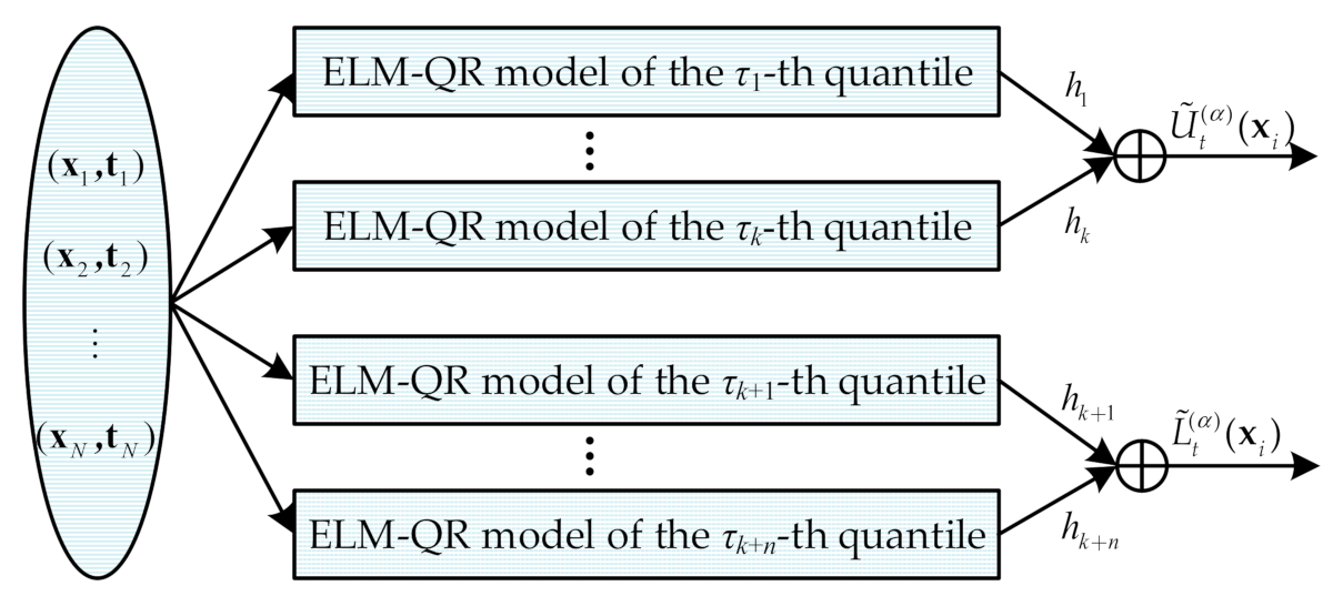
This paper proposes a novel probabilistic prediction model based on the ELM-QR and its structure is shown in Figure 2.
It can be seen from the structure diagram that in order to obtain the lower and upper bounds of the prediction intervals, a certain number of quantile regression models are first trained, and then the outputs of these models are weighted and summed to obtained the corresponding lower and upper bounds of the intervals. In this structure, the quantiles τ 1 τ k , τ 1 > τ 2 > > τ k on which the upper bound depends and the quantiles τ k + 1 τ k + n , τ k + 1 > τ k + 2 > > τ k + n on which the lower bound depends do not cross, and τ k > τ k + 1 .

3.2.2. Solution of the Probabilistic Prediction Model

In the novel probabilistic prediction model, selection of the weighting coefficients will directly affect the range of the prediction intervals, so the setting of the weighting coefficients will be an important part of the probabilistic prediction processes.
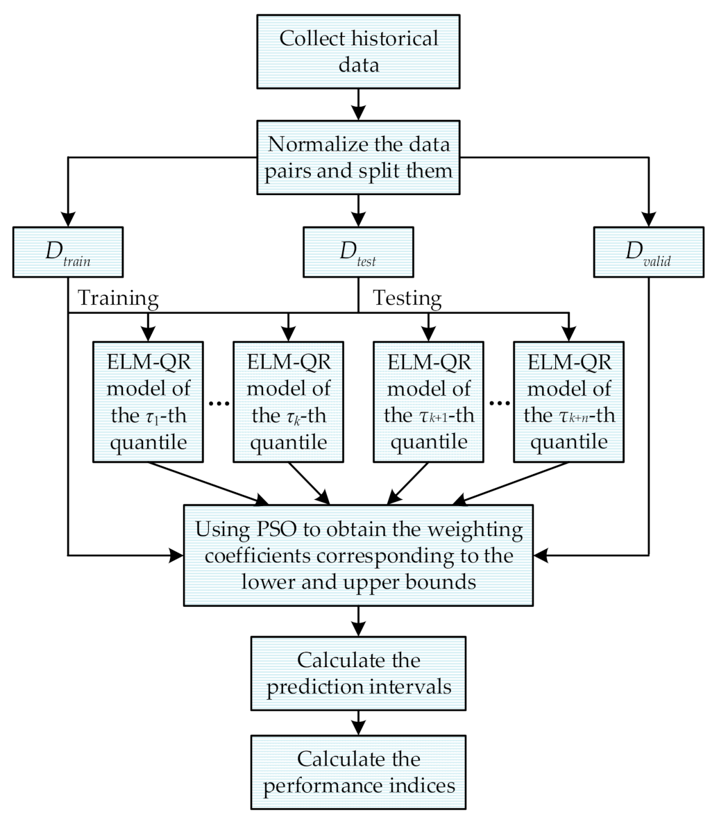
PSO is widely used in various optimization scenarios for its simplicity, superior robustness, and fast convergence speed. In this paper, PSO algorithm is used to obtain the optimal weighting coefficients by maximizing NCI. In order to avoid overfitting, this paper divides the dataset into three categories: D t r a i n , D v a l i d , and D t e s t . Among them, D t r a i n is used to construct the ELM-QR model, D v a l i d and D t r a i n are introduced jointly to optimize the weighting coefficients to enhance generalization ability and avoid overfitting, and D t e s t is used to verify the effectiveness of the algorithm finally.
The calculation process of the wind power probabilistic prediction model based on ELM-QR is shown in Figure 3.
The solution steps are as follows:
Step 1: Collect the actual data of the wind farm, remove dead pixels, construct the input and output data pairs, and normalize the data pairs to [−1,1], divide them into three parts, D t r a i n , D v a l i d and D t e s t ;
Step 2: Set the number of quantile points and the corresponding quantile values, use D t r a i n with the interior point method to obtain the quantile regression models;
Step 3: Initialize the weighting coefficient h t , set γ and λ in the objective function, and initialize the PSO parameters (population number, maximum iteration number, initial velocity and initial position);
Step 4: Use the PSO algorithm to optimize and obtain the weighting coefficients based on D t r a i n and D v a l i d ;
While the maximum number of iterations or sufficiently good fitness has not been reached, perform the following:
(a)
For each particle in the population, calculate the corresponding PI and NCI over Dtrain and Dvalid, NCI is used as the fitness.
(b)
Compare the fitness of particle’s current position with its historical best position (pbest), and update the historical best position with the current position if the fitness of current position is higher.
(c)
Compare the fitness of particle’s current position with the fitness of global best position (gbest). If the fitness of the current position is higher, the global best position is updated with the current position.
(d)
Update particle position and rate according to pbest and gbest.
(e)
Increment the iteration counter.
Step 5: Substitute the inputs of D t e s t into each quantile model to obtain the corresponding outputs, and then determine the prediction intervals according to the weighting coefficients obtained from PSO, and calculate the evaluation indices finally.

4. Case Study

4.1. Simulation Data and Parameter Setting

The actual operating data used in this article is from a wind farm in Hebei province, North China, which covers the period from July to August in 2018 and 2019 with a 15 min sampling period. The wind farm has a combined generating capacity 200.1 MW consisting of 87 wind turbines of 2.3 MW. The wind speed is measured by 70-m-high wind tower and the wind power data is collected by supervisory control and data acquisition (SCADA) system.
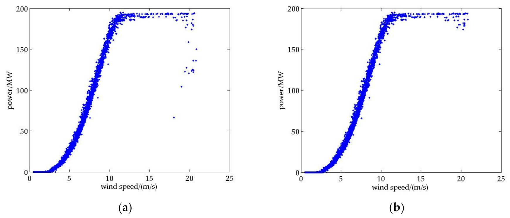
Generally, there are some abnormal data points in the raw data due to sensor failure or communication interruption in daily operation of wind farm. Thus, data processing is required after data collection to ensure high data quality. The data processing method used in this paper is to remove bad points and replace them with liner interpolation data. The raw data and processed data which covers the period from July to August in 2018 is shown in Figure 4, where x-axis is average wind speed measured by wind towers and y-axis is the power of the entire wind farm. It can be seen from Figure 4 that there is a strong mapping relationship between wind speed and power. In [18], the historical wind speed and the historical wind farm power are used as inputs of probabilistic prediction model. However, when the multi-step prediction is performed, the cumulative error will occur because the model input contains the wind farm power (which cannot be obtained from the weather forecast). Therefore, this paper only uses historical wind speed (data covers 8 sampling periods before current time) as input and wind farm power (data at the next sampling period) as output to construct the data pairs for one-step ahead forecasting, and normalizes them to [−1,1]. The subsequent simulations are all based on historical operation data to verify the effectiveness of proposed method. Since the model input is wind speed, which can be easily obtained by weather forecast, so the proposed model is easy to be extended to multi-step prediction through weather forecast data in practical application.
This article mainly tests the prediction results at the nominal confidence level 90% and 80%. For PINC = 90%, set the upper bounds dependent quantiles as 0.90–0.99, and the lower bounds dependent quantiles as 0.01–0.10. For PINC = 80%, the upper bounds dependent quantiles range is chosen as 0.85–0.95, and the lower bounds dependent quantiles range is chosen as 0.05–0.15. The change interval is chosen as 0.01.
D t r a i n contains 4000 sets of data, using data from July to August 2018; D v a l i d contains 480 sets of data from July to August 2019 to increase the generalization ability; D t e s t includes 960 sets of data in 2019.

4.2. Prediction Results

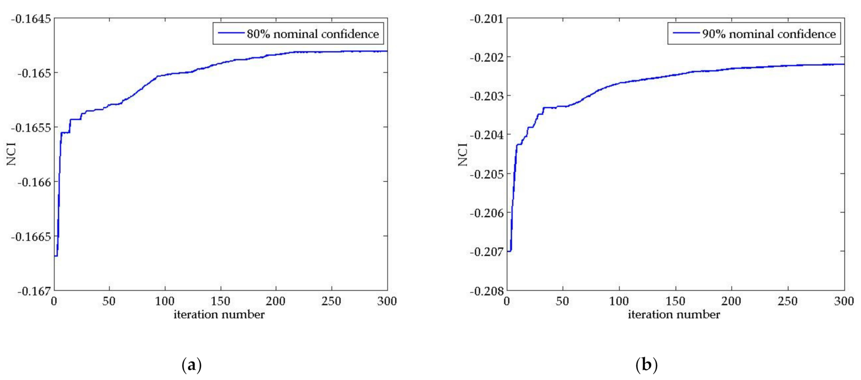
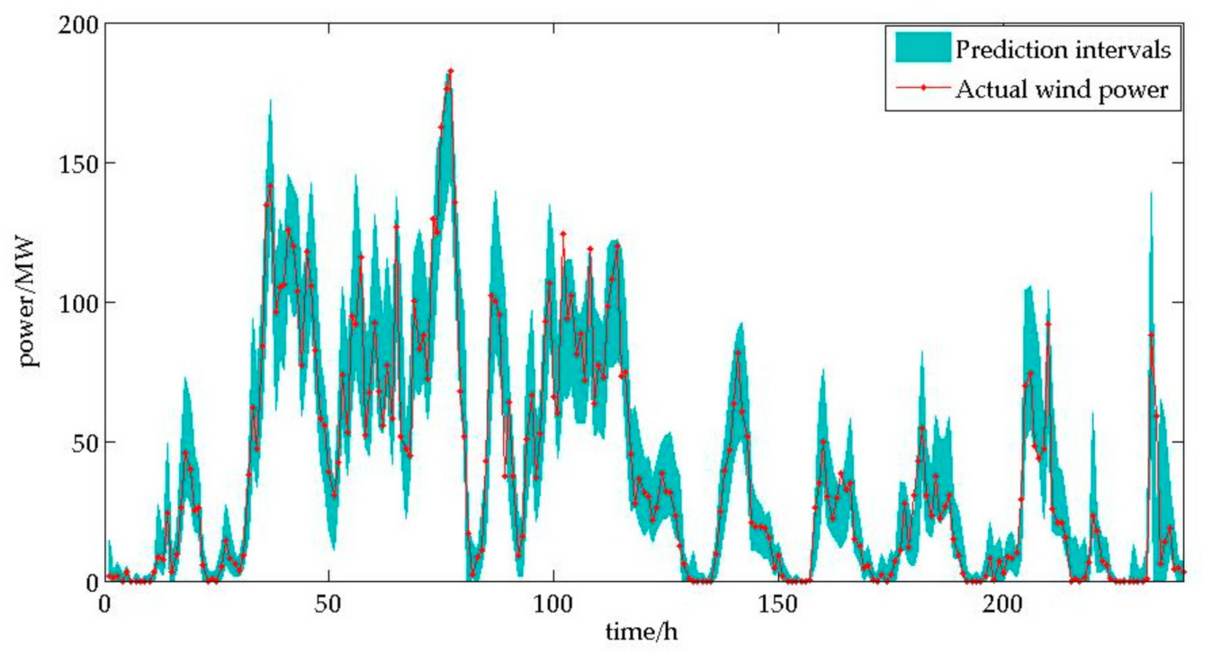
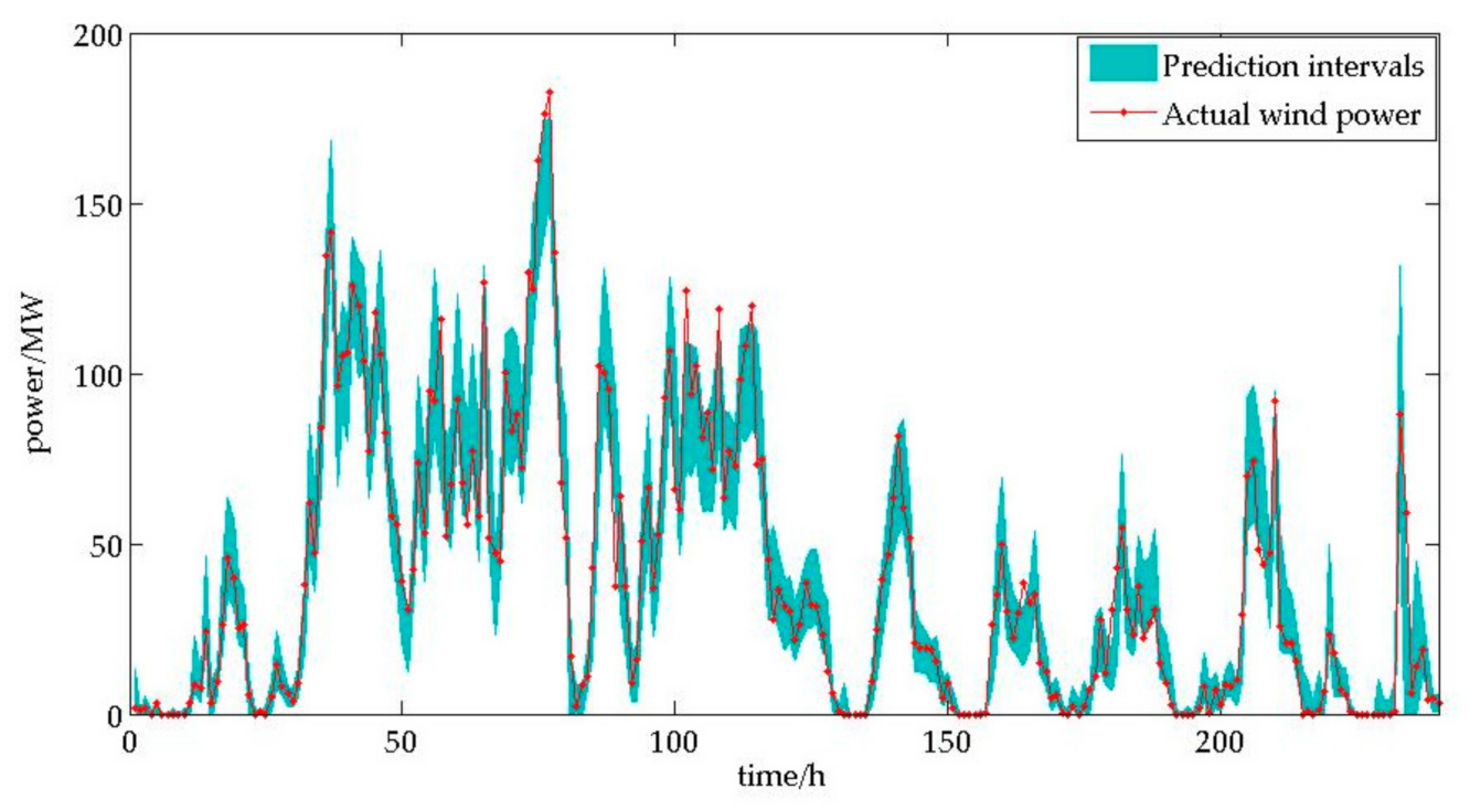
Figure 5 shows the value of NCI with different iteration numbers over training data which is optimized by PSO. With the increases of iteration number, the value of NCI tends to be optimal. Figure 6 and Figure 7 show the prediction results of the test data with PINC = 90% and PINC = 80%, respectively, and Table 1 shows calculation results of the detailed performance indices. It can be seen intuitively from the results in these figures that the obtained prediction intervals are narrow, and the points falling outside the intervals are also close to the interval boundaries. The detailed performance indices calculation results show that the ACE is quite close to 0, and the scores of the interval score and the NCI are also high, which fully shows that the proposed algorithm can obtain a more effective prediction interval.

4.3. Comparative Analysis

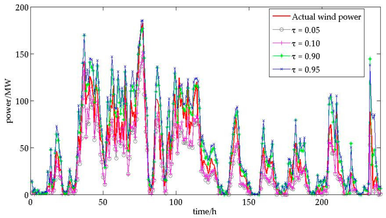
Since in the proposed novel probabilistic prediction model, the lower and upper bounds are obtained by weighted sum of different quantile regression models, in order to further prove the superiorities of this structure, this paper conducts sensitivity analysis on the quantile regression model prediction results, obtain the performance indices of the prediction intervals and compare with the results of the proposed structure. Figure 8 shows the prediction results of some typical quantiles.
The sensitivity coefficient κ is introduced, and its calculation formula is shown in Equation (23), where τ ¯ ,   τ _ are the quantile points corresponding to the upper and lower bounds of the intervals. Calculate various performance indices under different sensitivities and make subsequent comparisons:
τ ¯ τ _ = 1 α κ = 1 τ ¯ τ _
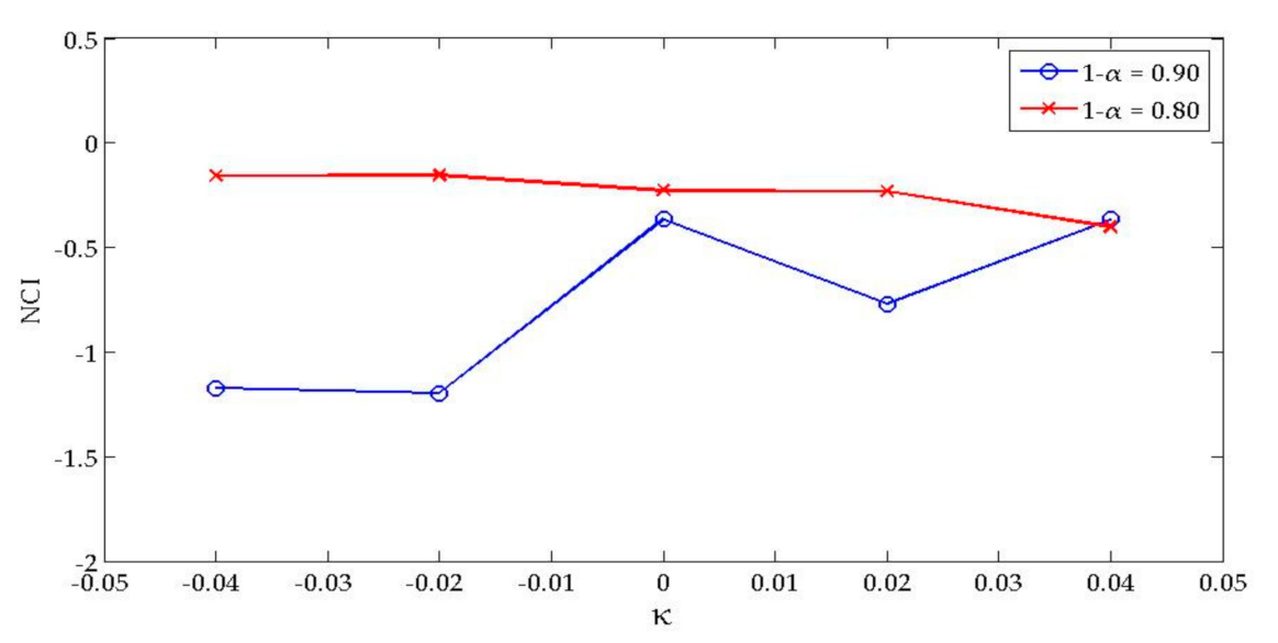
Figure 9 and Table 2 show the NCI results and the detailed performance indices under different sensitivities respectively. From the calculation results, it can be seen that the NCI of the proposed structure is better than the NCI at any sensitivity. With 90% nominal confidence, the ACE and interval scores of the proposed structure are the best; and with 80% nominal confidence, the ACEs with −0.04 and −0.02 sensitivity are better than the proposed structure, but the corresponding interval scores are lower. Considering both of these two situations, the final NCI of the proposed structure is still higher.
Table 3 shows the calculation results of other typical algorithms. Among them, BELM is the algorithm combining bootstrap and ELM in [11], and KDE is the prediction interval obtained by non-parametric kernel density estimation of the prediction errors and combined with the point prediction results. Since KDE depends on the accuracy of point prediction and estimations of the distribution of prediction errors are usually not accurate, so the prediction results are not stable enough. According to the results in Table 3, the ACE of KDE with 90% nominal confidence is high, but the ACE with 80% nominal confidence is low, and they all have a wide prediction interval. For BELM, it assumes that the final result satisfies normal distribution, but this assumption of prior distribution is also not reasonable. At 90% nominal confidence, the result is not as good as that of KDE with almost the same width of prediction interval, but at 80% nominal confidence, the overall result is better than KDE. Combining the calculation results in Table 1, it can be seen that the algorithm proposed in this paper is superior to the above two algorithms in all indicators, which can obtain narrower prediction intervals while ensuring high reliability. The model proposed in this paper can overcome the shortcomings of the above two algorithms, which can get rid of the impact of unreasonable assumptions of prior distribution, and achieve more reasonable and effective prediction intervals based on NCI optimization.

5. Conclusions

In order to obtain effective wind power probabilistic prediction results, this paper proposes a novel type of nonparametric probabilistic prediction method based on ELM-QR. Its main features include:
(1)
Make full use of the fast learning and strong generalization ability of ELM to obtain the quantile regression models effectively.
(2)
A novel comprehensive performance evaluation index is proposed, which can adjust the assessment keypoints adaptively according to different situations, so as to balance reliability and sharpness more reasonably.
(3)
A new model structure is proposed. Based on NCI, the weighting coefficients are obtained through PSO, which fully integrates the advantages of multiple algorithms.
Simulation research and comparative analysis are carried out using actual wind farm operating data. The results show that compared with typical probabilistic prediction methods, the proposed method in this paper can provide more accurate prediction intervals, its comprehensive performance has remarkable advantages, and it can provide effective data support for the safe and stable operation of the power grid.

Author Contributions

Conceptualization: H.N. and Y.L.; methodology: H.N. and Y.L.; software: H.N. and Y.Y.; validation: H.N. and Y.Y.; formal analysis: L.Z.; investigation: H.N.; resources: Y.L.; data curation: H.N.; writing—original draft preparation: H.N. and L.Z.; editing: L.Z. and Y.Y.; visualization: L.Z. and Y.Y.; supervision: Y.L.; project administration: Y.L.; funding acquisition: H.N. and Y.L. All authors have read and agreed to the published version of the manuscript.

Funding

This research was funded by National Key Research and Development Program of China, grant number 2018YFB1502904 and National Natural Science Foundation of China, grant number 51936003.

Institutional Review Board Statement

Not applicable.

Informed Consent Statement

Not applicable.

Data Availability Statement

Data available on request.

Conflicts of Interest

The authors declare no conflict of interest.

References

  1. Zhou, J.Z.; Liu, H.; Xu, Y.H.; Jiang, W. A Hybrid Framework for Short Term Multi-Step Wind Speed Forecasting Based on Variational Model Decomposition and Convolutional Neural Network. Energies 2018, 11, 2292. [Google Scholar] [CrossRef] [Green Version]
  2. Bokde, N.; Feijoo, A.; Villanueva, D.; Kulat, K. A Novel and Alternative Approach for Direct and Indirect Wind-Power Prediction Methods. Energies 2018, 11, 2923. [Google Scholar] [CrossRef] [Green Version]
  3. Yildiz, C.; Acikgoz, H.; Korkmaz, D.; Budak, U. An improved residual-based convolutional neural network for very short-term wind power forecasting. Energy Convers. Manag. 2021, 228. [Google Scholar] [CrossRef]
  4. Duan, J.; Wang, P.; Ma, W.; Tian, X.; Fang, S.; Cheng, Y.; Chang, Y.; Liu, H. Short-term wind power forecasting using the hybrid model of improved variational mode decomposition and Correntropy Long Short-term memory neural network. Energy 2021, 214. [Google Scholar] [CrossRef]
  5. Kisvari, A.; Lin, Z.; Liu, X. Wind power forecasting—A data-driven method along with gated recurrent neural network. Renew. Energy 2021, 163, 1895–1909. [Google Scholar] [CrossRef]
  6. Lange, M. On the uncertainty of wind power predictions—Analysis of the forecast accuracy and statistical distribution of errors. J. Sol. Energy Eng. Trans. ASME 2005, 127, 177–184. [Google Scholar] [CrossRef]
  7. Bludszuweit, H.; Dominguez-Navarro, J.A.; Llombart, A. Statistical analysis of wind power forecast error. IEEE Trans. Power Syst. 2008, 23, 983–991. [Google Scholar] [CrossRef]
  8. Bruninx, K.; Delarue, E. A Statistical Description of the Error on Wind Power Forecasts for Probabilistic Reserve Sizing. IEEE Trans. Sustain. Energy 2014, 5, 995–1002. [Google Scholar] [CrossRef]
  9. Liu, F.; Pan, Y.; Liu, H.; Ding, Q.; Li, Q.; Wang, Z. Piecewise Exponential Distribution Model of Wind Power Forecasting Error. Autom. Electr. Power Syst. 2013, 37, 14–19. [Google Scholar]
  10. Guan, J.; Lin, J.; Guan, J.; Mokaramian, E. A novel probabilistic short-term wind energy forecasting model based on an improved kernel density estimation. Int. J. Hydrog. Energy 2020, 45, 23791–23808. [Google Scholar] [CrossRef]
  11. Wan, C.; Xu, Z.; Pinson, P.; Dong, Z.Y.; Wong, K.P. Probabilistic Forecasting of Wind Power Generation Using Extreme Learning Machine. IEEE Trans. Power Syst. 2014, 29, 1033–1044. [Google Scholar] [CrossRef] [Green Version]
  12. Sun, M.; Feng, C.; Zhang, J. Multi-distribution ensemble probabilistic wind power forecasting. Renew. Energy 2020, 148, 135–149. [Google Scholar] [CrossRef]
  13. Wan, C.; Lin, J.; Wang, J.H.; Song, Y.H.; Dong, Z.Y. Direct Quantile Regression for Nonparametric Probabilistic Forecasting of Wind Power Generation. IEEE Trans. Power Syst. 2017, 32, 2767–2778. [Google Scholar] [CrossRef]
  14. Hu, J.M.; Tang, J.W.; Lin, Y.Y. A novel wind power probabilistic forecasting approach based on joint quantile regression and multi-objective optimization. Renew. Energy 2020, 149, 141–164. [Google Scholar] [CrossRef]
  15. Cai, L.; Gu, J.; Ma, J.H.; Jin, Z.J. Probabilistic Wind Power Forecasting Approach via Instance-Based Transfer Learning Embedded Gradient Boosting Decision Trees. Energies 2019, 12, 159. [Google Scholar] [CrossRef] [Green Version]
  16. He, Y.; Li, H.; Wang, S.; Yao, X. Uncertainty analysis of wind power probability density forecasting based on cubic spline interpolation and support vector quantile regression. Neurocomputing 2020. [Google Scholar] [CrossRef]
  17. He, F.; Zhou, J.; Mo, L.; Feng, K.; Liu, G.; He, Z. Day-ahead short-term load probability density forecasting method with a decomposition-based quantile regression forest. Appl. Energy 2020, 262. [Google Scholar] [CrossRef]
  18. Yang, X.; Fu, G.; Zhang, Y.; Kang, N.; Gao, F. A Naive Bayesian Wind Power Interval Prediction Approach Based on Rough Set Attribute Reduction and Weight Optimization. Energies 2017, 10, 1903. [Google Scholar] [CrossRef] [Green Version]
  19. Wan, C.; Xu, Z.; Pinson, P.; Dong, Z.Y.; Wong, K.P. Optimal Prediction Intervals of Wind Power Generation. IEEE Trans. Power Syst. 2014, 29, 1166–1174. [Google Scholar] [CrossRef] [Green Version]
  20. Shrivastava, N.A.; Lohia, K.; Panigrahi, B.K. A multiobjective framework for wind speed prediction interval forecasts. Renew. Energy 2016, 87, 903–910. [Google Scholar] [CrossRef]
  21. Hu, M.Y.; Hu, Z.J.; Yue, J.P.; Zhang, M.L.; Hu, M.Y. A Novel Multi-Objective Optimal Approach for Wind Power Interval Prediction. Energies 2017, 10, 419. [Google Scholar] [CrossRef]
  22. Shrivastava, N.A.; Khosravi, A.; Panigrahi, B.K. Prediction Interval Estimation of Electricity Prices Using PSO-Tuned Support Vector Machines. IEEE Trans. Ind. Inform. 2015, 11, 322–331. [Google Scholar] [CrossRef]
  23. Al-Musaylh, M.S.; Deo, R.C.; Li, Y. Electrical Energy Demand Forecasting Model Development and Evaluation with Maximum Overlap Discrete Wavelet Transform-Online Sequential Extreme Learning Machines Algorithms. Energies 2020, 13, 2307. [Google Scholar] [CrossRef]
  24. Al-Dahidi, S.; Ayadi, O.; Adeeb, J.; Alrbai, M.; Qawasmeh, B.R. Extreme Learning Machines for Solar Photovoltaic Power Predictions. Energies 2018, 11, 2725. [Google Scholar] [CrossRef] [Green Version]
  25. Wang, L.; Li, X.; Bai, Y. Short-term wind speed prediction using an extreme learning machine model with error correction. Energy Convers. Manag. 2018, 162, 239–250. [Google Scholar] [CrossRef]
  26. Luo, J.; Wong, C.-M.; Vong, C.-M. Multinomial Bayesian extreme learning machine for sparse and accurate classification model. Neurocomputing 2021, 423, 24–33. [Google Scholar] [CrossRef]
  27. Peng, X.; Zheng, W.; Zhang, D.; Liu, Y.; Lu, D.; Lin, L. A novel probabilistic wind speed forecasting based on combination of the adaptive ensemble of on-line sequential ORELM (Outlier Robust Extreme Learning Machine) and TVMCF (time-varying mixture copula function). Energy Convers. Manag. 2017, 138, 587–602. [Google Scholar] [CrossRef]
  28. Xiao, L.; Shao, W.; Jin, F.; Wu, Z. A self-adaptive kernel extreme learning machine for short-term wind speed forecasting. Appl. Soft Comput. 2021, 99. [Google Scholar] [CrossRef]
  29. Yang, H.-F.; Chen, Y.-P.P. Representation learning with extreme learning machines and empirical mode decomposition for wind speed forecasting methods. Artif. Intell. 2019, 277. [Google Scholar] [CrossRef]
  30. Zheng, W.; Peng, X.; Lu, D.; Zhang, D.; Liu, Y.; Lin, Z.; Lin, L. Composite quantile regression extreme learning machine with feature selection for short-term wind speed forecasting: A new approach. Energy Convers. Manag. 2017, 151, 737–752. [Google Scholar] [CrossRef]
  31. Ul Haque, A.; Nehrir, M.H.; Mandal, P. A Hybrid Intelligent Model for Deterministic and Quantile Regression Approach for Probabilistic Wind Power Forecasting. IEEE Trans. Power Syst. 2014, 29, 1663–1672. [Google Scholar] [CrossRef]
  32. Huang, G.B.; Zhu, Q.Y.; Siew, C.K. Extreme learning machine: Theory and applications. Neurocomputing 2006, 70, 489–501. [Google Scholar] [CrossRef]
  33. Huang, G.B.; Zhou, H.M.; Ding, X.J.; Zhang, R. Extreme Learning Machine for Regression and Multiclass Classification. IEEE Trans. Syst. Man Cybern. Part B 2012, 42, 513–529. [Google Scholar] [CrossRef] [PubMed] [Green Version]
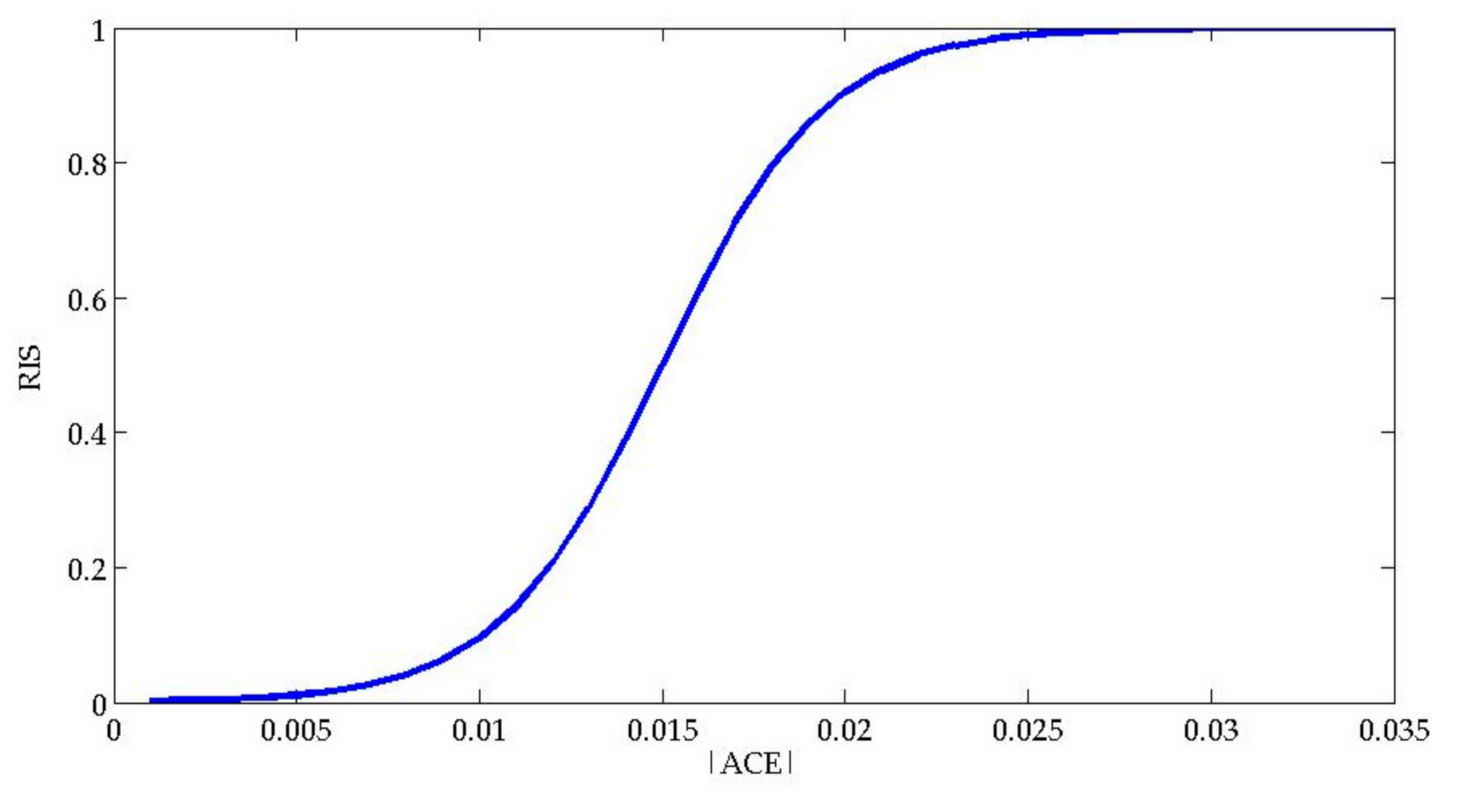
Figure 1. Curve of RIS changing with |ACE|.
Energies 14 00701 g001
Figure 2. Structure of the proposed novel probabilistic prediction model.
Energies 14 00701 g002
Figure 3. Calculation flowchart of the proposed wind power probabilistic prediction model.
Energies 14 00701 g003
Figure 4. Wind speed-power diagram: (a) the raw data; (b) the processed data.
Energies 14 00701 g004
Figure 5. The value of NCI with different iteration numbers over training data: (a) At 80% nominal confidence; (b) at 90% nominal confidence.
Energies 14 00701 g005
Figure 6. Prediction results at the nominal confidence level 90%.
Energies 14 00701 g006
Figure 7. Prediction results at the nominal confidence level 80%.
Energies 14 00701 g007
Figure 8. Prediction results of some typical quantiles.
Energies 14 00701 g008
Figure 9. The NCI results with different sensitivities.
Energies 14 00701 g009
Table 1. Performance indices calculation results.
PINCPICPACEScoreNCI
90%89.17%−0.83%−3.73%−0.234
80%79.69%−0.31%−5.96%−0.154
Table 2. Detailed performance indices under different sensitivities.
PINCκPICPACEScoreNCI
90%−0.0487.71%−2.29%−4.01%−1.173
−0.0286.98%−3.02%−3.97%−1.197
088.85%−1.15%−3.92%−0.365
0.0288.44%−1.56%−3.98%−0.769
0.0488.85%−1.15%−3.92%−0.365
80%−0.0480.10%0.10%−6.20%−0.157
−0.0280.10%0.10%−6.08%−0.155
079.06%−0.94%−6.14%−0.227
0.0279.06%−0.94%−6.27%−0.230
0.0478.75%−1.25%−6.25%−0.401
Table 3. Detailed performance indices of different algorithms.
PINCMethodsPICPACEScoreNCI
90%BELM88.02%−1.98%−4.74%−1.133
KDE91.52%1.52%−4.76%−0.807
80%BELM79.79%−0.21%−7.33%−0.186
KDE78.96%−1.04%−7.28%−0.295
Publisher’s Note: MDPI stays neutral with regard to jurisdictional claims in published maps and institutional affiliations.