Application of Decision Trees for Optimal Allocation of Harmonic Filters in Medium-Voltage Networks

Abstract

The paper proposes a solution for the problem of optimizing medium voltage power systems which supply, among others, nonlinear loads. It is focused on decision tree (DT) application for the sizing and allocation of active power filters (APFs), which are the most effective means of power quality improvement. Propositions of some DT strategies followed by the results have been described in the paper. On the basis of an example of a medium-voltage network, an analysis of the selection of the number and allocation of active power filters was carried out in terms of minimizing losses and costs keeping under control voltage total harmonic distortion (THD) coefficients in the network nodes. The presented example shows that decision trees allow for the selection of the optimal solution, depending on assumed limitations, expected effects, and costs.

1. Introduction

These days, when we observe rapid technological progress and constantly increasing energy consumption, it is necessary to pay attention to responsible energy utilization. Electrical energy supply, especially in highly developed regions, is achieved through energy transmission. The concept of alternating current (AC) power systems, which was assumed many years ago, makes the monitoring of some power quality indices below limits necessary. It is more and more challenging as the number of loads having a negative influence on these indices increases. The distortion of voltage and current waveforms, which is caused by nonlinear loads and manifests itself through higher harmonics, belongs to the most important power quality parameters, and it is expressed by the total harmonic distortion (THD) coefficient. The higher harmonic elimination and, thereby, THD minimization is a basic task given to power quality improvement systems.

The placement of compensation devices, including active power filters (APFs), in power networks is one of the key factors in successful power quality improvement not only from the technical but also from the economical point of view. In many cases, filters have to be applied in complex and large power networks with several nonlinear loads and a significant number of nodes. Among these nodes there are numerous ones to which APFs or other devices ensuring high power quality can be connected. Thus, a system designer has to be able to solve an optimization problem that consists in location of the devices ensuring, among others, effective higher harmonic elimination while keeping the solution costs under control.

The optimization of passive and active power filter parameters and location in power systems is a common problem among researchers all over the world due to its crucial role in the attainment of power quality goals. There are many propositions of solutions based on diverse optimization methods that implement classical algorithms or try to develop problem specific ones. The proposed solutions differ in complexity, universality, and most of all the degree to which practical aspects of implementation of power quality systems have been taken into account. The simplest approach to filter location is just the iterative examination of power quality improvement obtained when installing it in successive nodes one by one [1]. The best solution is chosen by comparison of the results. Such an approach can be extended to more sophisticated forms based on the adaptive step presented recently in [2]. The proposed algorithm uses a decision tree and achieves an excellent harmonic suppression effect for an exemplary circuit using less number and capacity of APFs when compared with a solution calculated by a traditional method [2]. This paper also follows this direction in the research aimed at optimal APF location and sizing. In the past, many approaches have been proposed for solution of the problem under consideration. The advanced solutions have been based on complex optimization algorithms, e.g., ant colony system [3], modified harmony search algorithm [4], whale optimization algorithm [5], gray wolf optimizer [6], and bacterial foraging optimization algorithm [7]. Nevertheless, the most popular approaches are based on genetic algorithms [8,9,10,11] and particle swarm optimization [12,13,14].

Among optimization goals, one can find a minimization of the power losses [15,16,17], which has been used also in this paper along with an economic criterion expressed by the relative cost of the solution. The distinctive feature of this paper is minimization of the power losses caused by the higher harmonics in all system elements (mainly electric cables and transformers). Such an approach is especially efficient in relatively small networks working with little power margin and, thus, exposed to overloads or replacements of main and expensive components, e.g., transformers. The size of the network encouraged us to check the performance of decision trees as a tool for APF location and sizing. So far, decision trees in the field of power systems have been applied to:

• optimal phasor measurement unit (PMU) placement for voltage security assessment [18,19], including power system islanding identification [20] and line outage detection [21,22,23]—fast and direct measurement results by PMUs combined with decision trees gives more time for corrective or preventive actions;
• classification and detection of power line faults [24,25,26];
• detection of power system problems, including power quality disturbances [27], active power imbalance [28], voltage stability margin [29], and nontechnical losses [30,31];
• fault location in power distribution systems [32,33,34];
• optimal planning of storage in power systems integrated with wind power generation [35];
• decision-making in single-device cases [36] as well as in global power plant operation [37].

Thus, decision trees are widely used in power systems—they belong to the 10 major machine learning models frequently used in power systems [38]. However, literature overview has revealed no evidence regarding the application of decision trees to solve the problem under consideration, i.e., APF location. The only similar research includes application of decision trees for the determination of optimal location and rate of series compensation to increase power system loading margin [39]. The paper [39] is focused on series compensation of transmission lines, which is one of the most effective means to increase the loading margin of an interconnected power system. It includes a proposition of methodology for the identification of the critical transmission lines and their proper compensation rate with respect to voltage stability using decision trees. It must be stressed that the application of decision trees in various areas resulted in several descendant methods, for example, random forest [40] and gradient boosted trees [41]. The random forest, as a technique consisting in the aggregation of a large number of decision trees, is usually regarded as a black-box algorithm due to the large number of trees. Gradient-boosted trees represent another approach, which belongs to the so called “ensemble methods” based on more than one decision tree. Such methods are especially useful in solving large-scale problems. They have also been applied in power systems, for example, in the building load model [42]. In this paper, due to the scale of the problem and its type, which is optimization rather than classification or prediction, a classical form of the decision tree algorithm was used.

In this paper, the authors proposed decision trees as an algorithm to solve the problem of APF location in medium voltage networks. For a given test system and two goal functions, the results have been compared with the global optimum obtained by the brute force algorithm. The paper consists of three sections with an introduction. Section 2 is devoted to APF optimum sizing and location, and it includes the definitions of goal functions as well as the description of the brute force and decision tree algorithms. Section 3 includes the description of the test system and optimization results for brute force and decision tree algorithms. Section 4 and Section 5 present the result discussion and conclusions.

2. Optimization Problem Definitions and Solution Algorithms

2.1. Goal Functions

This paper proposes optimization of APF placement in power systems based on two different goal functions. The general denotation, R_k, has been introduced in order to formalize goal function descriptions, where R_k is k-th element of a set of all possible APF configurations. It specifies the placement of each APF in the discussed power system in relation to the list of all APFs denoted by K.

$$R_k=\left[s_1 s_2 \cdots s_i\right],$$

(1)

where

• $s_i$—state of the APF in i-th node (1—APF placed, 0—no APF),
• for all APF list $K=\left[n_1 n_2 \cdots n_i\right]$, where $n_i$—denotation of i-th APF.

Along with the goal functions, all optimization processes take into account the maximum value of voltage total harmonic distortion coefficient (THDV) factor occurring in the system. A maximum allowed THDV level of 5% has been assumed for all optimization methods presented in this paper.

2.1.1. Power Losses Criterion

The first implemented goal function is related to criterion of active power losses in system elements:

$$\underset{x}{\min }{F}_1\left(x\right): \underset{R_k}{\min }{\displaystyle \sum }_{m=1}^M{P}_m,$$

(2)

where

• $m$—number of power system elements in which power losses occur (transformers, lines, coils, etc.), $m=1, 2, \dots , M$.
• $P_m$—power losses of m-th element.
• $x$—independent variable of the goal function that is subjected to minimization.

The minimization of F₁ function allows reduction of power losses related not only with harmonics but also with reactive power in all system elements excluding loads. Due to the fact that even with full compensation, loads require power transfer, F₁ cannot be reduced completely to 0.

2.1.2. Cost Criterion

Application of the dispersed power quality improvement system is related with the necessity of considering many possible solutions that rely on the placement of at least several APFs. For such an approach, economic criterion is of high importance. A fundamental factor influencing the costs of a solution consists of a set of rated parameters of used APFs and results from conditions imposed by the power system. On the grounds of market recon, public information provided by APF producers and literature overview, a nonlinear function of APF price has been presented below. It was scaled in order to indicate price relative to the most expensive APF. The bar graph of APF relative cost depending on the range of rated current has been shown in Figure 1.

The cost criterion has been described formally through F₂ goal function, formulated as follows:

$$\underset{x}{\min }{F}_2\left(x\right):\underset{R_k}{\min }{\displaystyle \sum }_{i=1}^{N}p\left(\left|I_i^k\right|\right),$$

(3)

where

• $p\left(·\right)$—function assigning the cost to i-th APF depending on its RMS current value,
• $i$—APF number, $i=1, 2, \dots , N$,
• $\left|I_i^k\right|$—RMS current of i-th APF, calculated as:

$$\left|I_i^k\right|=\sqrt{{\displaystyle \sum }_{h=1}^H{\left|I_{ih}^k\right|}^2},$$

(4)

where

• $\left|I_{ih}^k\right|$—RMS current of h-th harmonic of i-th APF,
• $h$—harmonic number, $h=1, 2, \dots , H$.

2.2. Brute Force Algorithm

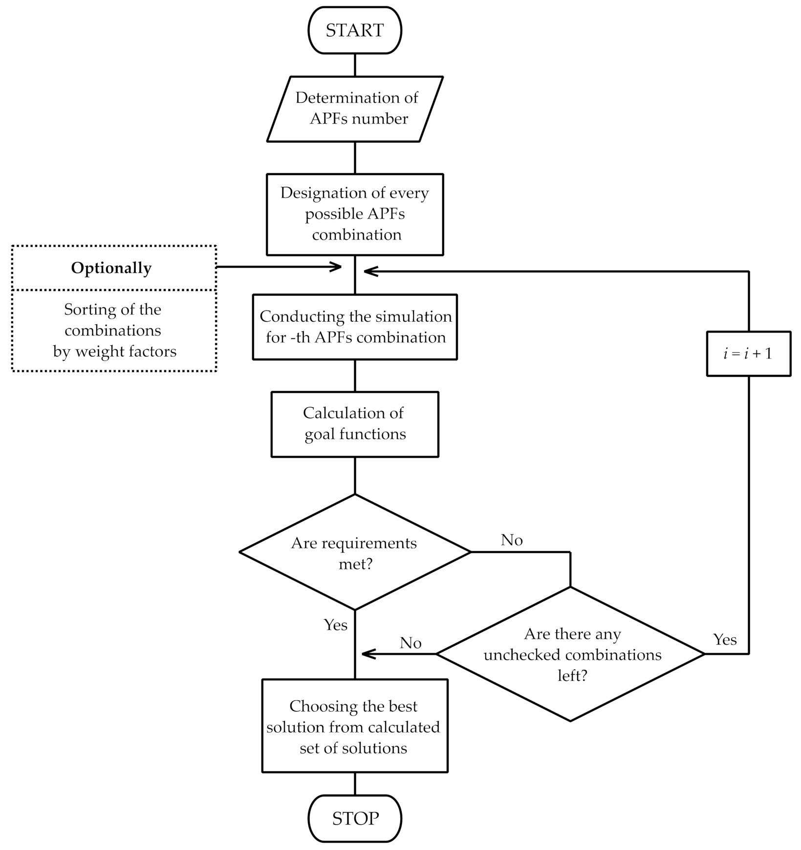
The problem of APF sizing and allocation has been solved using a brute force (BF) algorithm, which due to computation times is especially useful in the case of small-scale problems. In this paper, the BF algorithm allows us to find all solutions, including the global minimum, and evaluate the quality of solutions obtained by the decision tree (DT) algorithm. The block diagram of the BF algorithm has been presented in Figure 2.

The BF algorithm is very straightforward and consists in checking every combination representing in our case different allocations of APFs in the power system. If the power system has n nodes (the number of nodes in which APFs can be connected, not the total number of nodes), the number of k-combinations is equal to the binomial coefficient:

$$C_n^k=\left(\begin{array}{c}n\\ k\end{array}\right)=\frac{n!}{k!\left(n-k\right)!}.$$

(5)

In successive steps of the BF algorithm, values of the given goal function (2) or (3) are calculated. The algorithm can be terminated before analyzing all combinations if the goal function value drops below the assumed threshold value—in this case there is no guarantee that the global minimum has been reached. Otherwise, it is terminated if all combinations have been checked. Afterward, the best solution is chosen.

2.3. Optimization with Decision Trees

The application of decision trees is the most popular in classification problems in which an algorithm uses a set of features that can be checked one by one. Such a method is efficient and allows the effective solving of similar issues. However, classification problems are not the only one class of problems that can be addressed with decision trees, and this method can be also applied in general combinatorial optimization. This paper proposes a solution for the application of decision trees in the optimization of APF placement in power systems. Such an issue can be formulated as the problem of deciding where APFs should be placed in order to get the best possible results in terms of previously defined goal functions.

An implemented decision tree algorithm works iteratively by checking which step should be taken next in order to reduce the current value of the minimized goal function. The APF combination through which the algorithm passes is coded in a vector representing the state of each APF (1).

The algorithm operation begins with a state in which only one APF is placed in the power system, on a previously defined starting position. In the next steps, the algorithm makes a decision whether the current APF should be moved to the next or the previous node from R_k vector or whether it should remain in the current position and another one should be placed additionally. There is also a possibility to terminate the decision tree’s operation if any of the aforementioned options does not provide a better outcome. The criterion of the decision-making process can be formulated through the difference between the current value of the goal function and a value that could be reached by each possible decision:

$$\min \left(∆f_{+}, ∆f_{-}, ∆f_{add}, ∆f_0\right)$$

(6)

where

• $∆f_{+}$—difference between goal function values for the current state and a state after moving the APF to the next node,
• $∆f_{-}$—difference between goal function values for the current state and a state after moving the APF to the previous node,
• $∆f_{add}$—difference between goal function values for the current state and a state after adding a new APF, modified by the correctional coefficient, W_corr,
• $∆f_0$—zero value connected with staying in the current state.

In order to keep the balance between the advantages and disadvantages of adding a new APF, the decision tree algorithm was also fitted with a correctional coefficient, W_corr, which allows the regulation of how many times benefits from adding a new APF should be higher than benefits from moving it in order to make such a decision. With appropriate configuration, this coefficient prevents a cost increase, which would occur due to the tendency for adding new APFs in each step while reducing power losses.

The schematic of the recurring element of the decision tree has been presented in Figure 3. The components of this diagram can only be modified in border cases related to reaching the maximum allowed number of APFs, or the lack of movement possibilities—in all other cases, the structure repeats itself until the termination of the algorithm. Such conditions, limiting decision tree’s options, include also the THDV value. The whole optimization process is related to improving power quality quantities such as THDV along with the minimized function. In order to guarantee such improvement, only solutions that result in a THDV value below 5% can be accepted. The decision tree can only terminate its action if the THDV is below this level, otherwise it continues its search.

3. Optimization Results

3.1. Test System

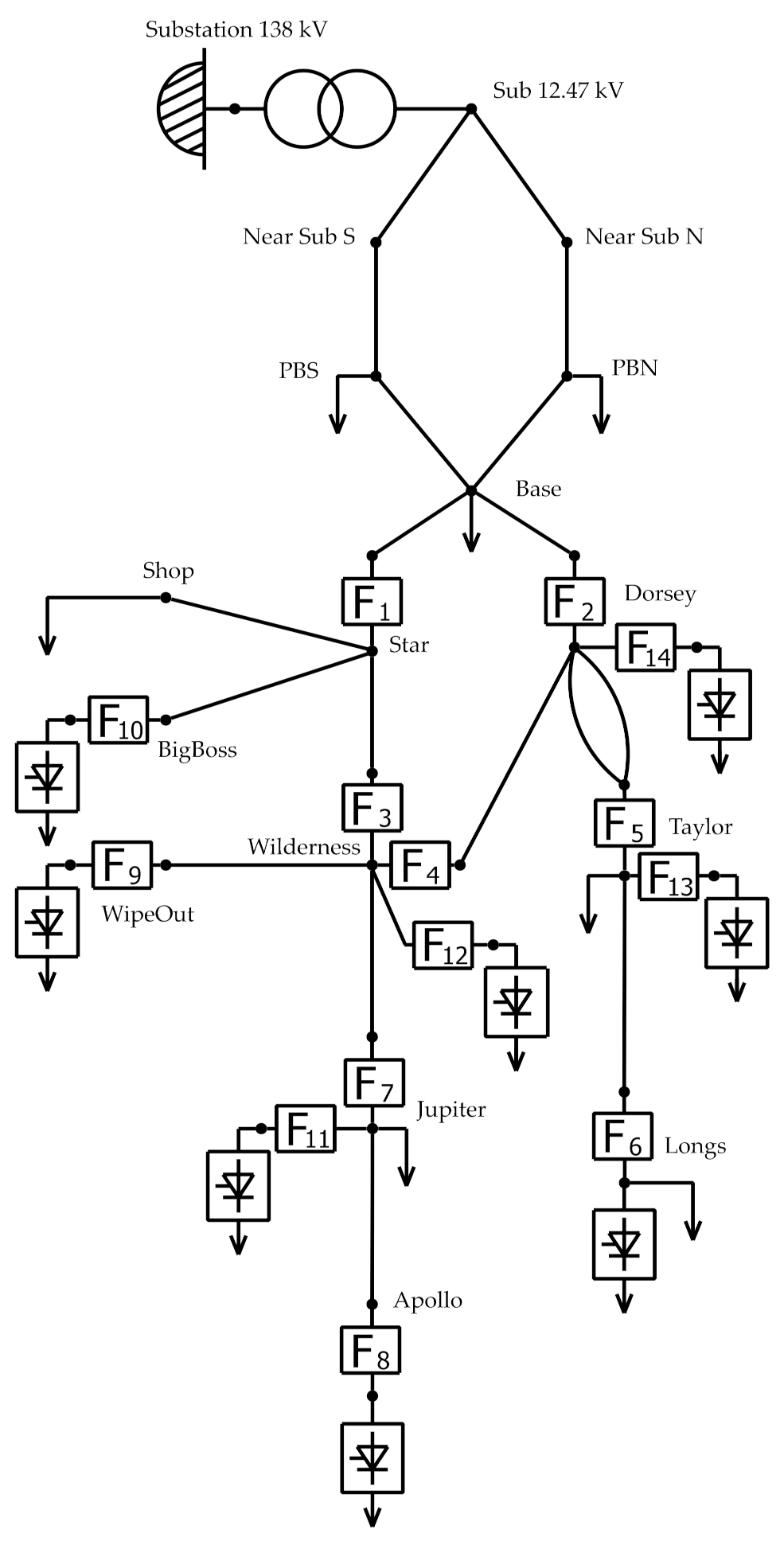
In this paper, a test system was adopted based on the power supply scheme of an extended ski station. The data on the system and its topology have been taken from the documentation of the PCFLO simulation software [43] and are often used in other papers [9,44,45]. The advantages of the selected test system are its complexity, the presence of nonlinear loads, access to complete information on its components, and medium voltage for which there are technical solutions of APF systems. The diagram of the system with marked potential connection points of active power filters is presented in Figure 4.

It should be noted that despite the series connection of APFs (F₁–F₁₄) in the test power system, the APF itself is constructed as parallel, based on a current-controlled current source (Figure 5). The nonlinear loads in the presented system are six pulse rectifiers, which are the cause of current and voltage waveform distortions in the entire circuit. The modeling and simulation software based on the iterative method in the frequency domain described in [46] was used for calculations. In this case, a simple, without losses, ideal model of the active power filter was used in the simulations (Figure 5).

Table 1. Values of voltage total harmonic distortion coefficients (THDVs) for all voltage nodes and current total harmonic distortion coefficients (THDIs) for all line currents.

Node Name	Node Number	THDV, %	Line	THDI, %
Sub 12.47 kV	1	11.3	20-1	11.0
Near Sub S	2	11.4	1-2	11.0
Near Sub N	3	11.4	1-3	11.0
PBS	4	11.7	2-4	10.9
PBN	5	11.7	3-5	10.9
Base	6	11.9	4-6	12.2
Star	7	12.4	5-6	12.2
Wilderness	8	12.5	6-7	22.3
Dorsey	9	12.4	6-9	19.3
Taylor	10	12.4	7-16	3.4
Longs	11	12.5	7-15	30.7
Apollo	12	13.1	7-8	16.7
Jupiter	13	12.8	8-9	40.2
WipeOut	14	12.7	8-14	32.8
BigBoss	15	13.0	8-13	23.0
Shop	16	12.4	13-12	29.7
Sub 138 kV	20	3.3	9-10	6.9
			10-11	6.1

summarizes the voltage total harmonic distortion coefficients (THDVs) for all nodes and the current total harmonic distortion coefficients (THDIs) for all lines of the analyzed system in the case without APFs.

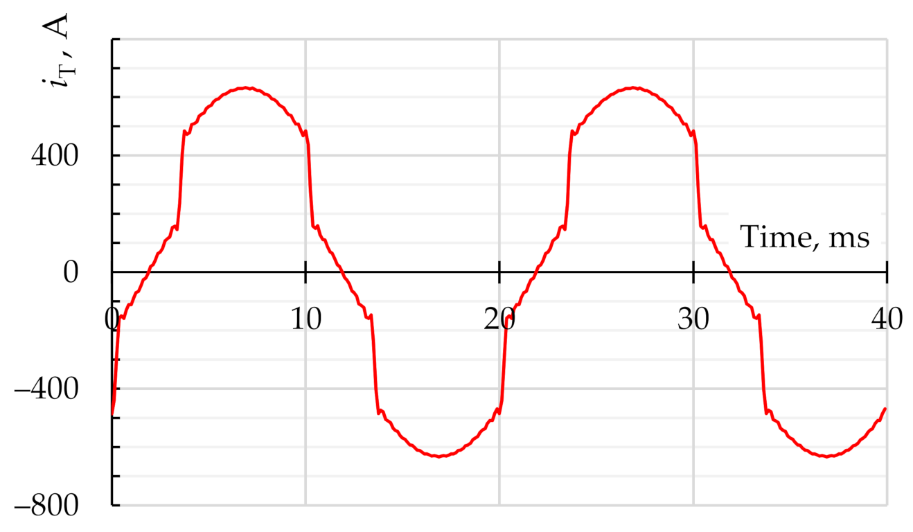
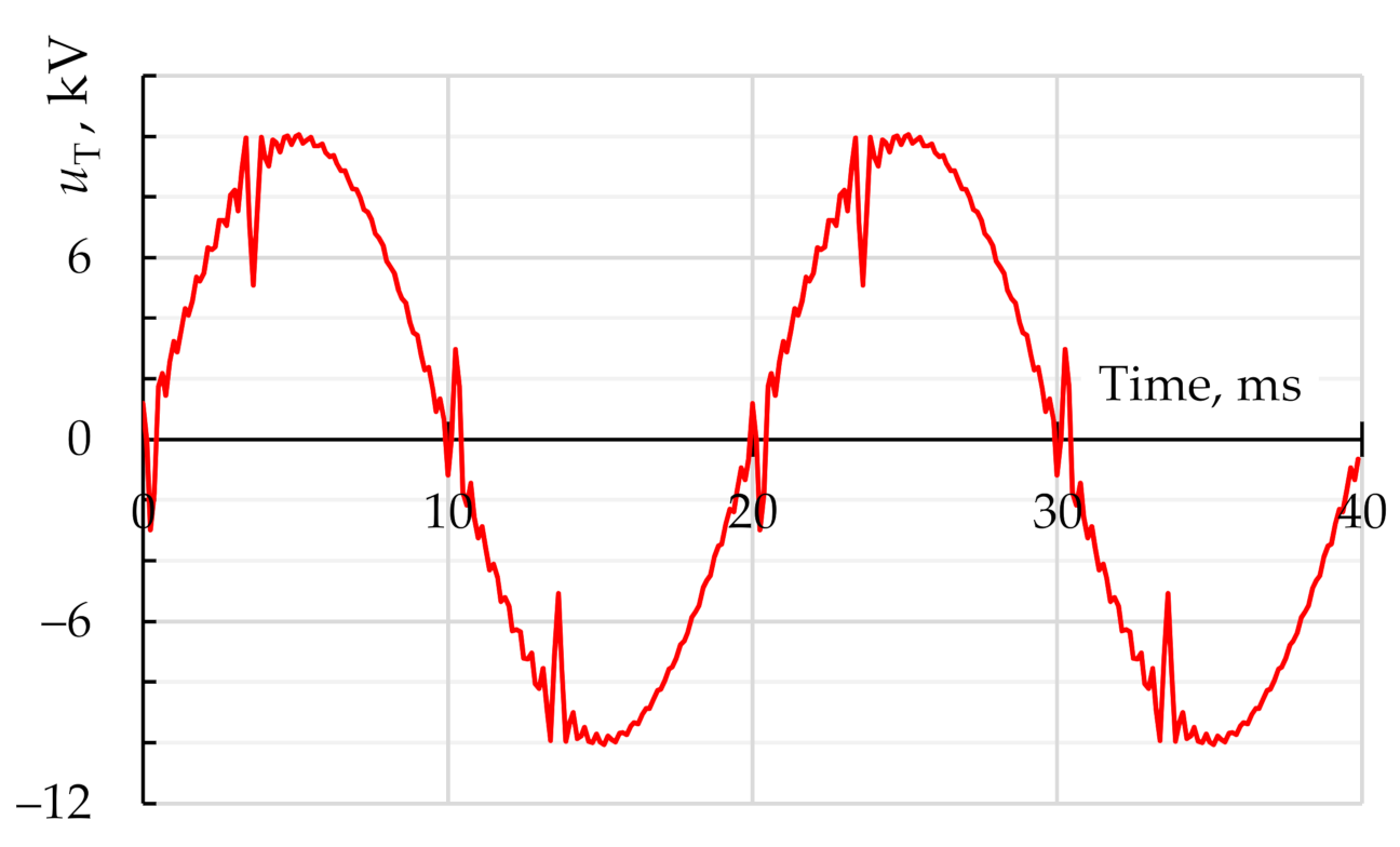
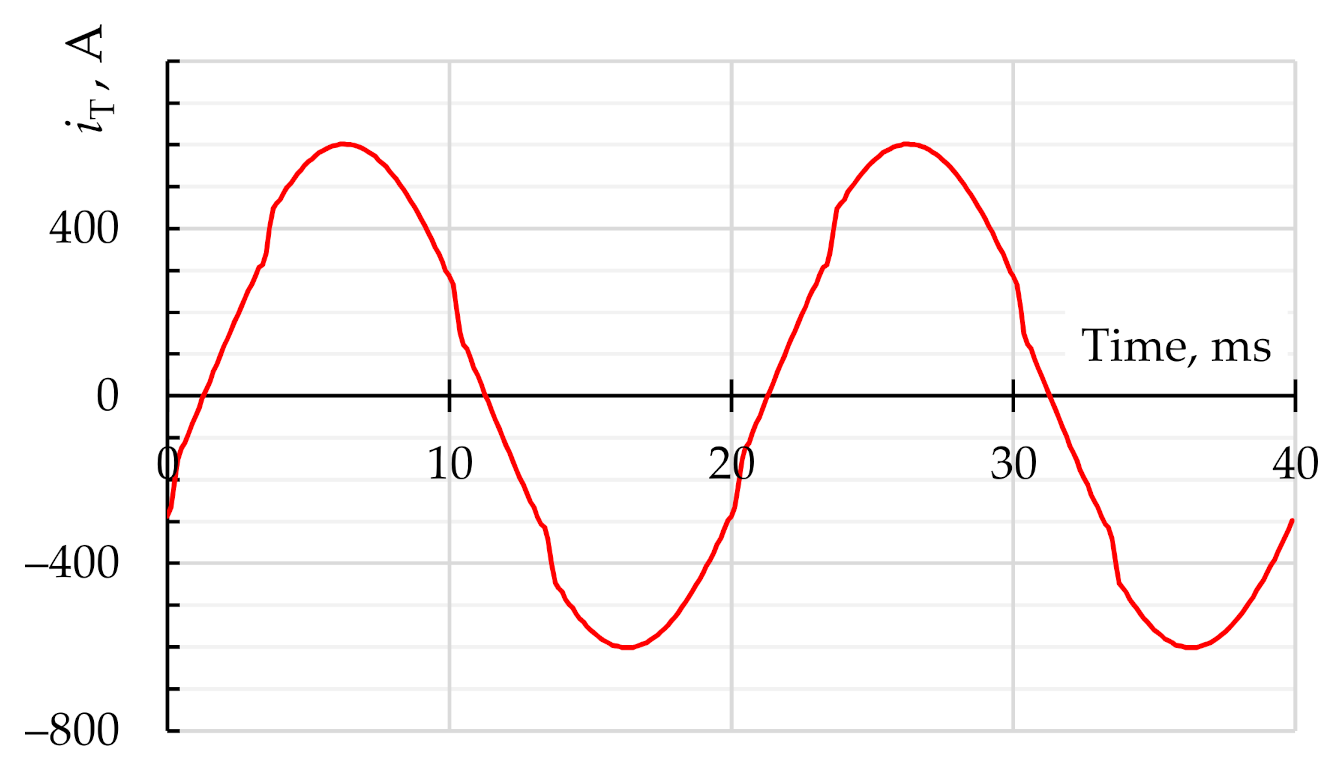
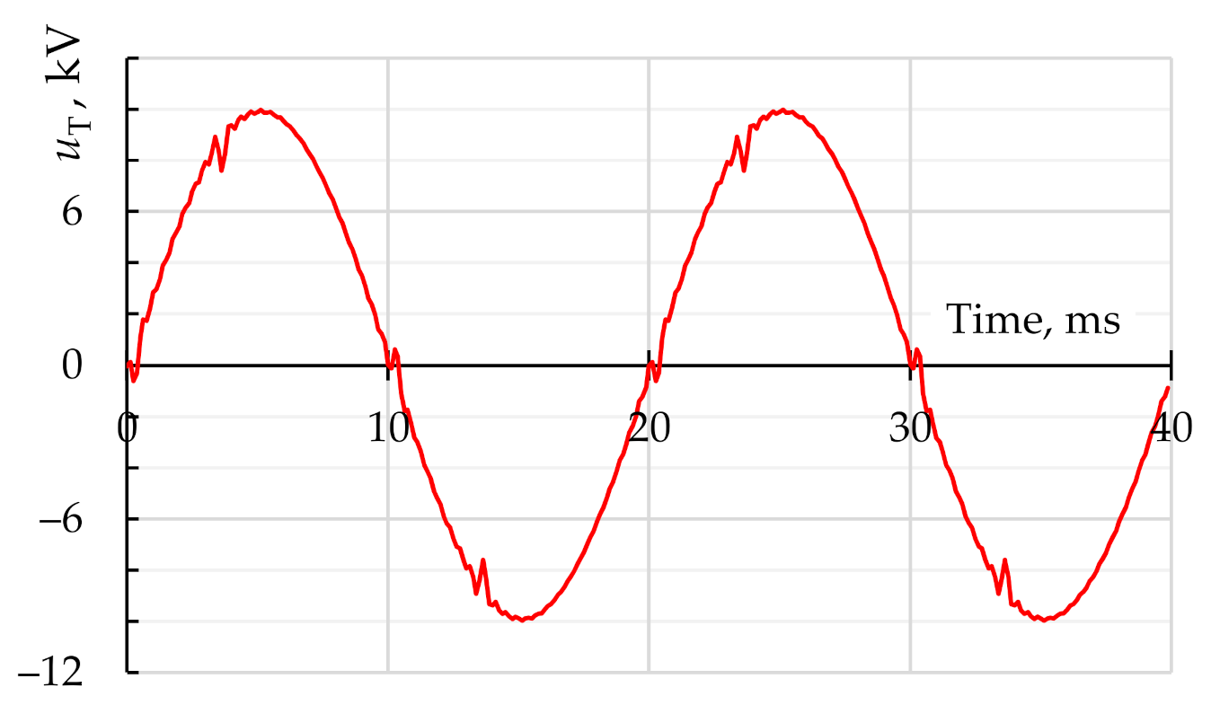
As can be seen in Table 1, the THDV and THDI values are significant and can potentially cause power losses and power quality problems in the analyzed system. Distortion is also visible in the transformer current and voltage waveforms, which have been shown in Figure 6 and Figure 7, respectively. The voltage waveform shows instantaneous voltage drops, which increase the THD coefficient. These drops are due to the high steepness of the transformer output current. The oscillations around these drops result directly from the used model of nonlinear receivers and the simulation method in the frequency domain. The presented waveforms are a combination of a finite number of harmonics obtained as a result of simulations and not measured waveforms.

3.2. Brute Force Results

As a part of the work, optimization by means of the brute force method was carried out in order to compare results with those of the proposed method based on decision trees. The obtained results have been analyzed and presented below. The first aspect related to the operation of the algorithm is the calculation time, which in the case of the complete solution set search method may be long enough to prevent the efficient use of the software. Along with the increase in the number of possible cases according to Equation (5), the time needed to analyze all the combinations increased. Figure 8 presents both the aforementioned quantities as a function of the number of APFs, the arrangement of which was optimized. The obtained results confirm that such an approach, when applied to complex problems, despite its high effectiveness, may not be the optimal choice.

Table 2. List of cases meeting the minimum criterion of the analyzed goal functions, taking into account the assumed maximum of THDVs.

APF Numbers	Number of APFs
	For a Minimum of F1
1	2
2	3	10
3	2	8	10
4	3	5	8	10
5	2	6	8	10	11
6	2	3	4	8	10	13
7	1	2	4	6	8	10	11
	For a Minimum of F2
1	1
2	4	10
3	4	10	13
4	4	8	10	12
5	4	8	9	10	14
6	2	3	4	8	10	13
7	4	7	8	9	10	12	13

contains the APF connection cases, which were selected by the software as the best in terms of minimizing each of the considered goal functions with the limitation related to the maximum THDV coefficient. From these data, it can be seen that the best solutions for a small number of APFs are in most cases the solutions for a larger number of APFs.

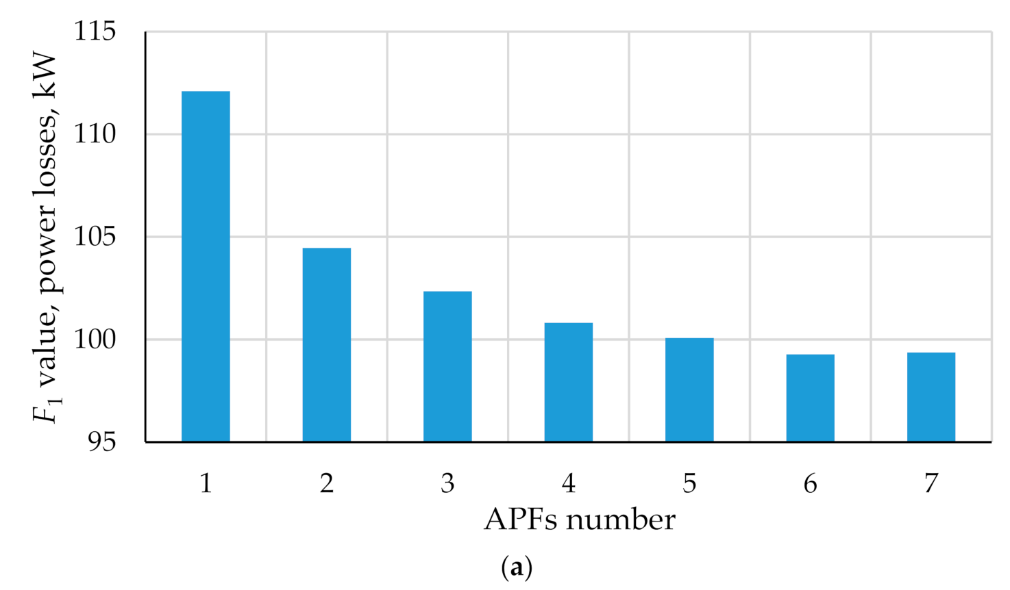
The impact of placing subsequent APFs on the values achieved by the individual goal functions in the cases selected as optimal was also analyzed. The results were presented for the group with the limitation resulting from the maximum allowable THDV level. The results of this analysis have been shown in Figure 9. For the goal function F₁, the increase in the number of APFs results in a clear decrease in power losses, which is natural and results directly from the concept of an APF, i.e., harmonic reduction and reactive power compensation. In the case of the goal function F₂, the relative value (related to the maximum APF cost) was used. With the assumption of limiting the THDV factor, the minimum costs for the case with two APFs is visible. Reaching the required maximum THDV in the system is, therefore, the most cost effective when using two APFs. Any other solution is more expensive.

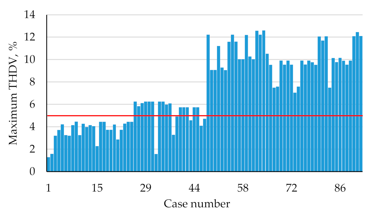
All the results obtained by applying the brute force algorithm, even before the analysis in terms of finding the minimum for the individual goal functions, are in the form of a set of values of these functions associated with each possible solution. For a larger number of APFs, the number of cases is so large that the graphical representation becomes unclear, therefore an example bar graph of the maximum THDV value in the system for selecting the position of only two APFs has been presented below (Figure 10). This graph shows how large the variability of the maximum THDV is for the analyzed cases.

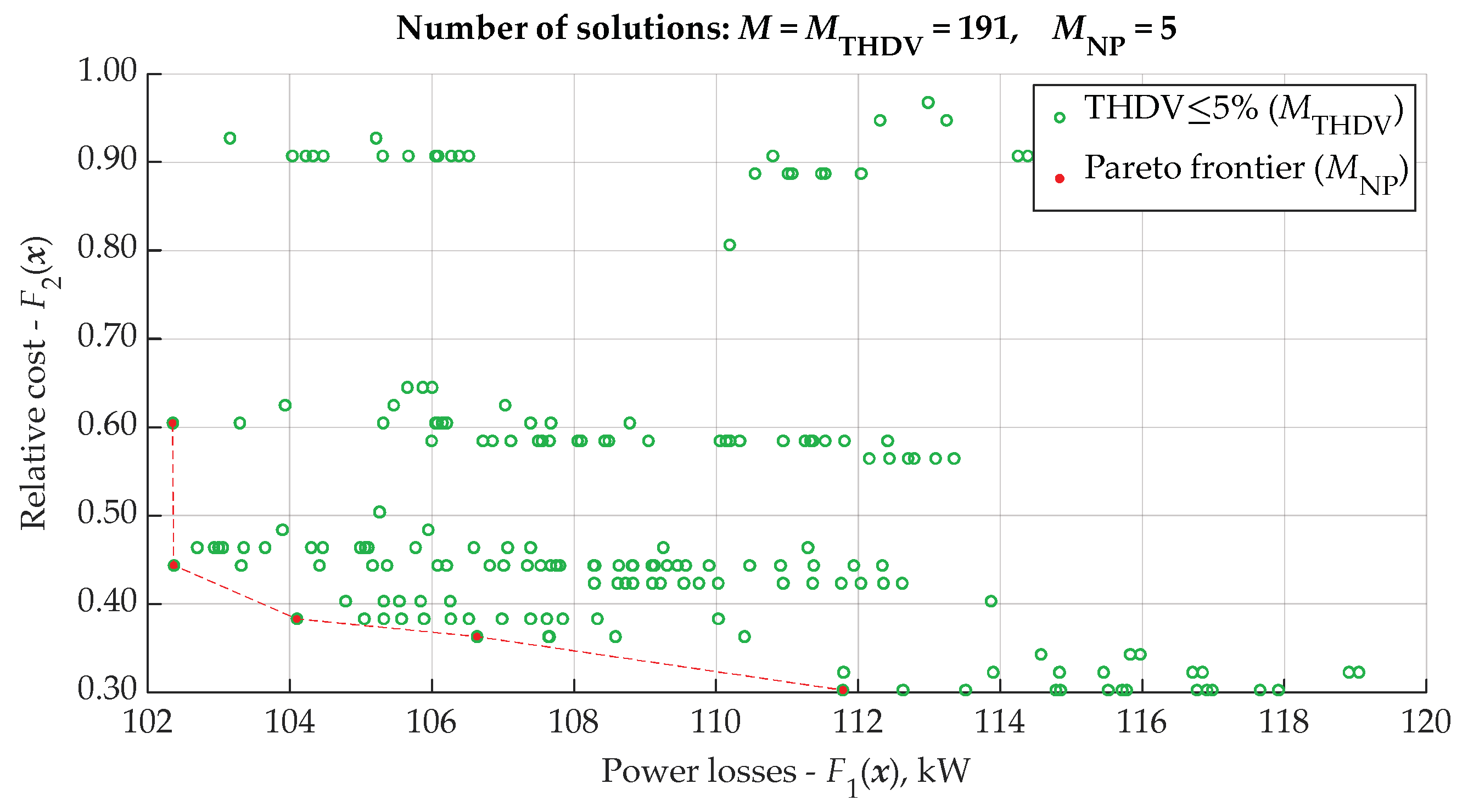
In order to illustrate the results from a wider perspective, for the case of three APFs in the system, all feasible solutions have been presented in Figure 11. As can be read, for 191 solutions out of 364 (see Figure 8) the constraint on the THDV coefficient (less or equal 5%) is fulfilled. Moreover, the Pareto frontier includes five solutions for which the objective functions given by (2) and (3) take approximately the values between 102 and 112 kW for F₁ and between 0.30 and 0.60 for F₂. These solutions are optimal in the Pareto sense and the choice of the one to be implemented depends on other aspects, e.g., easier APF allocation in some nodes or long-term financial analysis. Therefore, selection of the optimum solution can vary among decision-makers because it is based on their preferences and criteria.

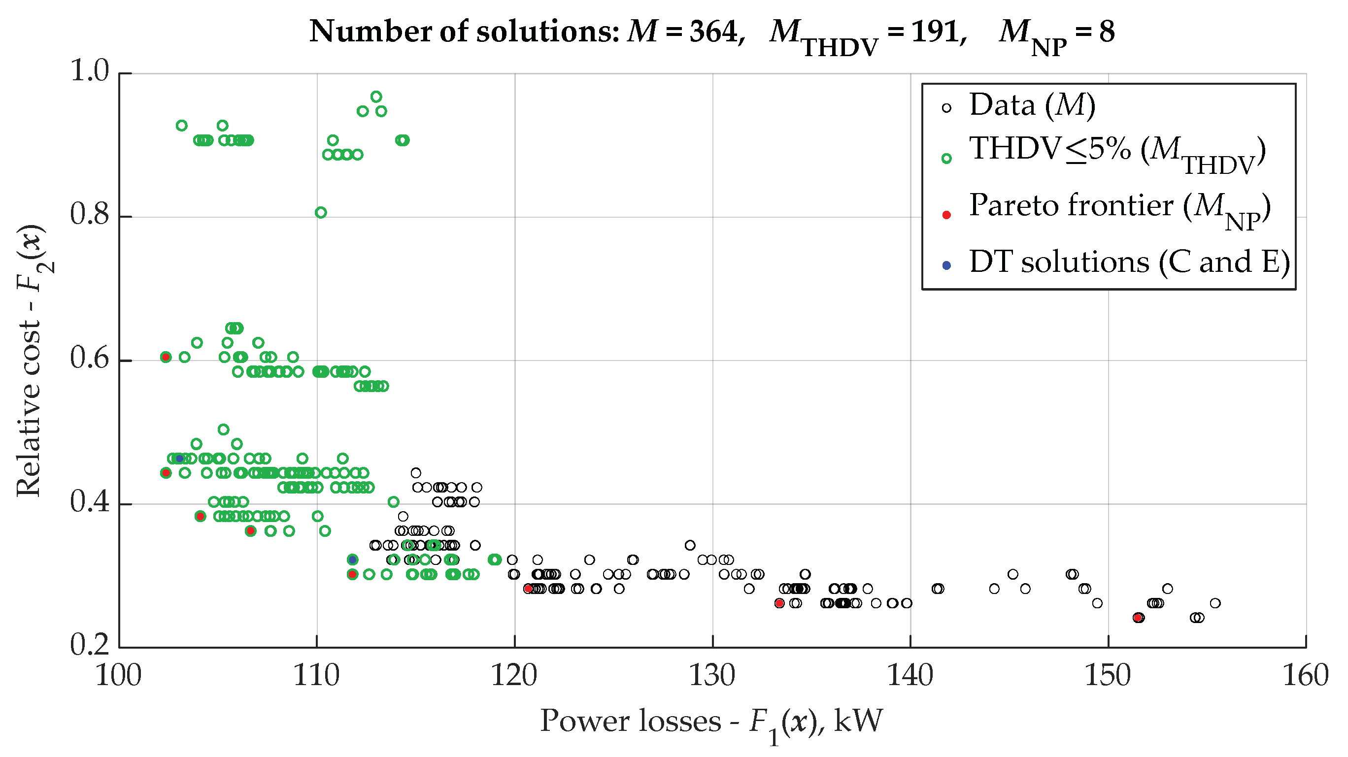
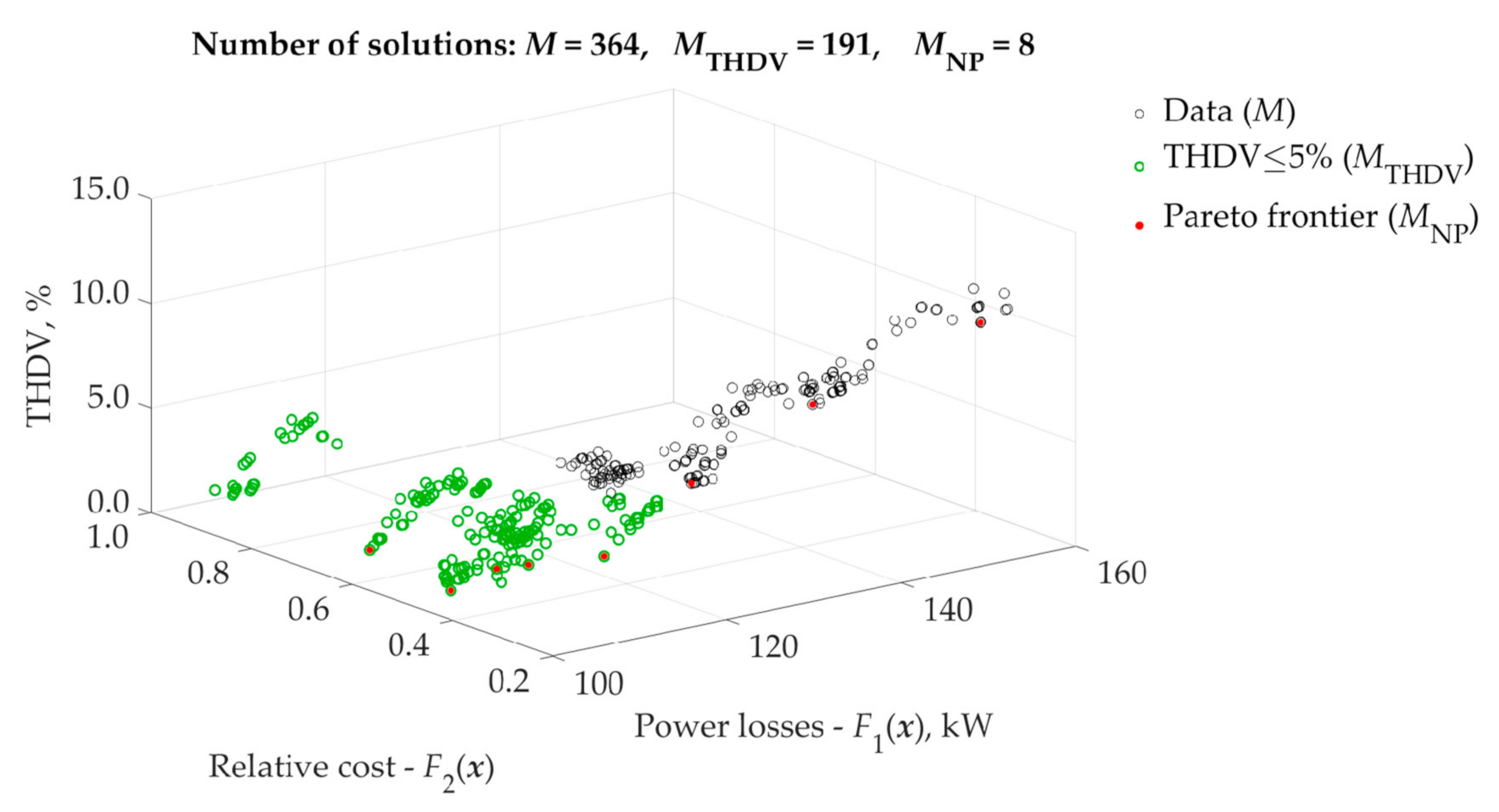
All solutions for three APFs presented in Figure 12 allow us to have a deeper insight into this example. The Pareto frontier in such a case consists of eight points representing the optimum solutions for the unconstrained problem. The feasible points presented in Figure 11, for which THDV ≤ 5%, have been also marked out in Figure 12. The same data have been presented in 3D space in Figure 13.

3.3. Decision Tree Results

Optimization with the decision tree algorithm is challenging considering how complex the hierarchical structure of the power system is. The first factor affecting the decision-making process is the algorithm’s starting point. The decision tree is highly sensitive to the choice of the starting point because it determines the position of the first APFs that are going to be checked. Consequently, different parts of the simulated power system can be examined at the beginning. The mentioned problem is only a specific case of the more general issue of arrangement of APF combination in a single solution vector, R_k. In a particular case, it only results in the change of the starting point. Considering the high importance of APF arrangement, and therefore the algorithm’s route, different strategies of its setup have been examined. The optimization has been conducted for both F₁ and F₂ goal functions with differences between routes that arise from different methods of sorting the APFs in R_k vector. The research assumes three sorting strategies: by node THDV value (descending), by APF current value (ascending), and by APF number (descending). Another factor differentiating tested routes is the W_corr coefficient, which has been included and excluded in turns, for the consecutive algorithm workflows. The results for all tested approaches have been presented in

Table 3. List of route parameters and results of the decision tree algorithm applied for F₁ and F₂ minimization.

Index	Minimized Function	Route Sorted by	Wcorr	F1, kW	F2	Calculation Time, s	APF Number	Number of Installed APFs
A	F1	THDV	Yes	111.8	0.32	1.4	3	10, 7, 11
B	F1	THDV	No	100.4	0.69	1.3	7	8, 10, 7, 11, 9, 6, 3
C	F1	Number of APF	Yes	103.0	0.46	1.4	3	10, 7, 3
D	F1	Number of APF	No	99.4	1.23	4.3	14	14, 13, 12, 11, 10, 9, 8, 7, 6, 5, 4, 3, 2, 1
E	F2	THDV	Both	111.8	0.32	0.7	3	10, 7, 11
F	F2	Number of APF	Both	105.6	0.54	2.1	6	13, 12, 11, 10, 9, 8
G	F1	Current	Yes	108.7	0.40	1.3	4	13, 10, 11, 7
H	F1	Current	No	99.4	1.15	3.9	13	12, 14, 9, 13, 6, 8, 10, 11, 7, 5, 4, 1, 2
I	F2	Current	Both	110.1	0.54	2.2	6	14, 9, 13, 6, 8, 10

.

As presented, different routes result in a different number of placed APFs and optimization efficiency. The application of this method highly reduces computation time in comparison to the brute force algorithm. The calculation time mostly depends on the number of steps taken by the decision tree, because in each step, before the decision, the algorithm repeats simulation the same number of times. The only exceptions occur if the algorithm encounters a position where the number of possible choices is limited, and in that case, there is no need for repeating the simulation for every option.

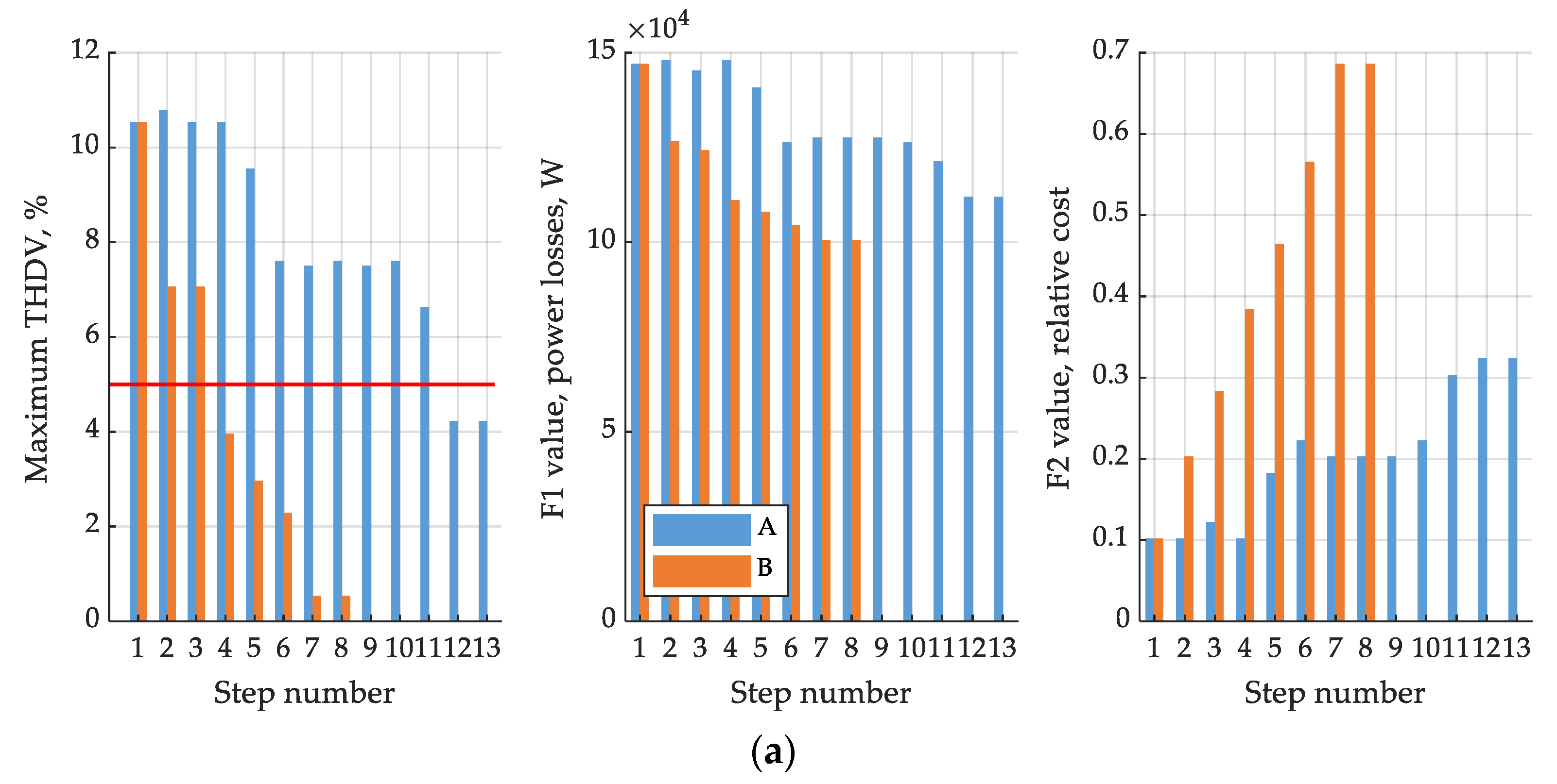
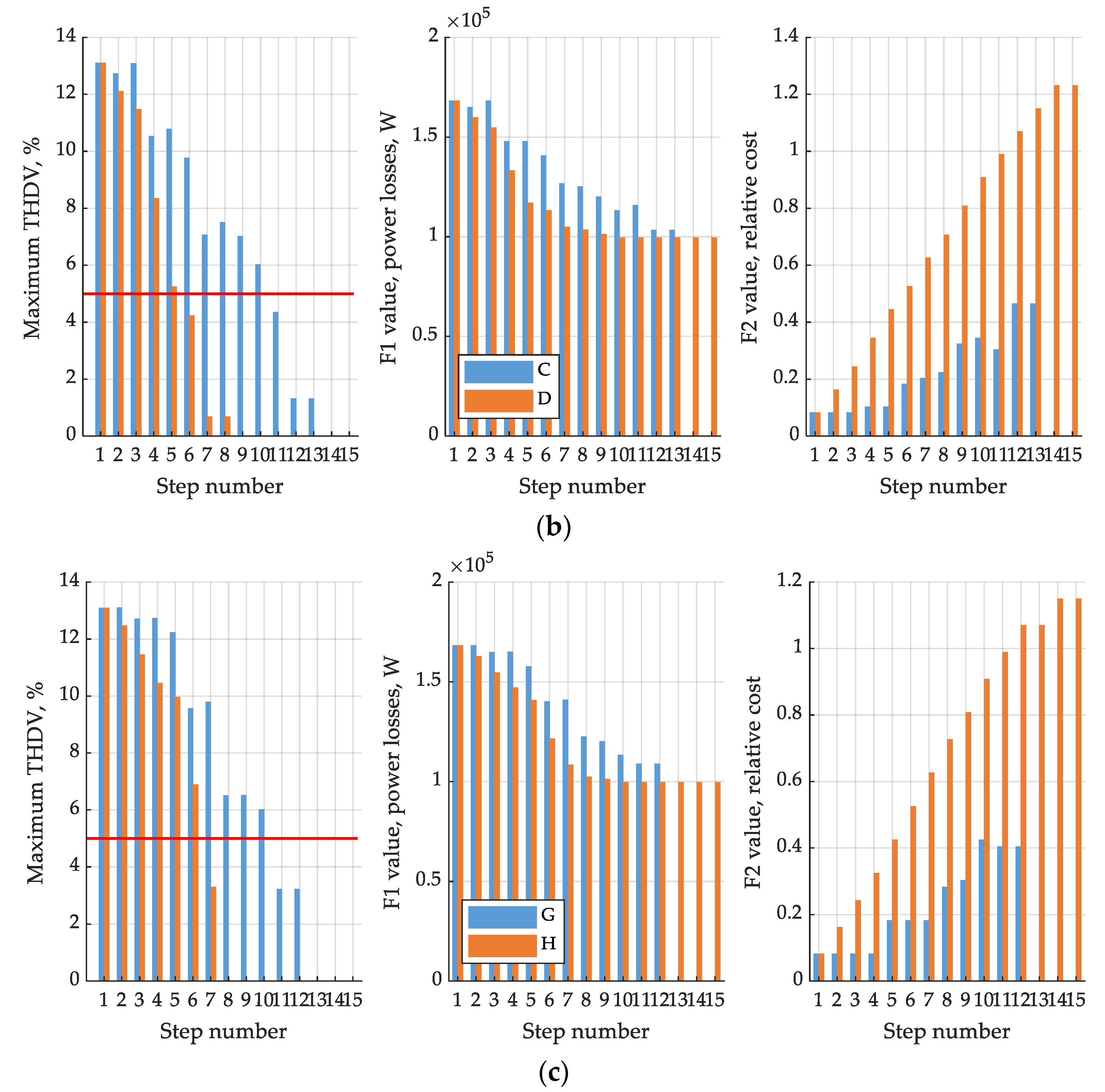
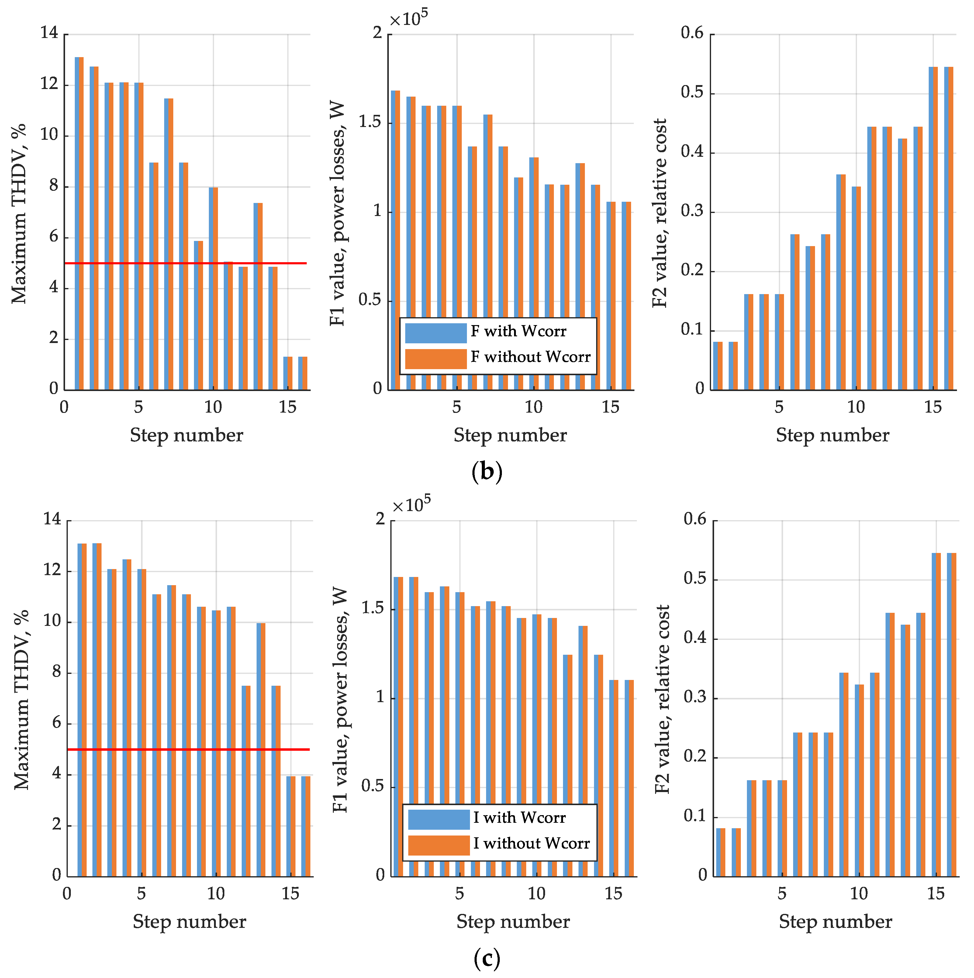
Figure 14 and Figure 15 present THDV, F₁, and F₂ values for each step of the decision tree algorithm. Results were grouped in such a way that each axis contains a representation of routes differing from each other only by presence of the W_corr coefficient. Figure 14 shows routes for F₁ minimization and Figure 15 for F₂ minimization. In the case of F₁, every solution shows a clear tendency of reducing power losses in the system for each step taken. This effect is connected with placing additional APFs or with moving APFs to better positions. The requirement of reducing the THDV coefficient below 5% level enforces placing more than one APF, which consequently raises the cost of the solution. It is worth stressing that the THDV limitation requirement also causes the algorithm to increase the cost of the solution by placing another APF even during F₂ minimization. The reduction of costs can only be achieved and is visible in cases when the THDV requirements are met.

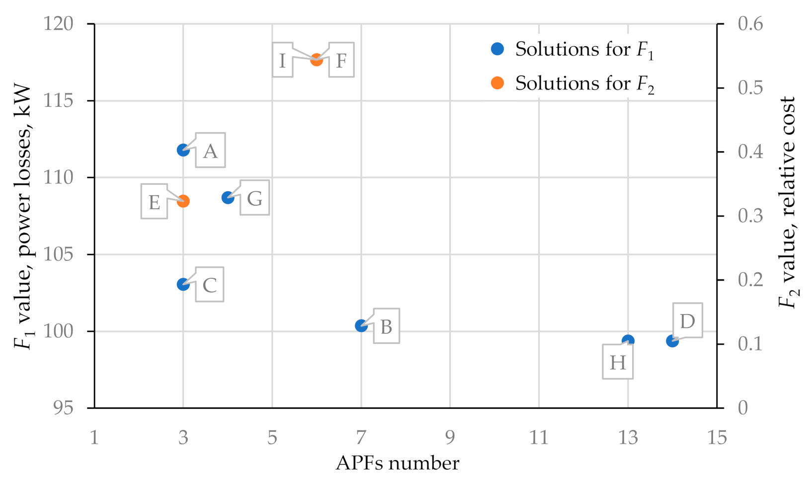
The decision tree algorithm is much faster compared to the brute force algorithm, especially for complex systems, but computation speed is achieved at the price of reduced quality of optimization. Although the decision tree provides results close to globally optimal (see DT solutions in Figure 12), it does not guarantee finding them exactly. Final optimized values of F₁ and F₂ functions for each route, along with the number of placed APFs required for obtaining them, have been presented in Figure 16. As shown, there are solutions that reduce the goal functions highly, but in order to accomplish that effect, a large number of APFs have to be placed in the system. On the other hand, solutions that minimize the goal functions similarly can be found. In this case, the number of required APFs is significantly smaller.

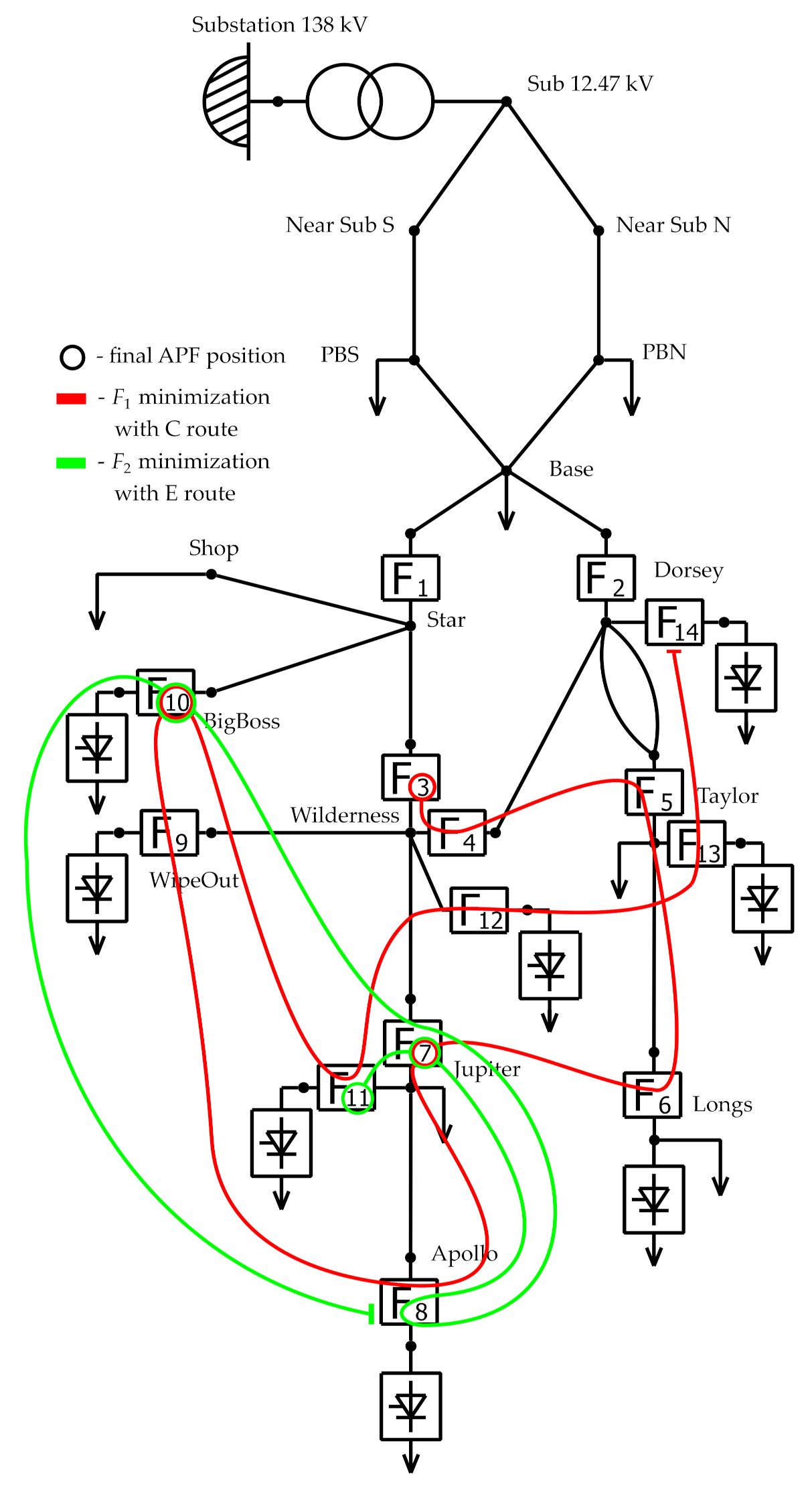
From the set of all examined routes, two examples were chosen in order to provide a more detailed analysis of the decision tree algorithm workflow. The chosen C and E routes are the best compromise between the number of APFs and the goal function values. Each step and the decision made by the algorithm for those routes have been presented in

Table 4. Details of decisions taken by the decision tree algorithm within C and E routes.

	F1 Minimization with C Route		F2 Minimization with E Route
Step	Number of APF	Decision	Number of APF	Decision
1	14	Next	8	Next
2	13	Next	10	Place APF
3	12	Next	7	Previous
4	11	Next	8	Next
5	10	Place APF	7	Place APF
6	9	Next	11	Place APF
7	8	Next	Terminate algorithm
8	7	Place APF
9	6	Next
10	5	Next
11	4	Next
12	3	Place APF
13	Terminate algorithm

. Additionally, all steps taken by the decision tree have been also superimposed graphically on the power system schematic in Figure 17. Both ways of presenting the data provide a clear view on the capabilities of the decision tree algorithm implementation. Although C and E routes result in placing three APFs, they vary by APF sorting method and final results. The different sorting also causes E route to turn around at some point in order to examine a previously checked position but with the first APF already placed. Such behavior was not necessary in C route. Those examples represent different strategies that can be applied by the algorithm during the optimization process.

Table 5. Values of THDVs for all node voltages and THDIs for all line currents for C and E route.

Node	THDV, % C Route	THDV, % E Route	Line	THDI, % C Route	THDI, % E Route
1	0.6	3.3	20-1	0.7	11.0
2	0.6	3.3	1-2	0.7	11.0
3	0.6	3.3	1-3	0.7	11.0
4	0.6	3.4	2-4	0.7	10.9
5	0.6	3.4	3-5	0.7	10.9
6	0.6	3.5	4-6	0.8	12.2
7	0.6	3.7	5-6	0.8	12.2
8	0.6	3.8	6-7	0.0	22.3
9	0.7	3.8	6-9	2.3	19.3
10	0.7	3.8	7-16	0.6	3.4
11	0.9	4.0	7-15	0.0	30.7
12	1.4	4.2	7-8	0.0	16.7
13	0.9	3.8	8-9	12.6	40.2
14	0.8	4.0	8-14	32.8	32.8
15	0.6	3.7	8-13	13.9	23.0
16	0.6	3.7	13-12	29.7	29.7
20	0.1	0.8	9-10	6.9	6.9
			10-11	6.1	6.1

summarizes the voltage total harmonic distortion coefficients (THDVs) for all nodes and current total harmonic distortion coefficients (THDIs) for all lines of the analyzed system in the case of optimization using the decision tree algorithm within C and E routes. A clear improvement of THDVs for all nodes as compared to results without APF (Table 1) can be noticed. However, the results for the optimization within the E road are slightly worse because it was associated with cost minimization (F₂).

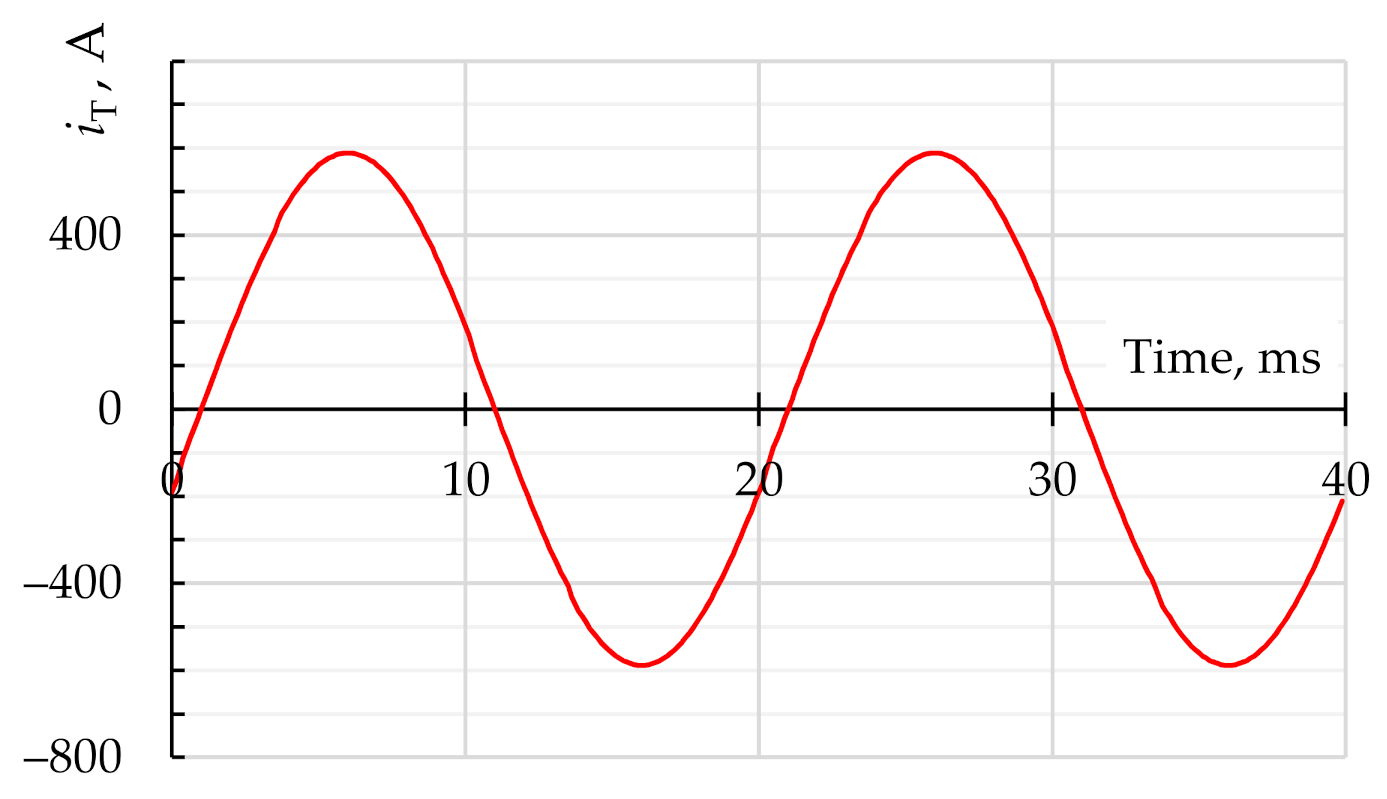
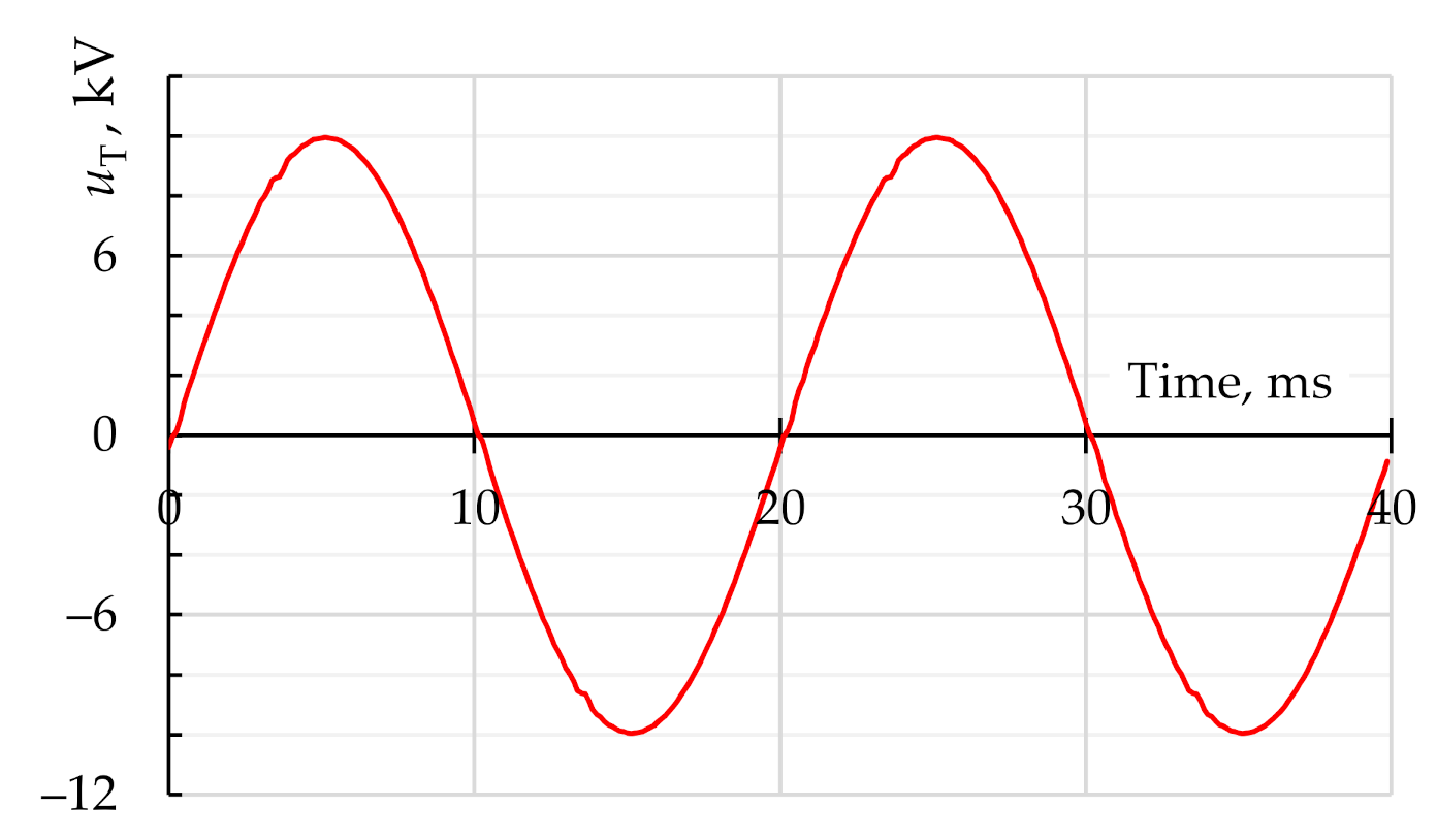
Figure 18, Figure 19, Figure 20 and Figure 21 show the current (sum of currents of line 1-2 and 1-3) and voltage (node no. 1) waveforms of the transformer secondary side. These waveforms can be compared with the waveforms in Figure 6 and Figure 7.

4. Discussion

This paper addresses the problem of optimization of APF placement in an exemplary power system. However, the presented solutions are universal and can be applied to any power system in which the necessity of improvement of power quality occurs due to nonlinear loads or reactive power issues. The research concerned various strategies of the best way of designing a dispersed power quality improvement system. The test circuit used in this paper fulfilled its role in terms of sufficient structural complexity and presence of current and voltage distortions.

The validity of used goal functions was verified. The minimization of power losses has a direct positive effect on power quality in modeled systems. The reduction of power losses through elimination of higher harmonics and reactive power compensation leads to a decrease in THDV levels. This fact contributes to an improvement in economic factors related to excessive power consumption, viability, or restrictions imposed by energy providers. The minimization of power losses along with THDV limitation is connected with the need to install several APFs, which should be placed optimally in order to prevent an unnecessary increase in costs. The minimization of costs is in turn related with the pricing of APFs available in the market. Total costs of a solution depend on rated currents of every APF included in the system, which on the other hand depend on the harmonic distortions and amount of reactive power. Those parameters are strictly connected with placement of APFs in the circuit, and for some solutions, total costs can be the factor that prejudge the final decisions about the power quality improvement system. However, in order to find the best possible outcome, a multi-criterion analysis is necessary. As presented in this paper, there are solutions located in the Pareto frontier that represent a compromise between high price and proper power loss reduction.

The optimization of APF placement described in this paper was conducted using two different methods. The first one is a method consisting in a complete search through all possible solutions (brute force algorithm). Such an approach is the least complex one and has exemplary effectiveness—it always leads to finding the best possible outcome. Despite its efficacy, it is also linked to the necessity of simulating the power system for every possible combination of APF placement, which requires large computation power and time, especially for complex circuits. The second used method was implemented with a premise of reduction of time and algorithm steps leading to a final conclusion. It uses a decision tree algorithm with sorting of the algorithm’s planned route. This approach is highly sensitive for its starting point and configuration of following steps in general. Due to its sensitivity, this paper shows results of analysis for different route sorting strategies. In case of good conditioning of the planned route, the decision tree finds a solution very quickly. The reason is that in comparison to brute force, there are very few simulations that need to be conducted in order to find the best outcome. However, such an outcome may not be the best globally, but as presented in previous chapters, decision tree results are placed close to the Pareto frontier of all solutions in multi-criterion analysis. This paper presents the application of three different approaches to route design for the decision tree. The first is based on indexes assigned to APFs on the schematic and can be captious if the system is designed in an unstructured way. The second one relates to THDV values of nodes where APFs can be installed and sorts them in descending order. The final sorting method relies on the ascending order of APFs currents. As presented, each approach can lead to good results of optimization. Implementing additional conditions regulating the balance between the decision of adding a new APF, instead of moving the current one into better placement, further improves decision tree results. Due to that fact, there is no risk of obtaining trivial solutions such as placing APFs in every possible location in order to minimize power losses as much as possible.

5. Conclusions

The problem of the optimization of harmonic filter allocation in terms of reducing power losses and costs of APFs has been presented in this paper. The emphasis was put on the decision tree algorithm, which is widely known in different research areas, although up to now it has not been commonly applied for power filter allocation in medium-voltage networks. For comparison purposes, a simple brute force algorithm was also implemented. Results indicate that application of the decision tree provide very fast and well-optimized solutions on condition that a route of the algorithm is appropriate. Due to the fact the that decision tree is highly sensitive to its route design, three different approaches of its arrangement have been examined. They consist in sequential analysis of APFs sorted by node THDV value (descending order), APF current value (ascending order), and random manner, which in this case was APF numbers on the schematic (ascending order). The best results obtained from the decision tree were located closely to the Pareto frontier of both power losses and solution cost reduction.

References

1. Ziari, I.; Jalilian, A. Optimal placement of an active filter in a power system. In Proceedings of the 2007 42nd International Universities Power Engineering Conference, Brighton, UK, 4–6 September 2007; pp. 1150–1154. [Google Scholar]
2. Guo, M.; Jin, Q.; Yao, Z. Implementation of Adaptive Step-Size Algorithm in Distribution Network for Optimal Location and Sizing of SAPFs. In Proceedings of the 2020 IEEE/IAS Industrial and Commercial Power System Asia (I&CPS Asia), Weihai, China, 13–16 July 2020; pp. 1562–1566. [Google Scholar]
3. Alhaddad, F.M.; El-Hawary, M. Optimal Filter Placement and Sizing Using Ant Colony Optimization in Electrical Distribution System. In Proceedings of the 2014 IEEE Electrical Power and Energy Conference, Calgary, AB, Canada, 12–14 November 2014; pp. 128–133. [Google Scholar]
4. Shivaie, M.; Salemnia, A.; Ameli, M.T. A multi-objective approach to optimal placement and sizing of multiple active power filters using a music-inspired algorithm. Appl. Soft Comput. 2014, 22, 189–204. [Google Scholar] [CrossRef]
5. Rosyadi, A.; Penangsang, O.; Soeprijanto, A. Optimal filter placement and sizing in radial distribution system using whale optimization algorithm. In Proceedings of the 2017 International Seminar on Intelligent Technology and Its Applications (ISITIA), Surabaya, Indonesia, 28–29 August 2017; pp. 87–92. [Google Scholar] [CrossRef]
6. Lakum, A.; Mahajan, V. Optimal placement and sizing of multiple active power filters for radial distribution system using grey wolf optimizer. In Proceedings of the 2017 7th International Conference on Power Systems (ICPS), Pune, India, 21–23 December 2017; pp. 562–567. [Google Scholar]
7. Sindhu, M.R.; Jisma, M.; Maya, P.; Krishnapriya, P.; Vivek, M.M. Optimal Placement and Sizing of Harmonic and Reactive Compensators in Interconnected Systems. In Proceedings of the 15th IEEE India Council International Conference, Coimbatore, India, 16–18 December 2018; pp. 1–6. [Google Scholar]
8. Belchior, F.N.; De Lima, L.R.; Ribeiro, P.F.; Castro, J.F.C. A novel approach towards passive filter placement. In Proceedings of the 2015 IEEE Power & Energy Society General Meeting, Denver, CO, USA, 26–30 July 2015; pp. 1–5. [Google Scholar]
9. Maciążek, M.; Grabowski, D.; Pasko, M. Genetic and combinatorial algorithms for optimal sizing and placement of active power filters. Int. J. Appl. Math. Comput. Sci. 2015, 25, 269–279. [Google Scholar] [CrossRef] [Green Version]
10. El-Arwash, H.M.; Azmy, A.M.; Rashad, E.M. A GA-based initialization of PSO for optimal APFS allocation in water desali-nation plant. In Proceedings of the Nineteenth International Middle East Power Systems Conference (MEPCON), Cairo, Egypt, 19 December 2017; pp. 1378–1384. [Google Scholar]
11. Milovanović, M.; Radosavljević, J.; Klimenta, D.; Perović, B. GA-based approach for optimal placement and sizing of passive power filters to reduce harmonics in distorted radial distribution systems. Electr. Eng. 2019, 101, 787–803. [Google Scholar] [CrossRef]
12. Moghbel, M.; Masoum, M.A.S.; Fereidouni, A.; Deilami, S. Optimal Sizing, Siting and Operation of Custom Power Devices with STATCOM and APLC Functions for Real-Time Reactive Power and Network Voltage Quality Control of Smart Grid. IEEE Trans. Smart Grid 2018, 9, 5564–5575. [Google Scholar] [CrossRef]
13. Moghbel, M.; Deilami, S.; Masoum, M.A. Optimal Siting and Sizing of Multiple Active Power Line Conditioners to Minimize Network THD Considering Harmonic Couplings. In Proceedings of the 2019 9th International Conference on Power and Energy Systems (ICPES), Perth, Australia, 10–12 December 2019; pp. 1–6. [Google Scholar]
14. Tian, S.; Jia, Q.; Xue, S.; Yu, H.; Qu, Z.; Gu, T. Collaborative optimization allocation of VDAPFs and SVGs for simultaneous mitigation of voltage harmonic and deviation in distribution networks. Int. J. Electr. Power Energy Syst. 2020, 120, 106034. [Google Scholar] [CrossRef]
15. Subramani, C.; Jimoh, A.-G.A.; Dash, S.S.; Harishkiran, S. PSO Application to Optimal Placement of UPFC for Loss Minimization in Power System. In Advances in Intelligent Systems and Computing, Proceedings of the Sproceedings of the 2nd International Conference on IntelPubligent Computshing and Applications, Amsterdam, The Netherlands, 22 February 2017; Springer: Singapore, Singapore, 2017; pp. 223–230. [Google Scholar]
16. Chakeri, V.; Hagh, M.T. Optimal allocation of the distributed active filters based on total loss reduction. Int. J. Smart Electr. Eng. 2017, 6, 171–175. [Google Scholar]
17. Li, D.; Wu, Z.; Zhao, B.; Zhang, X.; Zhang, L. An Adaptive Active Power Optimal Allocation Strategy for Power Loss Minimization in Islanded Microgrids. In Proceedings of the IECON 2019-45th Annual Conference of the IEEE Industrial Electronics Society, Lisbon, Portugal, 14–17 October 2019; Volume 1, pp. 292–297. [Google Scholar]
18. Lopez, J.A.; Lu, C.-N. A comparison of placement methods for collecting PMU data used in angular stability detection. In Proceedings of the 2017 19th International Conference on Intelligent System Application to Power Systems (ISAP), San Antonio, TX, USA, 17–20 September 2017; pp. 1–6. [Google Scholar]
19. Alhalaseh, R.; Tokel, H.A.; Chakraborty, S.; Alirezaei, G.; Mathar, R. Feature-Selection based PMU Placement for Detection of Faults in Power Grids. In Proceedings of the 2018 28th International Telecommunication Networks and Applications Conference (ITNAC), Sydney, NSW, Australia, 21–23 November 2018; pp. 1–6. [Google Scholar]
20. Samudrala, A.N.; Amini, M.H.; Kar, S.; Blum, R.S. Optimal Sensor Placement for Topology Identification in Smart Power Grids. In Proceedings of the 2019 53rd Annual Conference on Information Sciences and Systems (CISS), Baltimore, MD, USA, 20–22 March 2019; pp. 1–6. [Google Scholar]
21. Sevlian, R.A.; Zhao, Y.; Rajagopal, R.; Goldsmith, A.; Poor, H.V. Outage Detection Using Load and Line Flow Measurements in Power Distribution Systems. IEEE Trans. Power Syst. 2018, 33, 2053–2069. [Google Scholar] [CrossRef]
22. Alhalaseh, R.; Tokel, H.A.; Chakraborty, S.; Alirezaei, G.; Mathar, R. PMU Placement with Power Grid Partitioning for Line Outage Detection. In Proceedings of the 2019 4th International Conference on Smart and Sustainable Technologies (SpliTech), Split, Croatia, 18–21 June 2019; pp. 1–6. [Google Scholar]
23. Samudrala, A.N.; Amini, M.H.; Kar, S.; Blum, R.S. Sensor Placement for Outage Identifiability in Power Distribution Net-works. IEEE Trans. Smart Grid 2020, 11, 1996–2013. [Google Scholar] [CrossRef] [Green Version]
24. Sharma, G.; Mahela, O.P.; Kumar, M.; Kumar, N. Detection and Classification of Transmission Line Faults Using Stockwell Transform and Rule Based Decision Tree. In Proceedings of the 2018 International Conference on Smart Electric Drives and Power System (ICSEDPS), Nagpur, India, 12–13 June 2018; pp. 1–5. [Google Scholar]
25. Godse, R.; Bhat, S. Mathematical Morphology-Based Feature-Extraction Technique for Detection and Classification of Faults on Power Transmission Line. IEEE Access 2020, 8, 38459–38471. [Google Scholar] [CrossRef]
26. Gong, C.-S.A.; Su, C.-H.S.; Tseng, K.-H. Implementation of Machine Learning for Fault Classification on Vehicle Power Transmission System. IEEE Sens. J. 2020, 20, 15163–15176. [Google Scholar] [CrossRef]
27. Ribeiro, E.G.; Dias, G.L.; Barbosa, B.H.G.; Ferreira, D.D. Real-time system for automatic classification of power quality dis-turbances. In Proceedings of the 17th International Conference on Harmonics and Quality of Power (ICHQP), Belo Horizonte, Brazil, 16–19 October 2016; pp. 908–913. [Google Scholar]
28. Shams, N.; Wall, P.; Terzija, V. Active Power Imbalance Detection, Size and Location Estimation Using Limited PMU Meas-urements. IEEE Trans. Power Syst. 2019, 34, 1362–1372. [Google Scholar] [CrossRef]
29. Meng, X.; Zhang, P.; Zhang, D. Decision Tree for Online Voltage Stability Margin Assessment Using C4.5 and Relief-F Algorithms. Energies 2020, 13, 3824. [Google Scholar] [CrossRef]
30. Jindal, A.; Dua, A.; Kaur, K.; Singh, M.; Kumar, N.; Mishra, S. Decision Tree and SVM-Based Data Analytics for Theft Detection in Smart Grid. IEEE Trans. Ind. Inform. 2016, 12, 1005–1016. [Google Scholar] [CrossRef]
31. Guerrero, J.I.; Monedero, I.; Biscarri, F.; Biscarri, J.; Millan, R.; Leon, C. Non-Technical Losses Reduction by Improving the Inspections Accuracy in a Power Utility. IEEE Trans. Power Syst. 2017, 33, 1209–1218. [Google Scholar] [CrossRef]
32. Swetapadma, A.; Yadav, A. A Novel Decision Tree Regression-Based Fault Distance Estimation Scheme for Transmission Lines. IEEE Trans. Power Deliv. 2017, 32, 234–245. [Google Scholar] [CrossRef]
33. Pessoa, A.L.D.S.; Oleskovicz, M.; Martins, P.E.T. A multi-stage methodology for fault location in radial distribution systems. In Proceedings of the 2018 18th International Conference on Harmonics and Quality of Power (ICHQP), Ljubljana, Slovenia, 13–16 May 2018; pp. 1–6. [Google Scholar]
34. Araújo, M.A.; Flauzino, R.A.; Moraes, L.A.; Borges, F.A.S.; Spatti, D.H. Decision Trees Applied to Fault Locations in Distri-bution Systems with Smart Meters. In Proceedings of the IEEE International Conference on Environment and Electrical Engi-neering and 2019 IEEE Industrial and Commercial Power Systems Europe (EEEIC/I&CPS Europe), Genova, Italy, 11–14 June 2019; pp. 1–6. [Google Scholar]
35. Xiong, P.; Singh, C. Optimal Planning of Storage in Power Systems Integrated with Wind Power Generation. IEEE Trans. Sustain. Energy 2016, 7, 232–240. [Google Scholar] [CrossRef]
36. Lee, C.-T.; Horng, S.-C. Abnormality Detection of Cast-Resin Transformers Using the Fuzzy Logic Clustering Decision Tree. Energies 2020, 13, 2546. [Google Scholar] [CrossRef]
37. Sai, T.; Kumar, P.S.; Reddy, K. Towards intelligent decision making in power plant operation. In Proceedings of the 2014 Annual IEEE India Conference (INDICON), Puni, India, 11–13 December 2014; pp. 1–6. [Google Scholar]
38. Mosavi, A.; Salimi, M.; Ardabili, S.F.; Rabczuk, T.; Shamshirband, S.; Varkonyi-Koczy, A.R. State of the Art of Machine Learning Models in Energy Systems, a Systematic Review. Energies 2019, 12, 1301. [Google Scholar] [CrossRef] [Green Version]
39. Leonidaki, E.; Georgiadis, D.; Hatziargyriou, N. Decision Trees for Determination of Optimal Location and Rate of Series Compensation to Increase Power System Loading Margin. IEEE Trans. Power Syst. 2006, 21, 1303–1310. [Google Scholar] [CrossRef]
40. Couronné, R.; Probst, P.; Boulesteix, A.-L. Random forest versus logistic regression: A large-scale benchmark experiment. BMC Bioinform. 2018, 19, 1–14. [Google Scholar] [CrossRef] [PubMed]
41. Ke, G.; Meng, Q.; Finley, T.; Wang, T.; Chen, W.; Ma, W.; Ye, Q.; Liu, T.Y. Lightgbm: A highly efficient gradient boosting decision tree. Adv. Neural Inf. Process. Syst. 2017, 30, 3146–3154. [Google Scholar]
42. Tian, W.; Lei, C.; Tian, M. Dynamic Prediction of Building HVAC Energy Consumption by Ensemble Learning Approach. In Proceedings of the 2018 International Conference on Computational Science and Computational Intelligence (CSCI), Las Vegas, Nevada, USA, 13–15 December 2018; pp. 254–257. [Google Scholar]
43. Grady, W.M. Understanding Power System Harmonics. Available online: http://web.ecs.baylor.edu/faculty/grady/ (accessed on 18 January 2021).
44. Buła, D.; Lewandowski, M. Steady state simulation of a distributed power supplying system using a simple hybrid time-frequency model. Appl. Math. Comput. 2018, 319, 195–202. [Google Scholar] [CrossRef]
45. Buła, D.; Grabowski, D.; Lewandowski, M.; Maciążek, M.; Piwowar, A. Software Solution for Modeling, Sizing, and Allocation of Active Power Filters in Distribution Networks. Energies 2020, 14, 133. [Google Scholar] [CrossRef]
46. Buła, D.; Lewandowski, M. Comparison of frequency domain and time domain model of a distributed power supplying system with active power filters (APFs). Appl. Math. Comput. 2015, 267, 771–779. [Google Scholar] [CrossRef]
Figure 1. Bar graph of exemplary relative costs of active power filters (APFs) depending on their rated current.
Energies 14 01173 g001
Figure 2. Block diagram of the brute force algorithm.
Energies 14 01173 g002
Figure 3. Schematic of recurring part of decision tree used for the optimization of APF placement.
Energies 14 01173 g003
Figure 4. Diagram of the test power system with marked possible locations of APFs (F1–F14).
Energies 14 01173 g004
Figure 5. Model of active power filter.
Energies 14 01173 g005
Figure 6. Current waveform of the secondary side of the transformer in the analyzed system.
Energies 14 01173 g006
Figure 7. Voltage waveform of the secondary side of the transformer in the analyzed system.
Energies 14 01173 g007
Figure 8. Dependence of the number of cases and the calculation time of the brute force algorithm on the APF number.
Energies 14 01173 g008
Figure 9. Values of the goal functions depending on the number of optimally placed APFs; (a) for F1; (b) for F2.
Energies 14 01173 g009aEnergies 14 01173 g009b
Figure 10. Bar chart of the maximum THDV value among all network nodes for the allocation of two APFs.
Energies 14 01173 g010
Figure 11. Objective function values for all feasible solutions in the case of three APFs installed in the system (MTHDV—number of feasible solutions, MNP—number of noninferior points).
Energies 14 01173 g011
Figure 12. Objective function values for all solutions in the case of three APFs installed in the system (M—total number of solutions, MTHDV—number of feasible solutions, MNP—number of noninferior points).
Energies 14 01173 g012
Figure 13. Objective function and THDV values for all solutions in the case of three APFs installed in the system (M—total number of solutions, MTHDV—number of feasible solutions, MNP—number of noninferior points).
Energies 14 01173 g013
Figure 14. Maximum THDV, F1, and F2 values for each decision tree algorithm step for F1 minimization; (a) A and B routes; (b) C and D routes; (c) G and H routes.
Energies 14 01173 g014aEnergies 14 01173 g014b
Figure 15. Maximum THDV, F1, and F2 values for each decision tree algorithm step for F2 minimization; (a) E route; (b) F route; (c) I route.
Energies 14 01173 g015aEnergies 14 01173 g015b
Figure 16. Optimized values of F1 and F2 functions for each route A–H (Table 3) along with the number of placed APFs required for obtaining them.
Energies 14 01173 g016
Figure 17. Graphical representation of C and E routes of the decision tree algorithm with final positions of APFs.
Energies 14 01173 g017
Figure 18. Current waveform of the secondary side of the transformer in the analyzed system in the case of optimization using the decision tree algorithm within C route.
Energies 14 01173 g018
Figure 19. Voltage waveform of the secondary side of the transformer in the analyzed system in the case of optimization using the decision tree algorithm within C route.
Energies 14 01173 g019
Figure 20. Current waveform of the secondary side of the transformer in the analyzed system in the case of optimization using the decision tree algorithm within E route.
Energies 14 01173 g020
Figure 21. Voltage waveform of the secondary side of the transformer in the analyzed system in the case of optimization using the decision tree algorithm within E route.
Energies 14 01173 g021