Simulation of Low Inertia Power Systems Based on Shifted Frequency Analysis

Abstract

New types of power system transients with lower time constants are emerging due to the replacement of synchronous generation with converter interfaced generation and are challenging the modeling approaches conventionally applied in power system simulation. Quasi-stationary simulations are based on classical phasor models, whereas EMT simulations calculate the instantaneous values of models in the time domain. In addition to these conventional modeling approaches, this paper investigates simulation based on dynamic phasor models, as has been proposed by the Shifted Frequency Analysis. The simulation accuracy of the three modeling approaches was analyzed for characteristic transients from the electromagnetic to the electromechanical phenomena range, including converter control as well as low inertia transients. The analysis was carried out for systems with converter interfaced and synchronous generation whilst considering the simulation step size as a crucial influence parameter. The results show that simulations based on dynamic phasors allow for larger step sizes than simulations that calculate the instantaneous values in the time domain. This can facilitate the simulation of more complex component models and larger grid sizes. In addition, with dynamic phasors, more accurate simulation results were obtained than with classical phasors, in particular—but not exclusively—in a low inertia case. Overall, the presented work demonstrates that dynamic phasors can enable fast and accurate simulations during the transition to low inertia power systems.

1. Introduction

The ongoing energy transition involves the migration from conventional power plants to renewable energy resources. The replacement of synchronous generation by converter interfaced generation is leading to the appearance of new types of power system dynamics. A major concern of transmission system operators is the decrease in the system’s inertia, as it causes new types of transients with lower time constants and can raise stability issues due to significant frequency fluctuations.

In this context, this paper investigated the potential implications for power system simulations. The modeling approach employed for power system simulation depends on the type of phenomenon being analyzed. In general, dynamic phenomena in power systems are categorized according to their time constants. Electromagnetic phenomena are characterized by smaller time constants in the range of microseconds. These phenomena emerge, e.g., due to switching actions or power electronics equipment, and are simulated with programs that calculate the instantaneous values of the waveforms in the time domain. The simulation based on time domain models is called Electromagnetic Transient (EMT) simulation. However, these simulations require small simulation steps in the microsecond range to ensure the accuracy of the waveforms. Hence, EMT simulations require significant computational efforts and are typically limited to small-scale studies.

Instead, electromechanical phenomena are characterized by larger time constants in the range from milliseconds to seconds. They are related to large rotating generation units. Due to the larger time constants, the numerical calculation of electromechanical phenomena is commonly based on classical phasor models. This approach is called quasi-stationary simulation. It enables the choice of larger simulation step sizes and the execution of large-scale simulations.

To date, electromagnetic and electromechanical phenomena have mostly been considered in a decoupled way, resulting in the adoption of EMT or quasi-stationary simulations. However, the new dynamics emerging in power systems in the presence of converter interfaced generation and low system inertia may fall in the range between these two categories. To bridge the scales of electromagnetic and electromechanical transient phenomena, the concept of Shifted Frequency Analysis (SFA) has been proposed [1,2]. The main idea is to change the modeling paradigm that is behind the existing simulation approaches. In SFA, power system components are modeled by means of time-varying phasors, also referred to as dynamic phasors.

In contrast to the calculation of instantaneous values in the time domain, as done in EMT simulations, SFA calculates one or more dynamic phasors to represent the transients without including their predominant carrier frequencies. This is achieved by the shift of the original frequency spectrum and enables the choice of larger simulation step sizes to improve the computational speed [3]. Consequently, it facilitates the simulation of large-scale systems and reduces the requirements on the simulation hardware.

In contrast to classical phasor models applied in quasi-stationary simulations, dynamic phasor models can also deliver accurate simulation results when attempting the simulation of transients with lower time constants. This is because dynamic phasors are capable of representing the dynamic behavior between two consecutive network states, while classical phasors imply fully electromagnetically decoupled network states [4].

Overall, SFA-based simulations with dynamic phasors can enable both fast and accurate simulations for modern power systems. For example, improved accuracy with respect to quasi-stationary simulations can ensure the reliability of the online dynamic security assessment performed by transmission system operators during network operation. In addition, the application of SFA can support the development of simulation-based digital twins. Digital twins are envisioned to support hardware developments by interfacing newly developed devices to power system digital twins. However, this Hardware-In-the-Loop (HIL) testing requires the execution of simulations in real-time, that is, the computations must be completed within deterministic time intervals. To achieve such deterministic computation times, real-time solvers, as employed in this work, choose a fixed simulation step size. SFA simulations allow the user to increase the simulation step size with respect to EMT simulations, which in turn enables longer computation time intervals. This facilitates the solution of more complex component models and larger grid sizes.

With such potential applications, this work investigated the capability of dynamic phasors applied in SFA to represent the characteristic transients emerging in modern power systems. The use of dynamic phasors was compared with the employment of classical phasors in quasi-stationary simulations and time domain models in EMT simulations. The performance of the modeling approaches was assessed in terms of the resulting simulation accuracy and the required simulation step size. We considered cases of electromagnetic and electromechanical transients as well as of converter control and low synchronous inertia transients. The simulations based on the three modeling approaches were run in one single simulator, namely the dynamic power system simulator DPsim [5]. The simulator is developed as open source software project. Hereby, we intend to make all models applied within this work available to other researchers for further investigations.

In Section 2, we present related work already carried out in the field of SFA. Section 3 provides the theoretical background of this work with a focus on a comparative presentation of the fundamentals behind the modeling approaches. Section 4 describes the implementation of the test systems together with the applied component models, while the corresponding results are presented and discussed in Section 5.

2. Related Work

Shifted Frequency Analysis (SFA) has been employed to increase the simulation step size in Electromagnetic Transients Programs (EMTPs) while ensuring accurate simulation results [6]. In addition, it has been applied to improve the simulation efficiency of asymmetrical fault simulations and simulations under unbalanced conditions [7,8]. In addition, dynamic phasors have been used as a unified modeling approach to capture transients from the electromagnetic to the electromechanical range by an automatic and adaptive choice of the simulation step size [9,10]. In this context, detailed dynamic phasor models of synchronous machines [11,12], induction machines [13,14] and power electronics devices [15,16] have been presented.

Apart from using dynamic phasors as a modeling approach within newly developed simulators, they have also been considered for the interconnection of geographically distributed real-time EMT simulators [17]. By extracting dynamic phasors from EMT signals, latencies caused by communication over long distances have been compensated by a corresponding phase shift applied to the dynamic phasors.

Of particular interest are recent case studies that started to focus on the comparison of dynamic phasor based simulations with quasi-stationary simulations. The authors in [18] presented a case study on the Irish transmission grid. They were able to show an improved simulation accuracy in terms of frequency and voltage when running dynamic phasor based simulations. In addition, two case studies on common benchmark systems have been reported in [19]. The authors were able to demonstrate the high accuracy of the transient stability assessment with dynamic phasors considering the critical clearing time.

In this context, our work compares SFA-based simulations with both EMT and quasi-stationary simulations at the same time. This places emphasis on the simulation accuracy of the transients themselves rather than considering system-level criteria such as the critical clearing time. It analyzes the characteristic types of transients emerging in low inertia power systems. In contrast to other studies, the simulation step size is not set to specific values but varied systematically over a wide range to analyze its impact on the simulation accuracy and to allow for the identification of suitable step sizes for each type of transient and modeling approach.

3. Theoretical Background

This section presents in a comparative manner the fundamental theoretical differences between the modeling approaches in quasi-stationary, SFA and EMT simulations. To begin with the fundamentals behind quasi-stationary simulations, a sinusoidal signal of a single frequency being fully periodic in the time interval of a simulation step $t\in [t_0,t_0+\Delta t]$ is expressed as

$$x\left(t\right)=Acos(\omega t+\theta )$$

(1)

A is the amplitude, $\omega$ is the signal’s frequency and $\theta$ is the initial phase angle. It is common practice to represent such sinusoidal signals by means of complex quantities with a corresponding imaginary part. That is, we can express $x\left(t\right)$ by

$$x\left(t\right)=\mathit{Re}\left\{A{e}^{j\theta }{e}^{j\omega t}\right\}$$

(2)

The complex term $A{e}^{j\theta }$ is constant in time and commonly denoted as a phasor:

$$X_1:=A{e}^{j\theta }$$

(3)

In this work, we also refer to it as a classical phasor or, due to its characteristic of being constant in time, as a Static Phasor (SP). SPs are widely used in power flow and quasi-stationary simulations. The crucial advantage of SP-based calculations is the omission of the $e^{j\omega t}$ term. From a simulation perspective, it is particularly advantageous that the oscillation with the fundamental frequency is omitted by static phasors. This avoids the necessity of small simulation step sizes, as the step size needs to be adapted to the oscillations with the highest frequency [20].

In time series power flow and quasi-stationary simulations, for each simulation step a new static phasor is calculated according to the current conditions of the grid, e.g., according to the current operation points of generators and loads. For each simulation step, static phasors enforce that the grid is in a steady state and that the signals are fully periodically oscillating with a fixed frequency. The fixed frequency can be considered either as constant over the entire simulation, usually assuming the nominal frequency of the grid, or as varying from simulation step to simulation step, by calculating a system-wide frequency, e.g., the Center Of Inertia (COI), potentially leading to more accurate results [21]. Nevertheless, in both cases, static phasors are subject to the restriction that the grid signals have a fixed frequency within one simulation step.

In harmonic analysis, the concept of static phasors is extended to signals with integer multiples of the fundamental frequency. Accordingly, real-value signals are represented by a set of complex static phasors $X_k$ according to:

$$x\left(t\right)=\mathit{Re}\left\{\sum _k{X}_k{e}^{jk\omega t}\right\}$$

(4)

However, the assumption of the presence of signals with an amplitude and phase constant in time is to be questioned, particularly in power systems with a significant presence of converter-based components [22]. More signal dynamics, in particular higher frequency fluctuations, will have to be reflected within an interval $t\in [t_0,t_0+\Delta t]$. However, the more accurate simulation of the time domain waveforms in EMT simulations suffers from the requirement of small simulation step sizes.

The idea behind the application of Shifted Frequency Analysis (SFA) is that signals emerging in power systems with a high penetration of renewable energy resources will still have a limited bandwidth around the fundamental frequency, i.e., they can be represented as bandpass in the frequency spectrum. Accordingly, signals of the following form are assumed:

$$\tilde{x}\left(t\right)=A\left(t\right)cos(\omega t+\theta \left(t\right))$$

(5)

A time-varying $A\left(t\right)$ allows for an amplitude modulation of the sinusoidal signal, while a time-varying $\theta \left(t\right)$ enables a phase modulation, which can also reflect a frequency modulation. For bandpass signals, these modulations will be in the low-frequency range. Mathematically, we can describe the signal $\tilde{x}\left(t\right)$ again by means of complex quantities according to:

$$\tilde{x}\left(t\right)=\mathit{Re}\left\{A\left(t\right)e^{j\theta \left(t\right)}{e}^{j\omega t}\right\}$$

(6)

The corresponding phasor is time-varying

$${\tilde{X}}_1\left(t\right):=A\left(t\right)e^{j\theta \left(t\right)}$$

(7)

and hence, referred to as Dynamic Phasor (DP). Again, it should be noted that ${\tilde{X}}_1\left(t\right)$ does not include the fundamental frequency oscillations due to the omission of $e^{j\omega t}$. In other words, the frequency spectrum of ${\tilde{X}}_1\left(t\right)$ is shifted by the fundamental frequency $\omega$, due to which DP-based considerations are also named Shifted Frequency Analysis (SFA). DPs allow for nearly periodic signals in contrast to the fully periodic signals imposed by SPs, as DPs are capable of representing the amplitude and phase variations of a limited bandwidth around the fundamental frequency, whereas SPs are restricted within one simulation interval to constant amplitude and phase values.

Especially in power systems with an increased amount of power electronics devices, more and more harmonics occur due to the devices’ switching characteristic. These harmonics can be represented with a set of dynamic phasors according to:

$$\tilde{x}\left(t\right)=\mathit{Re}\left\{\sum _k{\tilde{X}}_k\left(t\right)e^{jk\omega t}\right\}$$

(8)

This is well suited for the representation of multiple bandpasses, where the center frequencies $k\omega$ around which the spectrum is located are significantly higher than the bandwidth of the surrounding frequency bands.

Independently from whether the signals are modeled by means of static or dynamic phasors, they are input to and transmitted via the power system. The power system is a dynamical system that can be modeled by a Differential-Algebraic System of Equations (DAE) according to:

$$F(t,x\left(t\right),\dot{x}\left(t\right))=0$$

(9)

The simulation with static or dynamic phasors requires the transformation of the power system’s DAE to the respective modeling domain. Hence, we subsequently show this transformation and give the basic example of a transmission line model for illustration purposes.

We introduce the notations ${\langle ·\rangle }_{SP}$ and ${\langle ·\rangle }_{DP}$ to express the transformation to the respective modeling domain. Correspondingly, a static phasor is denoted as ${\langle x\left(t\right)\rangle }_{SP}$ while a dynamic phasor is denoted as ${\langle x\left(t\right)\rangle }_{DP}$. The derivation of Equation (4) yields:

$$\frac{dx\left(t\right)}{dt}=\mathit{Re}\left\{\sum _{k}jk\omega X_k{e}^{jk\omega t}\right\}$$

(10)

and provides the required transformation of the derivative $\dot{x}\left(t\right)$ in Equation (9) to the SP domain as follows:

$${\langle \dot{x}\left(t\right)\rangle }_{k,SP}=jk\omega {\langle x\left(t\right)\rangle }_{k,SP}$$

(11)

As an example, a transmission line can be modeled as a series combination of resistance R and inductance L according to the following physical DAE in the time domain:

$$v\left(t\right)-Ri\left(t\right)-L\frac{di\left(t\right)}{dt}=0$$

(12)

Using Equation (11), the transformation of Equation (12) to the SP domain (k = 1) is:

$${\langle v\left(t\right)\rangle }_{1,SP}-R{\langle i\left(t\right)\rangle }_{1,SP}-j\omega L{\langle i\left(t\right)\rangle }_{1,SP}=0$$

(13)

Analogously, the time derivative $\dot{x}\left(t\right)$ transformed to the DP domain is obtained from the derivation of Equation (8) by

$$\frac{d\tilde{x}\left(t\right)}{dt}=\mathit{Re}\left\{\sum _k\left(\frac{d{\tilde{X}}_k\left(t\right)}{dt}+jk\omega {\tilde{X}}_k\left(t\right)\right)e^{jk\omega t}\right\}$$

(14)

This results in the following rule for the transformation of the derivative $\dot{x}\left(t\right)$ to the DP domain:

$${\langle \dot{x}\left(t\right)\rangle }_{k,DP}=\frac{d{\langle x\left(t\right)\rangle }_{k,DP}}{dt}+jk\omega {\langle x\left(t\right)\rangle }_{k,DP}$$

(15)

By applying Equation (15) to Equation (12), the transmission line model appears in the DP domain (k = 1) as follows:

$${\langle v\left(t\right)\rangle }_{1,DP}-R{\langle i\left(t\right)\rangle }_{1,DP}-L\frac{d{\langle i\left(t\right)\rangle }_{1,DP}}{dt}-j\omega L{\langle i\left(t\right)\rangle }_{1,DP}=0$$

(16)

Dynamic phasor models of additional more complex linear and nonlinear grid components are available in related research works, as summarized in the previous section.

4. Implementation

In the frame of this work, we considered two test systems in which fundamental transients with different time constants occurred, and we analyzed the capability of the modeling approaches to accurately represent the transients. We incorporated both Converter Interfaced Generation (CIG) and Synchronous Generation (SG) units, causing characteristic power system transients. The transients cover time constants from the electromagnetic to the electromechanical range and include converter control and low inertia dynamics.

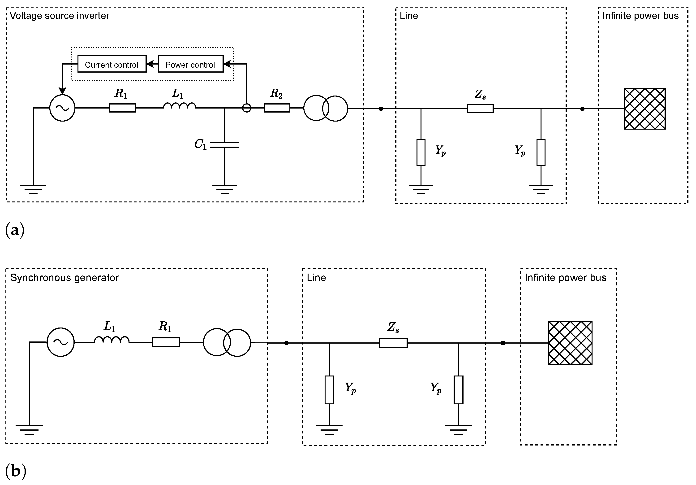
The test systems are shown in Figure 1. Each test system includes a generation unit, either CIG or SG, that injects power. The power is transmitted via a line, implemented as a pi line model, while the rest of the system is represented by an infinite power bus. Thus, we adopted the Single Machine Infinite Bus (SMIB) system, well known in machine studies. We chose these elementary test systems to be able to analyze the transients related to each type of generation unit in a dedicated manner. The emerging transients are easy to understand and their analysis shall provide a basis for further investigations of larger systems with more complex topologies and transients. During the simulation, the characteristic dynamic behavior of the generation units was triggered by load change and fault events at their terminals. In the following, we explain the employed model for each type of generation unit.

4.1. CIG System

As one kind of power electronic equipment interfacing a CIG unit with power systems, we considered a Voltage Source Inverter (VSI). The VSI converts the unit’s generated DC power to AC power. In this work, the VSI’s switching behavior was taken into account by an averaged switching model. In addition to the voltage source, the VSI model includes an $LC$ output filter composed of inductive, capacitive and resistive components, as shown in Figure 1a. In addition, a step-up transformer increases the output switching voltage, here $1.5 \mathrm{k}\mathrm{V}$, to the nominal grid voltage at a medium voltage level of $20 \mathrm{k}\mathrm{V}$.

As depicted in Figure 1a, a control system regulates the voltage source set-point to operate the VSI in grid feeding mode [23]. The control targets the injection of reference values for active and reactive power. An average power calculation of the actual power feed-in serves as input to the outer power control loop implemented as a PI controller. Its output is connected to the inner current control loop, also implemented as a PI controller, which calculates the set-point to the controlled voltage source. Further details on the VSI model have already been presented in [5].

The electrical components were modeled in their respective modeling domains, i.e., in SP, DP or EMT domain. The control components were instead implemented as a state space model with quantities in the local dq reference frame rotating with the frequency measured by a Phase-Locked Loop (PLL). The interface connecting the electrical components with the control components depends on the chosen modeling domain. Hence, [5] describes how control components in the dq frame can be interfaced with electrical components in the EMT and phasor domains.

We would like to stress that we do not claim generality here by considering a power controlled VSI interfacing the CIG unit. Other types of power electronic equipment, e.g., with different types of control such as frequency control, yield other types of characteristic transients. Nonetheless, the considered implementation shall give an indication on how simulations associated with a certain modeling domain are affected by CIG units.

4.2. SG System

For the test system with the SG unit, as shown in Figure 1b, we applied the classical synchronous generator model in accordance with the common practice for transient stability analysis, which consists of a voltage source of constant magnitude and varying phase behind a transient reactance and series resistance [24]. Since our focus here lies with the electromechanical behavior, characterized by larger time constants, no high order model is necessary. The classical model is valid for the initial time period of an electromechanical transient, which is equal to the period of the first swing of the rotor angle $\delta$ [25] and which is the time period of interest in our case. In general, this simplified model offers high computational efficiency allowing large-scale simulations and simultaneously delivers accurate results for the initial period of rotor angle dynamics.

These dynamics are observed after a disturbance and are described by the second order differential swing equation. In order to improve the accuracy and include the damping effects of the rotor damper windings, neglected in the classical model, an electrical damping torque was considered in the swing equation. The main SG control systems, i.e., the turbine governor and the automatic voltage regulator, were neglected in this work. For our simulations, we first applied the actual inertia constant of H equal to 5 s of a 500 MVA machine to model a conventional dynamic behavior, then we decreased H to understand the behavior of low inertia systems.

4.3. Simulation Tool

The aforementioned test systems were implemented within the simulation tool DPsim (https://dpsim.fein-aachen.org, accessed on 26 March 2021) [5]. The simulator targets a detailed simulation of dynamics in real-time while running on commercial off-the-shelf hardware. For this, the simulator introduces the usage of DP models according to SFA. In addition, the component library of DPsim includes models in the SP and EMT domain. We were thus capable of running all the simulations executed in the different modeling domains within the same simulation tool and avoid, e.g., having to perform SP simulations in one simulation tool and EMT simulations in another. On the one hand, this ensures a solid comparison of the modeling domains because the transformed models are based on exactly the same physical models, i.e., on exactly the same DAE describing the physics of the component. On the other hand, the application of a single simulation tool guarantees that the same solution approach, i.e., the same solver, is applied to all models. The simulator is designed for real-time simulation requiring the computations to be executed within a deterministic time interval, and hence, employs a fixed-step solver. The solution of the electrical network is calculated according to the Modified Nodal Analysis (MNA), while the dynamic behavior of the components is considered by means of the components’ DC equivalents applying trapezoidal numerical integration [26]. Depending on the modeling domain under investigation, the DC equivalents represent the models either in the SP, DP or EMT domain.

5. Results and Discussion

In this work, we determined the simulation accuracy of SP, DP and EMT modeling by calculating the Root Mean Squared Error (RMSE) between the occurring transients. Four types of transients with different time constants were considered: electromagnetic and electromechanical transients as well as converter control and low inertia transients. We thus included transients occurring in conventional as well as modern power systems with an increasing amount of renewable energy resources. The transients were investigated in the test systems with the CIG or SG unit, as presented in Section 4. Since simulation accuracy and simulation step size are closely linked to each other, we incorporated the step size throughout the entire analysis as a crucial influence parameter.

5.1. Electromagnetic Transients in CIG System

First, the CIG system described in Section 4.1 was simulated for the case of a VSI with an open control loop. Thus, the set-point of the controlled voltage source remained constant at its initially determined steady-state value. As a consequence, the transients remained unaffected by the control system and solely included electromagnetic dynamics.

The transient response was triggered by the event of a sudden load change. After 5 s of simulation time, a nominal load of 10 MV connected to the VSI terminals representing a severe disturbance in the medium voltage level. The resulting voltage transient at the VSI terminals is shown in black in Figure 2a. The transient was obtained from an EMT simulation with a step size of 50 μs, which will serve as a reference simulation in the following. Figure 2a shows that the transient incorporated a significant voltage dip which is categorizable as an electromagnetic transient given its time constant in the microseconds range.

For small step sizes, the simulation in the DP domain yielded similar results as the simulation in the EMT domain, as shown in Figure 2a for a step size of 100 μs. In contrast to this, the simulation in the SP domain did not reflect the significant voltage dip after the load change. This is because such fast electromagnetic transients are not captured by SP models, even for small step sizes. It should be noted that here, by applying Equations (2) and (6), we transformed SP and DP results back to the time domain so that they can be easily compared with the EMT results.

For large step sizes, as it is depicted in Figure 2b for a step size of 10 ms, it is clearly visible that the simulation results in the EMT domain become unusable due to their high inaccuracy. This is due to the fact that the oscillations with the fundamental frequency of 50 Hz are not captured accurately for such large step sizes.

Figure 3 shows the impact of the simulation step size on the simulation error in more detail when considering step sizes from 100 μs to 10 ms. The RMSE was calculated for each simulation with respect to the reference simulation within the time period of interest, which is in the case of the electromagnetic transient from 4.999 s to 5.05 s. Figure 3 demonstrates that below a step size of 1 ms the simulation accuracy in the DP and EMT domain is the same, while the simulation results in the SP domain are significantly less accurate. This is because, when using the SP modeling approach, the electromagnetic transient cannot be captured.

For step sizes larger than 1 ms, the simulation accuracy deteriorates in the EMT domain. Instead, the simulation error in the DP and SP domain is similar and remains lower than in the EMT domain. This is because the oscillation of the fundamental frequency is predominant after the electromagnetic transient, as it can be seen in Figure 2. As explained in Section 3, these fully periodic oscillations can be reproduced with DPs and SPs in the same way, i.e., by means of phasors that do not incorporate the fundamental frequency oscillations during simulation. In contrast, the simulation in the EMT domain includes the simulation of the fundamental frequency oscillation. Due to this, the EMT accuracy deteriorates significantly for larger step sizes, as shown in Figure 3. This is in line with the findings from EMTP research, according to which the simulation error increases significantly as of 2 ms for 50 Hz oscillations when using the trapezoidal rule for numerical integration [20].

The results show that the user can choose between DP and EMT domain to simulate the electromagnetic transient, while as expected, the SP domain is the wrong modeling choice given that it is incapable of representing the electromagnetic dynamics. The equality of the results in the DP and EMT domain for small step sizes originates from the high bandwidth of the transient, due to which the DPs’ frequency shift by the fundamental frequency of 50 Hz does not have a significant impact. As visible in Figure 3, the simulation step size for DP and EMT should be chosen to be at least below 600 μs to include the electromagnetic dynamics, while as expected, a smaller step size yields a higher accuracy.

5.2. Control Transients in CIG System

Then, we closed the control loop of the VSI in order to examine the accuracy of the modeling domains when the user intends to simulate the control transient. Figure 4 illustrates the control behavior by comparing the closed with the open control loop case. This shows that the control transient has a larger time constant than the electromagnetic transient and lasts several seconds. Before the load step event, the CIG unit generates an active power of 100 kW and a reactive power of $50 \mathrm{kVAr}$ according to the control set-points specified in this scenario. After the load change and in the absence of the control, the VSI’s active and reactive power output consequentially significantly deviated from the set-point values. Instead, closing the control loop caused the VSI to return to the specified set-points with an oscillatory but damped control transient.

In Figure 5, the impact of the control on the VSI’s current transient is shown. It delineates the time period of the control transient from 5.05 s to 6.5 s, whereas the time period of the electromagnetic transient was left out at this point for a dedicated focus on the control transient. Choosing a small step size, 100 μs in Figure 5a, the control transient can be accurately represented in all modeling domains. As can be noticed, in the case of accurate simulations, the depicted magnitudes of the static and dynamic phasors show up as the envelope of the EMT domain transient. This illustrates that here both phasor modeling approaches can represent the amplitude modulation as key signal information caused by the control, while they avoid simulating the oscillations with the fundamental frequency, as it is done in EMT simulations.

When choosing a larger step size, the simulation of the control transient loses accuracy in the EMT domain, as can be seen in Figure 5b for a step size of 700 μs, whereas the simulations in the SP and DP domain remained accurate for this step size. When further increasing the step size to 2 ms, Figure 5c demonstrates that the simulation in the DP domain also loses accuracy due to superimposed oscillations that originate from the erroneous simulation of the previous electromagnetic transient. However, in the DP domain, the deviation from the original control transient is significantly smaller than in the EMT domain.

Figure 6 shows the relationship between the simulation error in the different modeling domains and the simulation step size in more detail. The RMSE was calculated within the aforementioned time period covering the control transient. The increase in the simulation step size was limited to 3 ms as the numerical simulation of the control became unstable in all domains beyond that step size. The plot demonstrates that in the EMT domain the RMSE increases significantly for step sizes larger than 100 μs. Instead, in the SP and DP domains, the RMSE was similar and remained rather constant up to a step size of 700 μs. For step sizes greater than 700 μs, the RMSE indicates that the simulation results also deteriorated in the DP domain.

Overall, the results show that the user can choose between the SP and DP modeling domain for an accurate simulation of the control transient, using simulation step sizes up to 700 μs, while the EMT modeling domain provides a lower accuracy. Taking the results from the previous section into account, it can be said that for a combined simulation of electromagnetic and control transients, the DP modeling domain enables incorporating both types of transients when choosing a step size in the range of hundreds of microseconds. The user can choose the step size depending on the accuracy requirements for each type of transient and analyze the interaction of the transients. In the step size range of hundreds of microseconds, DPs can incorporate the electromagnetic transient in contrast to SPs, while tracking the control transient more accurately than EMT.

5.3. Electromechanical Transients in SG System

In the following, we compare the accuracy of the modeling approaches for the simulation of an electromechanical transient. For this, the SG system, as described in Section 4.2, was studied considering the rotor angle swings occurring after a disturbance and an SG unit with classic inertia. The term “classic inertia” refers to the actual inertia constant H of the SG unit, which is equal to 5 s for the considered unit with a rated power of 500 MVA. The dynamic system response is triggered by a three-phase line to ground short circuit fault at the SG terminal. This type of fault represents one of the worst case scenarios as a large disturbance event, and is commonly used to simulate interruption and withstand currents of equipment in dynamic security assessment.

The three characteristic periods of this event are pre-fault, fault and post-fault, which are illustrated by the black curve in Figure 7. Again, the black curve shows the results of the reference simulation, executed here as a DP simulation with a step size of 50 μs. Due to the focus on transients in the electromechanical phenomena range, the simulations in EMT are neglected from now on. This also enables the choice of large simulation steps up to 100 ms.

Prior to the fault, the unit was operating in a stable steady state condition with a constant rotor angle $\delta$ equal to $23{}^{\circ }$. When the fault occurs at $t=10 \mathrm{s}$, the rotor undergoes electromechanical transients causing an increase in $\delta$. The fault was cleared after a duration of $0.2 \mathrm{s}$. Post-fault, we can see that $\delta$ starts decreasing and settles again to the steady state value of $23{}^{\circ }$. Overall, the frequency of the electromechanical rotor angle swings is in the range of 1–2 $\mathrm{Hz}$.

First, the scenario was simulated in DP and SP domains with a step size of 100 μs in Figure 7a and of 10 ms in Figure 7b. For the small step size of 100 μs, the simulation in the DP domain has similar results as the reference, while the results in the SP domain deviated from it with a difference of about $1{}^{\circ }$ at the maximum value of $\delta$. The maximum value of the rotor angle is of particular relevance in transient stability analysis, which in practice affects grid planning measures, e.g., the design of protective and control equipment. By increasing the step size to 10 ms, the SP domain result remains unchanged, whereas we see a loss of accuracy in the DP domain. As a result, the electromechanical transient and its peak value come in the DP domain close to the one in the SP domain.

Finally, the simulations were run for further step sizes to quantitatively evaluate the relationship between simulation accuracy, modeling domain and step size for electromechanical transients. The RMSE was evaluated in the time period from 10 s to 11 s, which covers the so-called first swing period, which is typically studied in transient stability analysis. It is worth noting that the RMSE was significantly influenced by the accuracy during the first half of the swing period, and as a consequence, was closely linked to the difference in the maximum value of $\delta$.

The results in Figure 8 show that for step sizes up to 10 ms, the RMSE in the DP domain was smaller compared to that in the SP domain. Moreover, we noticed that the RMSE in this step size range was constant in the SP domain. Thus, in the SP domain, no advantage is provided by small step sizes and in practice, the user can choose the maximum possible step size up to which the error is constant in order to speed up the simulation and consider larger networks.

For step sizes between 10 ms and 100 ms, both the DP and SP domains provide a similar accuracy, as the error increases in a similar way with larger step sizes. Overall, due to the increasing nature of the RMSE plot, the choice of the step size in the DP domain is always defined by the trade-off between simulation accuracy and speed according to the user’s requirements. In particular, DP can offer an improved accuracy with respect to the SP domain when choosing step sizes below 10 ms.

5.4. Low Inertia Transients in SG System

Then, the inertia constant of the SG unit was reduced to 1 s, which is 20% of its actual value. By doing so, we generated significant dynamics in the system, despite the stiff external network modeled by the infinite bus. The reference curve of the angle $\delta$ for the lower inertia system was compared to the curve obtained with classic inertia in Figure 9.

First, by comparing the references of classic and low inertia systems, we can see that the new rotor angle transient is steeper. As a consequence, the rotor angle peak value increases from $48{}^{\circ }$ to $64{}^{\circ }$ in comparison to the classic inertia case. Additionally, the time constant of the low inertia system is smaller and the rotor angle reaches the steady state value faster. This is due to the fact there is less stored kinetic energy in the rotating mass of the SG unit.

Second, the comparison between DP and SP in Figure 9, which is for a step size of 1.5 ms, shows that DP can track the reference transient and reaches the new maximum angle. On the contrary, the peak value of the SP curve is rather inaccurate, which is similar to the classic inertia case.

The difference of the RMSE between the two case studies was computed as shown in Figure 10 to establish a relationship between the two different inertia configurations, the modeling domain and the step size. It should be noted that here a positive difference means an increase in the error for the low inertia case. It is remarkable that we notice for SP a larger RMSE increase than for DP. In Figure 10, the maximum step size is limited to 10 ms, as both DP and SP are rather inaccurate for greater step sizes, similar to the classic inertia system.

Figure 10 demonstrates two important aspects concerning the migration to low inertia systems. First, the inaccuracy of SP with respect to DP increases. In fact, the accuracy of DP is confirmed by relatively small and partially even negative RMSE differences, which underline that DP is more adequate to model low inertia transients. Second, the results point out that the assumption of accuracy in the SP domain must be carefully reconsidered in low inertia power systems.

6. Conclusions

This paper presented an accuracy analysis of simulations based on classical phasor, dynamic phasor and time domain models. The modeling approaches were compared in the presence of characteristic transients from the electromagnetic to the electromechanical range, including converter control and low inertia transients. The results obtained with an inverter system show that, for electromagnetic transients, dynamic phasors provide a similar accuracy to EMT simulations when choosing small step sizes. Moreover, compared to EMT simulations, dynamic phasors can reduce the simulation error when choosing larger simulation step sizes, which became particularly visible when simulating the inverter’s control transient with step sizes up to 700 μs. This is particularly interesting for real-time applications, where the increase in the simulation step size can allow for the simulation of more complex component models or larger grid sizes. Thus, dynamic phasor based simulations can support the development of both component and system level digital twins, including converter interfaced generation. Beyond this, using a step size in the range of hundreds of microseconds, the results indicated that the simulation with dynamic phasors can enable an accurate combined simulation of electromagnetic and control transients.

With respect to classical phasors, dynamic phasors can improve the accuracy of electromechanical transient simulations, as shown by the results of a synchronous generation system for simulation step sizes up to 10 ms. This was also observed when significantly reducing the synchronous generation’s inertia. Especially during the transition to power systems with low inertia, this can ensure feasible system level assessments, performed for example by network operators, that are usually based on classical phasor simulations. For larger step sizes up to 100 ms, dynamic phasors delivered an accuracy similar to that of static phasors.

The presented analysis was carried out for two elementary test systems, including converter interfaced and synchronous generation, whereby four types of transients with different time constants were analyzed. In further research, the accuracy analysis considering the step size in a systematic way can be carried out for more complex systems that include further types of transients with different time constants, e.g., transients occurring due to other types of control, a variety of generation units and the interaction of multiple units. During this, the identification of categories of transients with different time constants is crucial to perform the analysis in a systematic way and limit its scope. This can give an indication of an optimal choice of the step size in more general terms and leverage the application of dynamic phasor models in other simulation software.

Overall, it was demonstrated that dynamic phasor models are capable of incorporating the strengths of both static phasor and EMT models, depending on the choice of the simulation step size. Dynamic phasor models can deliver accurate results for the simulation of power electronics similar to EMT models, where the application of static phasor models is not feasible. Finally, during system level assessments such as that of transient stability, dynamic phasors can deliver the same accuracy as static phasors and even improve it, particularly during the transition to low inertia power systems.