Compositional Simulation of Geological and Engineering Controls on Gas Huff-n-Puff in Duvernay Shale Volatile Oil Reservoirs, Canada

Abstract

Duvernay shale is a world class shale deposit with a total resource of 440 billion barrels oil equivalent in the Western Canada Sedimentary Basin (WCSB). The volatile oil recovery factors achieved from primary production are much lower than those from the gas-condensate window, typically 5–10% of original oil in place (OOIP). The previous study has indicated that huff-n-puff gas injection is one of the most promising enhanced oil recovery (EOR) methods in shale oil reservoirs. In this paper, we built a comprehensive numerical compositional model in combination with the embedded discrete fracture model (EDFM) method to evaluate geological and engineering controls on gas huff-n-puff in Duvernay shale volatile oil reservoirs. Multiple scenarios of compositional simulations of huff-n-puff gas injection for the proposed twelve parameters have been conducted and effects of reservoir, completion and depletion development parameters on huff-n-puff are evaluated. We concluded that fracture conductivity, natural fracture density, period of primary depletion, and natural fracture permeability are the most sensitive parameters for incremental oil recovery from gas huff-n-puff. Low fracture conductivity and a short period of primary depletion could significantly increase the gas usage ratio and result in poor economical efficiency of the gas huff-n-puff process. Sensitivity analysis indicates that due to the increase of the matrix-surface area during gas huff-n-puff process, natural fractures associated with hydraulic fractures are the key controlling factors for gas huff-n-puff in Duvernay shale oil reservoirs. The range for the oil recovery increase over the primary recovery for one gas huff-n-puff cycle (nearly 2300 days of production) in Duvernay shale volatile oil reservoir is between 0.23 and 0.87%. Finally, we proposed screening criteria for gas huff-n-puff potential areas in volatile oil reservoirs from Duvernay shale. This study is highly meaningful and can give valuable reference to practical works conducting the huff-n-puff gas injection in both Duvernay and other shale oil reservoirs.

1. Introduction

Horizontal drilling and multi-stage hydraulic fracturing have facilitated to a large increase in shale oil production in North America through continuous drilling investment in recent years. However, the ultimate oil recovery of shale oil reservoirs is usually less than 10%, which is much lower than that of conventional reservoirs [1,2,3,4,5,6].

Although the research on enhanced oil recovery methods for conventional reservoirs has been in-depth, research on enhanced oil recovery (EOR) for unconventional reservoirs is still at the conceptual stage. In the past ten years, oil companies and related scientific research institutions engaged in shale oil development are constantly exploring the applicability of different enhanced recovery methods. Most of the studies on shale oil EOR are focused on gas injection, especially huff-n-puff [7,8,9]. Nonetheless, the majority of the published work relies on reservoir simulation and laboratory tests [10,11]. Hoffman [12] analyzed seven huff-n-puff pilot projects in different areas of the Eagle Ford and Bakken operated by different companies and concluded that huff-n-puff has had a clear positive impact on shale/tight oil production in the studied pilots. It is revealed that gas injection is one of the most effective approaches to enhance shale oil recovery. In particular, EOG has implemented field trials of gas injection for more than 200 wells in the Eagle Ford shale, and achieved an additional 30–70% oil recovery compared to primary production [13].

The injected gas for huff-n-puff includes CO₂, N₂, and natural gas. With the increase of shale gas production and the falling of natural gas prices in North America, field trials and reservoir simulation have been conducted on natural gas huff-n-puff in shale reservoirs. Hamdi et al. [6] investigated the feasibility of huff-n-puff operations in the Duvernay shale, with a variety of injection fluids, and concluded that higher injection rates, shorter injection, soaking, and production times, and higher flowing pressures during the production cycle could result in higher recoveries by huff-n-puff. The simulated results by Hamdi et al. suggest that the huff-n-puff process using rich gas can produce 30% higher cumulative oil production than using lean gas.

Most studies [14,15,16,17,18,19,20] on huff-n-puff simulation in shale reservoirs are focused on operational parameters control during huff-n-puff, including injection rate, injection time, injection pressure, soaking time, production time, flowing bottom-hole pressure (BHP), and number of huff-n-puff cycles. Chen et al. [21] studied the effect of reservoir heterogeneity on CO₂ huff-n-puff in shale oil reservoirs. To our best knowledge, very few studies discuss field trial well selection. This study has systematically examined geological heterogeneities, petrophysical properties, hydraulic fracturing and depletion development parameters, which is crucial for the selection of the most realistic field trial horizontal wells.

The overall trend of the gas-to-oil ratio (GOR) of the Duvernay shale is from oil in the northeast to dry gas in the southwest, and the liquid-rich fairway can be found in between, which follows the trends of maturity and depth [22,23]. The oil recovery factors typically decrease with the decreasing of GOR in the oil window of Duvernay shale. The volatile oil recovery factors achieved from primary production are much lower than those from the gas-condensate window, typically 5–10% of original oil in place. A previous study has indicated that huff-n-puff gas injection is one of the most promising EOR methods in the Duvernay shale volatile oil reservoirs [6]. Selection of the most realistic field trial horizontal well in Duvernay shale volatile oil reservoirs is crucial for the ultimate confidence of this EOR method and decision-making.

In this study, effects of reservoir, completion, and depletion development parameters on huff-n-puff in Duvernay Shale volatile oil reservoirs are evaluated. We built a comprehensive numerical compositional model that simulates the huff-n-puff gas injection process in an actual Duvernay horizontal well based on a good history match. The embedded discrete fracture model (EDFM) method was used to efficiently and easily handle hydraulic fractures and natural fractures that appeared in the model using non-neighboring connections. Twelve parameters were examined for their influence on enhanced oil recovery using huff-n-puff. Sensitivity analysis was conducted for potential field trial reservoirs or wells screening in Duvernay shale. This study is highly meaningful and can give valuable reference to practical works conducting the huff-n-puff gas injection in a Duvernay volatile oil reservoir.

2. Methodology

2.1. EDFM Method

The EDFM borrows the concept from dual-continuum approach that creates fracture cells in contact with corresponding matrix cells to account for the mass transfer between continua [24,25]. Once a fracture penetrates a matrix cell, an additional cell is created to represent the fracture segment in the physical domain. Each individual fracture could be discretized into several fracture segments by the matrix cell boundaries. The EDFM method will check the intersection between the complex fracture geometries and the original structured matrix grids. The complex fractures will be discretized into several small fracture segments by the boundaries of matrix grids; thus, the EDFM method will generate additional virtual grids for all small fracture segments. The non-neighboring connections (NNC) are used to represent the physical connections between the original matrix grids and the additional fracture grids. Correspondingly, the fluid transport between complex fractures, matrix, and wellbore can be simulated inside reservoir simulator using transmissibility and effective wellbore index. The equations used to calculate the transmissibility factor between different NNCs and wellbore index can be found in the work by Xu et al. [19,20]. In short, the volumetric flow rate of phase l between cells in an NNC pair is mainly based on two-point flux approximation and calculated by

$$q_l={\lambda }_l{T}_{NNC}\mathsf{\Delta }P$$

(1)

where $q_l$ is the volumetric flow rate of phase l, ${\lambda }_l$ is the relative mobility of phase l, $T_{NNC}$ is the NNC transmissibility factor, and $\mathsf{\Delta }P$ is the potential difference between the two points.

For the matrix-fracture connection, the NNC transmissibility is calculated by

$$T_{NNC}=\frac{k_{NNC}{A}_{NNC}}{d_{NNC}}$$

(2)

where $T_{NNC}$ is the transmissibility, $k_{NNC}$ is the matrix permeability in the direction perpendicular to the fracture plane, $A_{NNC}$ is the contact area of the plane inside the matrix block, and $d_{NNC}$ is the average normal distance from the matrix block to the fracture plane.

For the connections between fracture segments, $T_{NNC}$ is the harmonic average between the transmissibility factors of the two segments.

For the well-fracture intersection, the effective well index is calculated by Peaceman (1983) equation, as shown in Equation (3).

$$W{I}_f=\frac{2\pi k_f{w}_f}{\ln \left(\frac{r_e}{r_w}\right)}, r_e=0.14\sqrt{L_S^2+H_S^2}$$

(3)

where $W{I}_f$ is the well index representing well-fracture intersection, $k_f$ is the fracture permeability, $w_f$ is the fracture aperture, $L_S$ is the length of the fracture segment, $H_S$ is the height of the fracture segment, $r_e$ is the effective radius, and $r_w$ is the wellbore radius.

The EDFM model is then incorporated into a compositional model. The workflow to combine the compositional model with the EDFM model is as follows:

• Build the compositional model.
• Get new dimensions using EDFM method. The EDFM method will generate additional virtual grids to represent fractures. Extra grids will be appended in X direction. Thus the number of total grids will increase. Number and positions of fractures are defined in this step.
• Add non-neighboring connections to represent the physical connections between the original matrix grids and the additional fracture grids. Fracture permeability, aperture and dip angle are defined in this step.
• Assign pore volume for fracture cells. Fracture porosity is defined in this step.
• Define fracture well intersection to represent the fluid transport between complex fractures, matrix, and wellbore.
• Eventually, a comprehensive compositional model in combination with the EDFM method is built.

2.2. Nanopore Confinement on Shale Reservoir

Zarragoicoechea and Kuz [26] obtained the variation formula of critical properties with pore radius based on actual experimental data fitting. Singh et al. [27] further verified the correlation of critical property deviations using Monte Carlo simulation. In this method, Monte Carlo simulation is performed in a standard grand-canonical ensemble, where the volume, chemical potential, and temperature remain constant, while the number of particles and energy fluctuate.

Critical temperature and pressure shift in nanopores can be calculated by the following formulas:

$$\Delta T_c=\frac{T_c-T_{cp}}{T_c}=0.9409\frac{{\sigma }_{LJ}}{r_p}-0.2415{\left(\frac{{\sigma }_{LJ}}{r_p}\right)}^2$$

(4)

$$\Delta P_c=\frac{P_c-P_{cp}}{P_c}=0.9409\frac{{\sigma }_{LJ}}{r_p}-0.2415{\left(\frac{{\sigma }_{LJ}}{r_p}\right)}^2$$

(5)

$${\sigma }_{LJ}=0.244\sqrt[3]{T_c/P_c}$$

(6)

where ΔT_c is the relative critical temperature shift caused by nanopore confinement; ΔP_c is the relative critical pressure shift caused by nanopore confinement; r_p is the pore radius; T_c is the bulk critical temperature; T_cp is the pore critical temperature; P_c is the bulk critical pressure; P_cp is the pore critical pressure; and σ_LJ is the Lennard-Jones size parameter.

3. History Matching with a Duvernay Volatile Oil Well

3.1. Overview of the Studied Reservoir

The Duvernay Formation is an Upper Devonian source rock in the Western Canadian Sedimentary Basin (WCSB). The Duvernay shale was deposited during a basin-fill sequence with relatively high organic-matter productivity and preservation during episodes of Late Devonian reef growth. Since 2011, the liquids-rich or volatile oil window has been targeted by most of the development wells in the Duvernay [23].

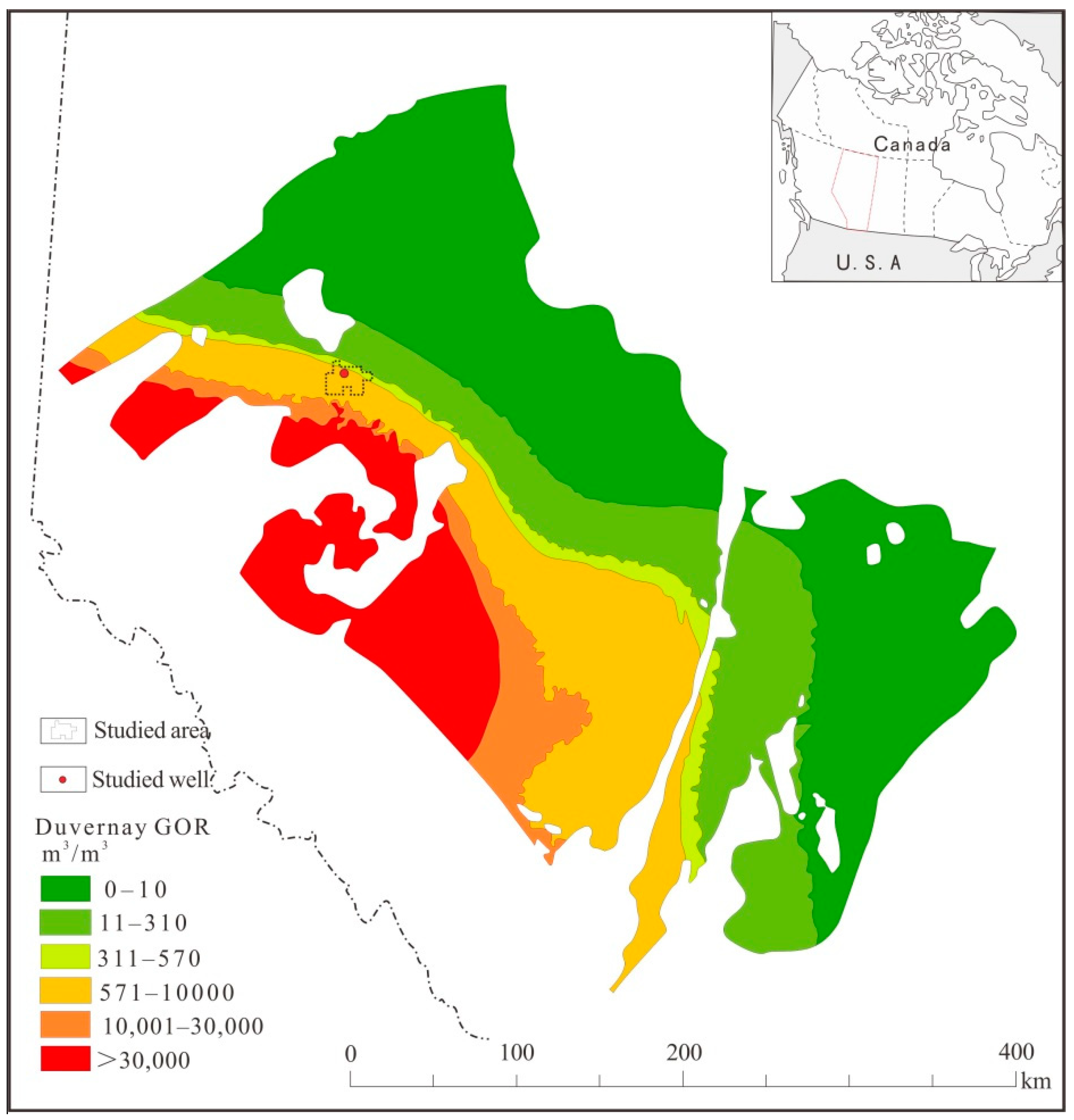
The studied reservoir is located at the volatile oil window of the Kaybob area. The reservoir is overpressured and the pressure coefficient is approximately 1.8. The reservoir thickness range is 30–45 m. Total organic carbon (TOC) of the reservoir ranges between 2% to 6%. The thermal maturity (Ro) range is 0.9–1.2%. The porosity averages around 5%, and matrix permeability is of hundreds nano Darcy [28]. The GOR of the volatile oil window in this region ranges from 2000 to 3500 scf/STB (stock tank barrel). Figure 1 shows the GOR of the Duvernay shale and the location of the subject well.

Figure 1. Gas-to-oil ratio (GOR) in the Duvernay shale and the location of the subject well (after Lyster et al. 2017) [23].

The Diagnostic Fracture Injection Test (DFIT) of the subject well in Duvernay shale indicates complex fractures mixed with hydraulic fractures and natural fractures near the wellbore. The density of natural fractures is 0.1 fracture per meter along the horizontal wellbore according to OBMI (Oil-Base Micro-Imager) image log interpretation. The strike of natural fractures is dominated by NW–SE, which is parallel with the trajectory of the horizontal well. The estimated formation pressure and permeability for the subject well are 63.84 MPa and 0.0028 mD, respectively.

3.2. Fluid Characterization

Eight pseudocomponents were assigned in this study: N₂, CO₂, CH₄, C₂H₆, C₃H₈, C₄, C₅–C₆, and C₇₊. The corresponding molar fractions were 0.0026, 0.0053, 0.5403, 0.1260, 0.0764, 0.0480, 0.0522, and 0.1492, respectively. We tune the Peng–Robinson equation of state (PR EOS) by the bulk fluid PVT data from laboratory reports such as Constant Composition Expansion (CCE) and Differential Liberation (DL) tests. The oil properties were determined for this well using the Peng–Robinson EOS and flash calculations under a reservoir temperature of 124 °C. Oil gravity was 45°API, gas/oil ratio was 4000 scf/STB, formation volume factor was 1.65 RB/STB, the bubble point pressure was 3492 psi, and the minimum miscible pressure (MMP) was 22.48 MPa. Detailed data for the PR EOS and the binary interaction parameters are listed in Table 1 and Table 2.

Table 1. Compositional data for the Duvernay volatile oil well.

Component	Molar Fraction	Critical Pressure [atm]	Critical Temperature [K]	Critical Volume [L/mol]	Molar Weight [g/gmol]	Acentric Factor	Parachor Coefficient
N2	0.0026	33.50	126.20	0.0895	28.01	0.0400	41.00
CO2	0.0053	72.80	304.20	0.0940	44.01	0.2250	78.00
CH4	0.5403	45.40	190.60	0.0990	16.04	0.0080	77.00
C2H6	0.1260	48.20	305.40	0.1480	30.07	0.0980	108.00
C3H8	0.0764	41.90	369.80	0.2030	44.10	0.1520	150.30
C4	0.0480	37.06	427.62	0.2058	23.81	0.2344	187.47
C5–C6	0.0522	33.00	507.00	0.1222	77.57	0.2500	237.58
C7+	0.1492	20.28	655.58	0.7073	157.30	0.4882	484.01

Table 2. Binary interaction parameters for the Duvernay volatile oil well.

Component	N2	CO2	CH4	C2H6	C3H8	C4	C5–C6	C7+
N2	0.0000	−0.0200	0.0310	0.0420	0.0910	0.0950	0.1100	0.1300
CO2	−0.0200	0.0000	0.1200	0.1100	0.1000	0.1200	0.1250	0.1400
CH4	0.0310	0.1200	0.0000	0.0040	0.0128	0.0133	0.0011	0.0906
C2H6	0.0420	0.1100	0.0040	0.0000	0.0025	0.0027	0.0009	0.0587
C3H8	0.0910	0.1000	0.0128	0.0025	0.0000	0.0000	0.0064	0.0379
C4	0.0950	0.1200	0.0133	0.0027	0.0000	0.0000	0.0068	0.0371
C5–C6	0.1100	0.1250	0.0011	0.0009	0.0064	0.0068	0.0000	0.0732
C7+	0.1300	0.1400	0.0906	0.0587	0.0379	0.0371	0.0732	0.0000

3.3. Numerical Modeling Set-Up with Complex Fractures

The subject well was hydraulically-fractured in 21 stages, with 3 clusters per stage along a lateral length of 1860 m. The hydraulic fracture pattern is assumed to be multiple bi-wing fractures with evenly fracture spacing, the number of fractures is 63. The initial pressure of this volatile oil reservoir is about 63.8 MPa. The primary production of the well consists of oil, gas, and water.

The model size is set based on the lateral length, well spacing and reservoir thickness of the subject well. The lateral length, well spacing and reservoir thickness are 1860 m, 300 m, and 45 m, respectively. In order to make sure that the model can fully cover the well and avoid boundary effect, we set the model size to 2600 m × 610 m × 45 m, which corresponds to length, width, and height, respectively. Since the spacing of hydraulic fractures is 30 m, to ensure that there are at least two sets of grid blocks among each hydraulic fractures, the grid size along the x-axis (length) is set to 10 m. We set the same grid size for the y-axis (width). The grid size for the vertical axis is set to 5 m, which we believe it is enough for running fracture models. Thus, the number of grid blocks is 260 × 61 × 9, and the grid cell dimension is 10 m × 10 m × 5 m.

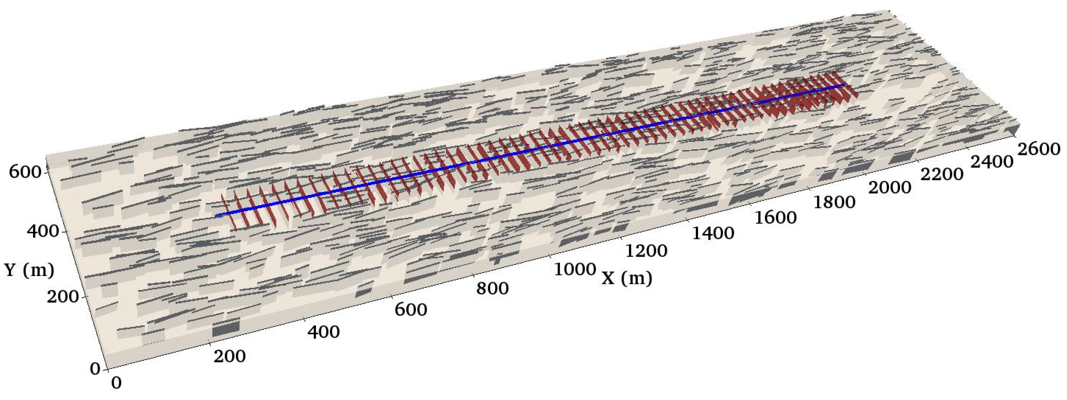
Both natural fractures and hydraulic fractures were considered in numerical modeling, and EDFM was performed to establish fracture models [29,30]. Based on the equivalent conductivity, the width of hydraulic fractures is set to 0.4 m and the permeability is 2.5 mD, that is, the conductivity of hydraulic fracture is 100 mD·cm. Considering the fracture density of the natural fractures, assuming that the density of natural fractures is 0.1/m, the permeability of the unstimulated area is 0.001 mD, and the permeability of the stimulated area is equal to the permeability of hydraulic fractures to 2.5 mD. According to core data from the subject well, the width of natural fractures is set to 0.004 m. Then, the conductivity of natural fracture in the unstimulated area is 0.0004 mD·cm. Figure 2 shows the numerical model with 63 hydraulic fractures (in red) and 1000 natural fractures (in grey).

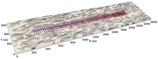
Figure 2. Numerical model with hydraulic fractures (in red) and natural fractures (in grey).

Considering the simulation time, the model mainly considers two scales of pores, nano-scale matrix systems, and micro-centimeter-scale fracture systems (including natural fractures and hydraulic fractures) [31,32]. By adjusting the critical properties of different components, two sets of EOS are set for different pore systems. The critical properties of the components corresponding to each pore radius were calculated according to Equation (4) to Equation (6). Table 3 lists the critical pressure and temperature of the eight pseudocomponents corresponding to the pore radius of 10 nm, 30 nm, 50 nm, 2000 nm and bulk phase. The base case of the pore radius for the matrix is set to 10 nm.

Table 3. Critical properties of the eight pseudocomponents corresponding to different pore radius in Duvernay volatile oil well.

Component	Bulk Phase		rp = 10 nm		rp = 30 nm		rp = 50 nm		rp = 2000 nm
	Pc [atm]	Tc [K]	Pc [atm]	Tc [K]	Pc [atm]	Tc [K]	Pc [atm]	Tc [K]	Pc [atm]	Tc [K]
N2	33.50	126.20	32.31	121.74	33.10	124.70	33.26	125.30	33.49	126.18
CO2	72.80	304.20	70.14	293.06	71.91	300.46	72.26	301.95	72.79	304.14
CH4	45.40	190.60	43.74	183.61	44.84	188.25	45.06	189.19	45.39	190.56
C2H6	48.20	305.40	46.18	292.58	47.52	301.09	47.79	302.81	48.19	305.34
C3H8	41.90	369.80	39.94	352.48	41.24	363.98	41.50	366.30	41.89	369.71
C4	37.06	427.62	35.16	405.75	36.42	420.26	36.67	423.19	37.05	427.51
C5–C6	33.00	507.00	31.15	478.51	32.38	497.40	32.62	501.23	32.99	506.86
C7+	20.28	655.58	18.83	608.59	19.79	639.70	19.99	646.03	20.28	655.34

Molecular diffusion can be described by Fick’s law, which can be used to describe the characteristics of pore-scale mass transfer and diffusion caused by concentration differences [33]. It has a certain impact on the effect of gas injection and shale oil production.

Molecular diffusion parameters can usually be obtained by fitting the results of laboratory experiments. The molecular diffusion characteristic value of the methane–propane system is about 2 × 10⁻⁴–10⁻³ cm²/s (70 °C, 10–20 MPa). Usually other mechanisms will also be considered in the molecular diffusion mechanism, so this parameter is usually larger than the actual value and is usually used as tuning parameters for calibrating numerical models. The gas diffusion coefficients are usually an order of magnitude larger than the oil diffusion coefficients. Hamdi et al. [6] used diffusion coefficients of 0.01 cm²/s [16] and 0.001 cm²/s for the light components in the gas and oil phases, respectively. In this paper, we took Hamdi’s assumption as reference, and set the diffusion coefficient of CH₄ as 0.01 cm²/s, then the diffusion coefficient of the other components were set according to their molecular weight. The molecular diffusion parameters of different components are shown in Table 4.

Table 4. Diffusion coefficients of different components.

Component	Diffusion Coefficient [cm2/s]
N2	0.008000
CO2	0.007692
CH4	0.01000
C2H6	0.007692
C3H8	0.003846
C4	0.001282
C5+	0.000256

It should be pointed out that the model we built is a single well model. Well spacing and well interference cannot be investigated using the model. This is mainly because we aim to discuss the geological and engineering control on huff and puff, however, a multiple well model could complicate the effect of these parameters.

3.4. History-Matching Parameters

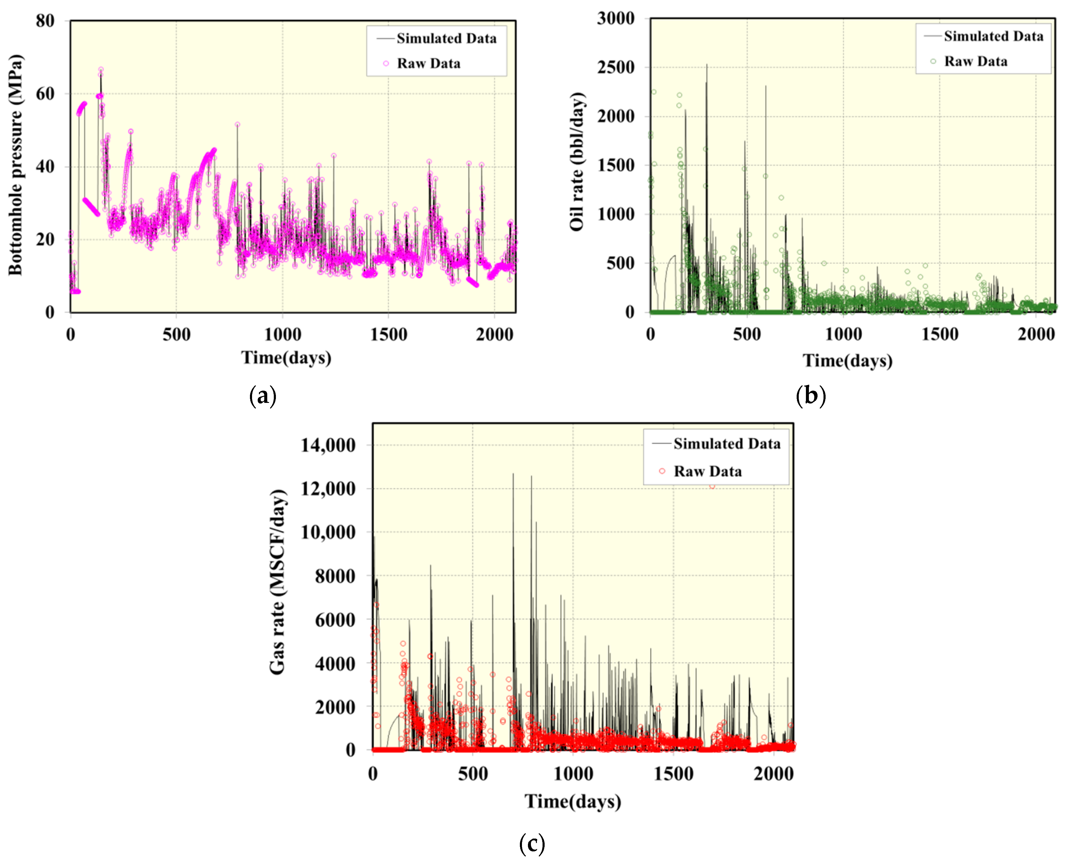
Based on the numerical model constructed in this paper, history matching was conducted. Although the production data is noisy, a good history match of oil rate was achieved as shown in Figure 3. The history matched parameters are listed in Table 5, which are the basic reservoir and fracture inputs for production simulations. We use EDFM to efficiently and easily handle hydraulic fractures in the model. The flowing bottom-hole pressure (BHP) was applied for the reservoir simulation constraint.

Figure 3. Comparison of well performance between raw data and model results: (a) Bottomhole Pressure; (b) Oil Rate; (c) Gas Rate.

Table 5. Basic reservoir and fracture properties used for history matching.

Parameters	Value	Unit
Model dimension	2600 × 610 × 45	m
Number of grid blocks	260 × 61 × 9	–
Grid cell dimension	10 × 10 × 5	m
Initial reservoir pressure	63.8	MPa
Reservoir temperature	255	°F
Reservoir depth	3450	m
Reservoir porosity	0.035	–
Matrix permeability	0.0002	mD
Matrix water saturation	0.17	–
Fracture height	26.52	m
Fracture half-length	60	m
Fracture conductivity	100	mD.cm
Fracture water saturation	0.49	–
Fracture width	0.4	m

4. Effect of Reservoir, Completion, and Depletion Parameters on Huff-n-Puff in Duvernay Shale

Oil recovery during gas huff-n-puff in shale reservoirs is a complex function of mass transfer (including miscibility, interfacial-tension, swelling, and molecular diffusion) and other controlling factors such as hydraulic fracturing and geological heterogeneities [3,6,21].

Based on the numerical model constructed and the history-matched parameters, we proposed a set of parameters that can represent hydraulic fracturing and geological heterogeneities. These parameters can be divided into three types: reservoir, hydraulic fracturing and primary depletion. Table 6 summarizes the type, name, unit, range and base case of the geological and engineering parameters for the simulation.

Table 6. Summary of geological and engineering parameters for the simulation.

Type	Parameter	Unit	Range	Base Case
Reservoir	Thickness of reservoir	m	15, 30, 45, 60, 75	45
	TOC		2%, 4%, 6%, 10%	4%
	Pore radius	nm	10, 30, 50, 2000	10
	Matrix permeability	mD	5∙10−5, 1∙10−4, 2∙10−4, 5∙10−4	2∙10−4
	Natural fracture density	NO. of fractures/m	None, 0.05, 0.1, 0.2, 0.5	0.1
	Natural fracture permeability	mD	0.0005, 0.001, 0.002, 0.005	0.001
Hydraulic fracturing	Half-length of hydraulic fractures	m	35, 60, 85	60
	Fracture conductivity	mD·cm	10, 100, 1000, 10,000	100
	Type of stimulated reservoir volume (SRV) region		A, B, C, D	C
	Magnification of permeability in SRV region		1, 2, 5, 8	2
Primary Depletion	Period of primary depletion	year	1, 3, 5, 7	5
	BHP of primary depletion	MPa	35, 40, 45, 50	45

To examine the effects of these parameters on gas huff-n-puff in Duvernay shale, 37 cases were simulated. We set fixed operational parameters for all the cases. The gas huff-n-puff process began after five years of primary depletion. We used rich gas as the injected gas, which is composed of 70% of CH₄, 20% of C₂H₆, and 10% of C₃–C₄. The injection rate is set to 3.5 MMscf/d and the cumulative gas injection is 176.5 MMscf. Then, the well is brought back on production after soaking for 30 days. We shut the well when the oil rate declined to the rate before the gas huff-n-puff process (the oil rate after 5 years of primary depletion). The period from the end of soaking to the shut-in date is defined as the duration of the first huff-n-puff cycle. Cumulative Oil Production for Primary Depletion, incremental oil recovery, and gas usage ratio was calculated for each case.

The incremental oil recovery equals to incremental oil production with huff-n-puff divided by OOIP of the subject well. The OOIP of the subject well is calculated under the condition of 300 m well spacing, 1860 m lateral length, and 45 m reservoir thickness. The calculated OOIP of the subject well is 2682 Mbbl. Gas usage ratio is defined as total volume of injected gas divided by total barrels of improved oil production by gas injection.

4.1. Effect of Reservoir Parameters

4.1.1. Reservoir Thickness

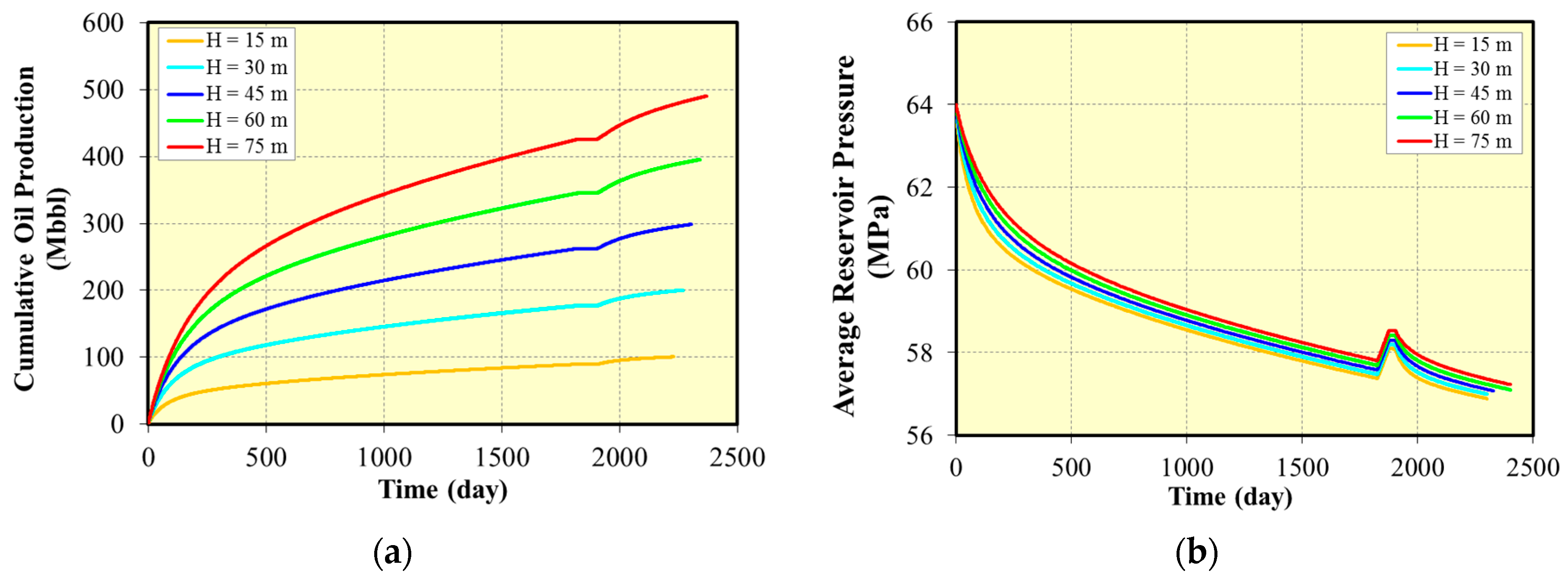
The simulated reservoir thickness includes 15 m, 30 m, 45 m, 60 m, and 75 m, and 45 m is set as the base case. Table 7 summarizes results for huff-n-puff with different reservoir thickness. What needs to be clarified is that we built five models for these five cases of reservoir thickness. The grid size of all of the cases is 10 m × 10 m × 5 m, and the difference among each case is the vertical number of grid blocks. In particular, we adjusted the cumulative volume of injected gas with respect to different reservoir thickness. The results of cumulative oil production, average reservoir pressure, incremental oil recovery, duration of the first huff-n-puff cycle and gas usage ratio were plotted in Figure 4 and Figure 5. As can be seen from these figures, thick reservoirs produced more oil during primary depletion, whereas the lowest incremental oil recovery and highest gas usage ratio were observed in the thickest reservoir. We also noticed the duration of the first huff-n-puff cycle increased with the increase of reservoir thickness. Even if the incremental oil recovery was lower in thicker reservoirs, a minimum thickness of 30 m was proposed for gas huff-n-puff due to the higher primary production in thicker reservoirs.

Table 7. Summary of results for huff-n-puff with different reservoir thickness.

Thickness of Reservoir (m)	15	30	45	60	75
Oil rate after 5 years primary depletion (bbl/d)	16.42	33.09	50.07	67.49	85.23
Cumulative oil production for primary depletion (Mbbl)	89.51	177.11	262.52	345.53	426.03
Cumulative volume of injected gas for first huff-n-puff cycle (MMscf)	58.83	117.67	176.50	235.33	294.17
Cumulative oil production with one huff-n-puff cycle (Mbbl)	95.26	188.31	278.62	366.17	451.01
Duration of the first huff-n-puff cycle (d)	325	365	400	435	465
Gas usage ratio for the first huff-n-puff cycle (Mscf/STB)	10.25	10.50	10.96	11.40	11.78
Incremental oil recovery for the first huff-n-puff cycle (%)	0.64	0.63	0.60	0.58	0.56

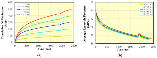
Figure 4. Effect of different reservoir thickness with one huff-n-puff cycle on oil production and reservoir pressure: (a) Cumulative oil production for different reservoir thickness; (b) Average reservoir pressure for different reservoir thickness.

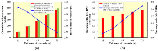
Figure 5. Correlation between reservoir thickness and huff-n-puff results: (a) Cumulative oil production and incremental oil recovery for different reservoir thickness; (b) Duration of the first huff-n-puff cycle and gas usage ratio for different reservoir thickness.

4.1.2. TOC

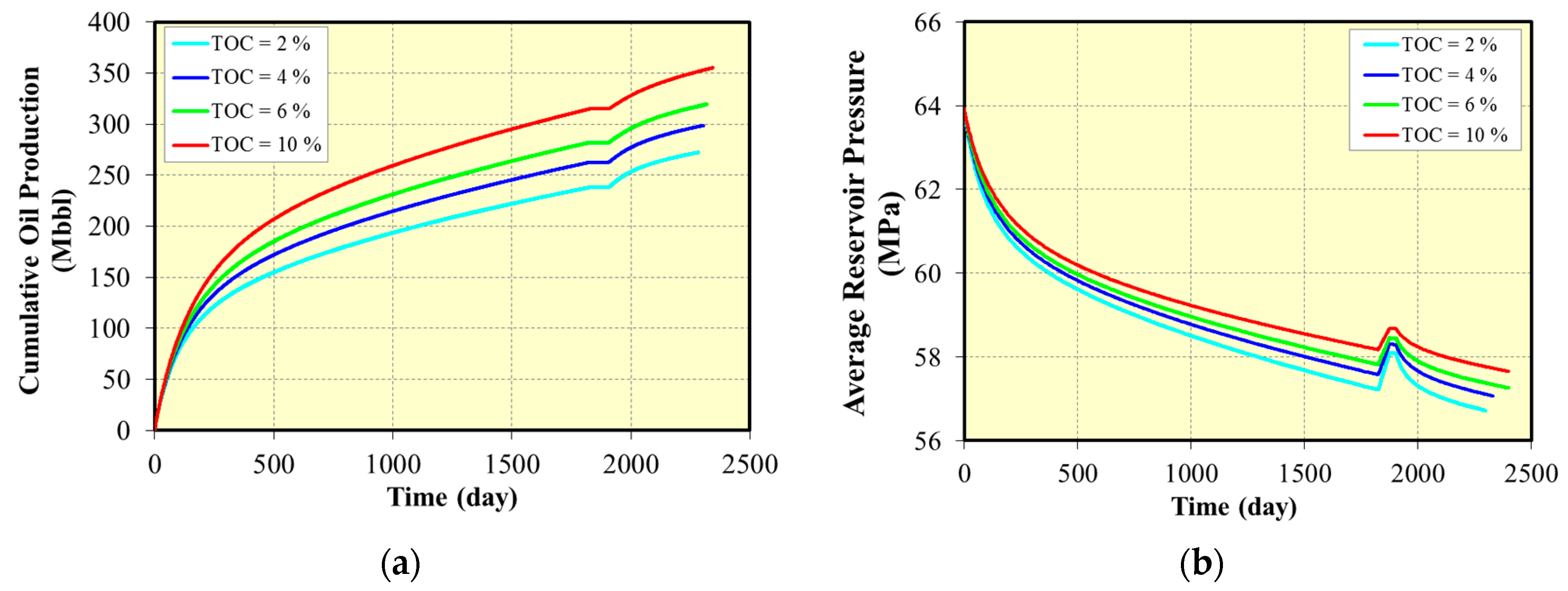
The effect of TOC was quantified by adsorbed gas content which increased with the increase of TOC. As shown in Table 8, TOC of 2%, 4%, 6%, and 10% were examined in this study. Figure 6 and Figure 7 indicate that cases with higher TOC shows higher cumulative oil production due to the desorption of the adsorbed gas. The incremental oil recovery shows a negative correlation with TOC, but the variance among different TOC is minor. Due to the desorption effect, the duration shows a positive correlation with TOC.

Table 8. Summary of results for huff-n-puff with different TOC.

TOC (%)	2	4	6	10
Oil rate after 5 years primary depletion (bbl/d)	46.61	50.07	52.77	57.36
Cumulative oil production for primary depletion (Mbbl)	255.65	282.55	303.71	340.01
Cumulative volume of injected gas for first huff-n-puff cycle (MMscf)	176.50	176.50	176.50	176.50
Cumulative oil production with one huff-n-puff cycle (Mbbl)	272.33	298.65	319.46	355.16
Duration of the first huff-n-puff cycle (d)	380	400	415	441
Gas usage ratio for the first huff-n-puff cycle (Mscf/STB)	10.58	10.96	11.21	11.65
Incremental oil recovery for the first huff-n-puff cycle (%)	0.62	0.60	0.59	0.56

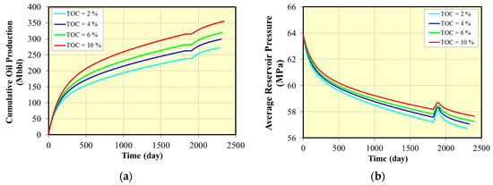
Figure 6. Effect of different TOC with one huff-n-puff cycle on oil production and reservoir pressure: (a) Cumulative oil production for different TOC; (b) Average reservoir pressure for different TOC.

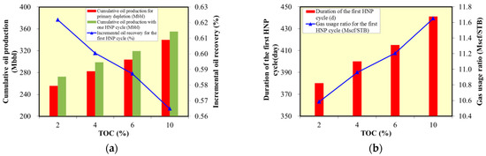
Figure 7. Correlation between TOC and huff-n-puff results: (a) Cumulative oil production and incremental oil recovery for different TOC; (b) Duration of the first huff-n-puff cycle and gas usage ratio for different TOC.

4.1.3. Pore Radius of Shale Matrix

The nanopore confinement in shale reservoirs would lead to an increase in capillary pressure, which has a significant impact on the phase characteristics, critical properties, and physical properties of the fluid [34]. In numerical simulation, the effect of nanopore confinement can be calculated by modifying the equation of state.

The pores in Duvernay shale are mainly organic pores and the pore throats are of nano-scale, their radius is mainly 2–50 nm, and the radius of the organic pores is about 10 nm. We set the base case of pore radius to 10 nm. Additionally, the pore radius of 30 nm, 50 nm and 2000 nm were examined for gas huff-n-puff. It can be seen from Table 9, Figure 8 and Figure 9 that the smaller the pore radius, the higher the cumulative oil production, but the difference is slight. This is due to the low density and low viscosity of the oil phase under the low pore radius, which is conducive to oil phase flow. The results imply that the effect of pore radius on gas huff-n-puff was marginal.

Table 9. Summary of results for huff-n-puff with different pore radius of shale matrix.

Pore Radius of Shale Matrix (nm)	10	30	50	2000
Oil rate after 5 years primary depletion (bbl/d)	50.07	49.06	48.87	48.62
Cumulative oil production for primary depletion (Mbbl)	282.55	275.66	274.05	272.03
Cumulative volume of injected gas for first huff-n-puff cycle (MMscf)	176.50	176.50	176.50	176.50
Cumulative oil production with one huff-n-puff cycle (Mbbl)	298.65	291.69	290.25	288.39
Duration of the first huff-n-puff cycle (d)	400	400	395	395
Gas usage ratio for the first huff-n-puff cycle (Mscf/STB)	10.96	11.01	10.89	10.79
Incremental oil recovery for the first huff-n-puff cycle (%)	0.60	0.60	0.60	0.61

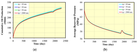
Figure 8. Effect of different pore radius of shale matrix with one huff-n-puff cycle on oil production and reservoir pressure: (a) Cumulative oil production for different pore radius of shale matrix; (b) Average reservoir pressure for different pore radius of shale matrix.

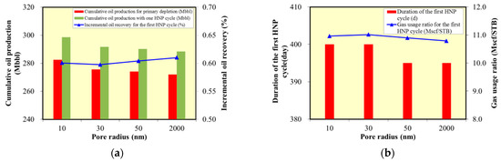
Figure 9. Correlation between pore radius of shale matrix and huff-n-puff results: (a) Cumulative oil production and incremental oil recovery for different pore radius of shale matrix; (b) Duration of the first huff-n-puff cycle and gas usage ratio for different pore radius of shale matrix.

4.1.4. Matrix Permeability

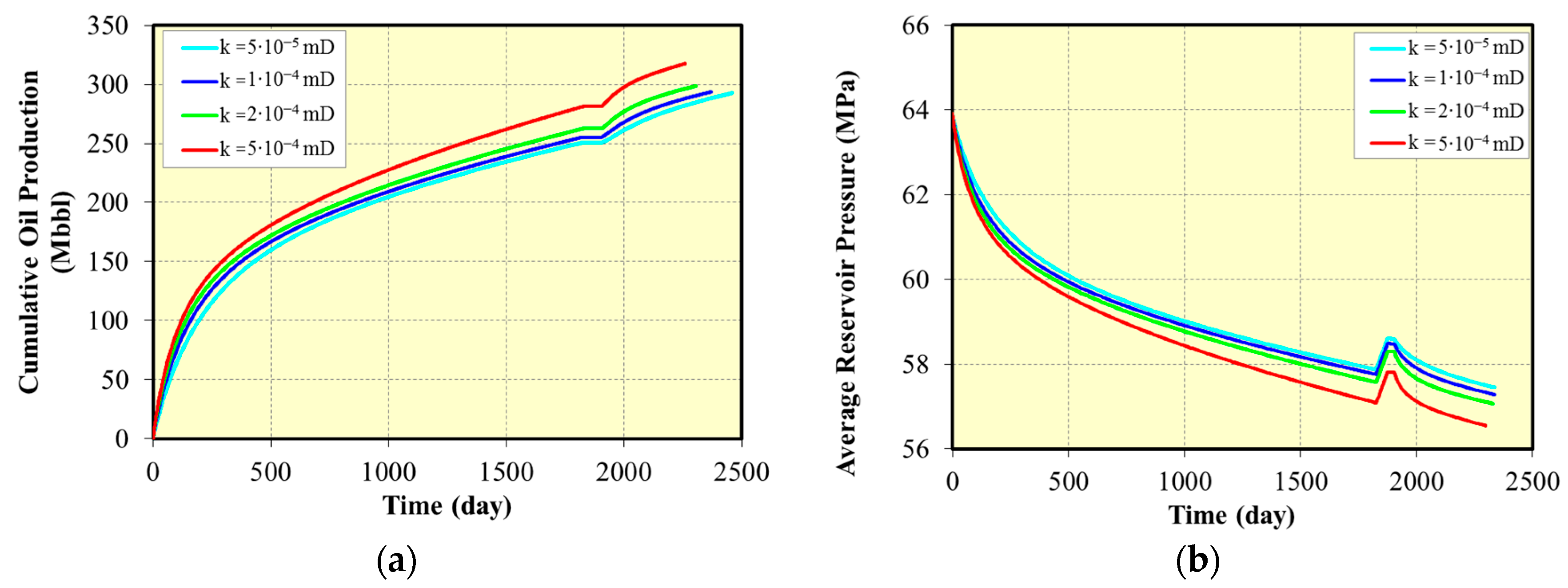
Four cases of different matrix permeability were simulated and results were shown in Table 10, Figure 10 and Figure 11. Lower matrix permeability could result in lower cumulative oil production and higher average reservoir pressure. Higher matrix permeability is beneficial for incremental oil recovery and gas usage ratio, but the difference is minor. However, higher matrix permeability could shorten the duration of the first huff-n-puff cycle due to its high flowing rate in the reservoir. The recommended matrix permeability for huff-n-puff is ≥5∙10⁻⁵ mD. The higher permeability is conducive to injecting gas to displace the fluid in the matrix.

Table 10. Summary of results for huff-n-puff with different matrix permeability.

Matrix Permeability (mD)	5∙10−5	1∙10−4	2∙10−4	5∙10−4
Oil rate after 5 years primary depletion (bbl/d)	47.36	48.06	50.07	56.30
Cumulative oil production for primary depletion (Mbbl)	250.78	255.36	262.52	281.21
Cumulative volume of injected gas for first huff-n-puff cycle (MMscf)	176.50	176.50	176.50	176.50
Duration of the first huff-n-puff cycle (d)	555	465	400	355
Cumulative oil production with one huff-n-puff cycle (Mbbl)	292.68	293.62	298.65	317.57
Gas usage ratio for the first huff-n-puff cycle (Mscf/STB)	11.31	11.09	10.96	10.78
Incremental oil recovery for the first huff-n-puff cycle (%)	0.58	0.59	0.60	0.61

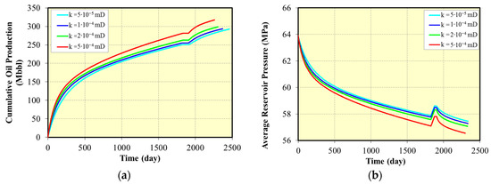
Figure 10. Effect of different matrix permeability with one huff-n-puff cycle on oil production and reservoir pressure: (a) Cumulative oil production for different matrix permeability; (b) Average reservoir pressure for different matrix permeability.

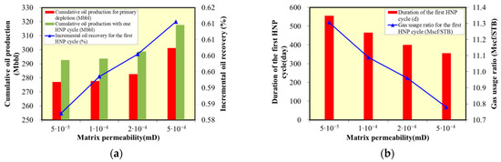
Figure 11. Correlation between matrix permeability and huff-n-puff results: (a) Cumulative oil production and incremental oil recovery for different matrix permeability; (b) Duration of the first huff-n-puff cycle and gas usage ratio for different matrix permeability.

4.1.5. Natural Fracture Density

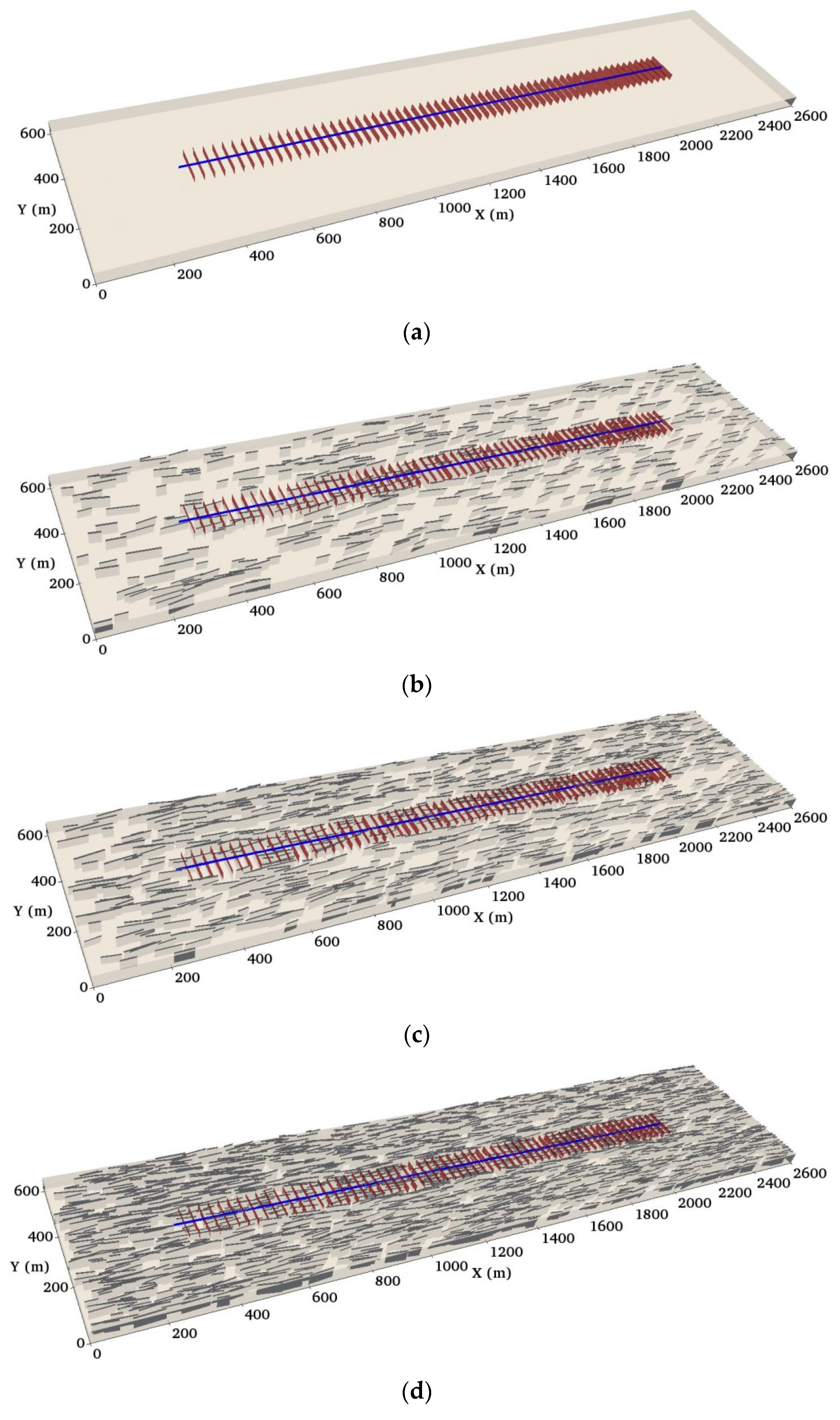
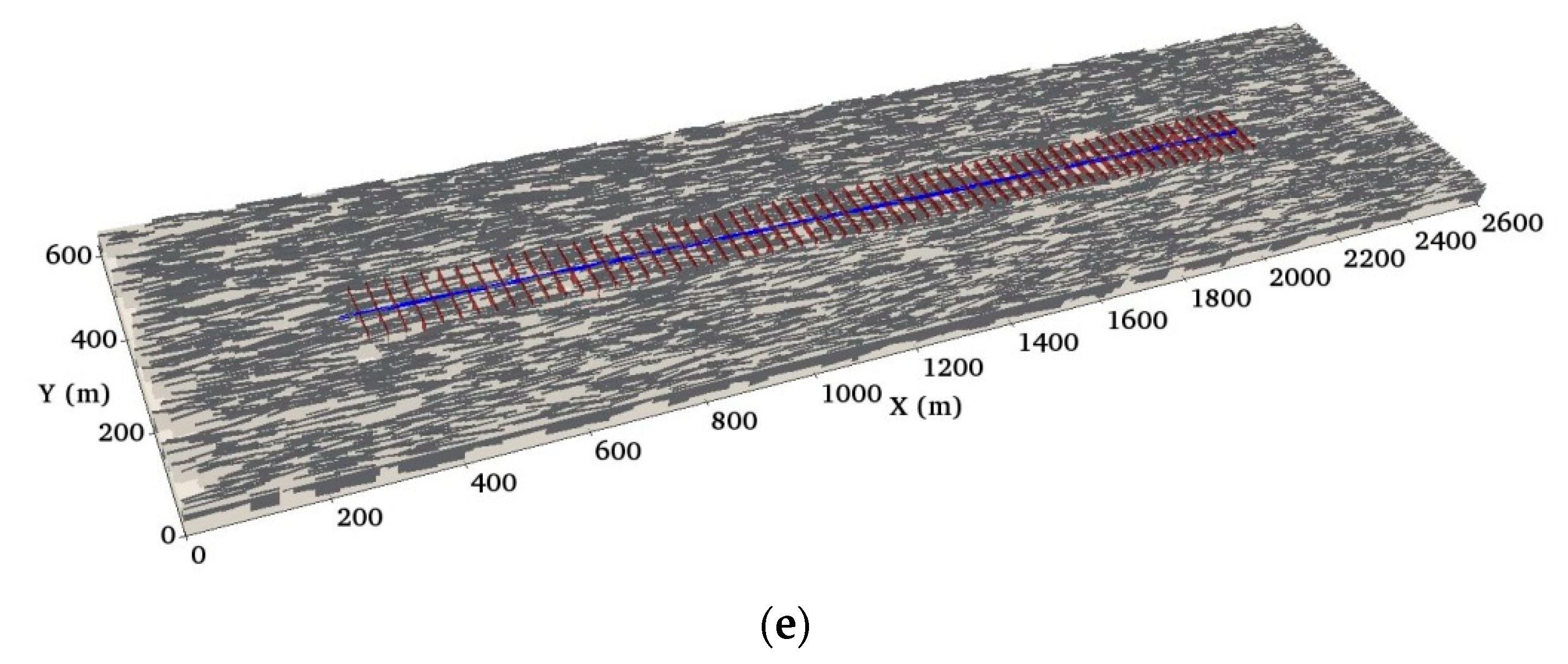
The effect of gas huff-n-puff under different natural fracture densities was analyzed. Five scenarios are considered. Figure 12 shows the numerical models for different scenarios. The results are shown in Table 11, and Figure 13 and Figure 14. It can be seen from the figures:

Figure 12. Numerical model with complex fractures: (a) without natural fractures; (b) 0.05 natural fracture/m; (c) 0.1 natural fracture/m; (d) 0.2 natural fracture/m; (e) 0.5 natural fracture/m. Blue line indicates the wellbore. Red and grey pieces represent hydraulic fractures and natural fractures respectively.

Table 11. Summary of results for huff-n-puff with different natural fracture density.

Natural Fracture Density (NO. of Fractures/m)	Without	0.05	0.1	0.2	0.5
Oil rate after 5 years primary depletion (bbl/d)	21.64	50.76	50.07	49.82	49.63
Cumulative oil production for primary depletion (Mbbl)	177.20	283.82	282.55	283.39	283.03
Cumulative volume of injected gas for first huff-n-puff cycle (MMscf)	176.50	176.50	176.50	176.50	176.50
Cumulative oil production with one huff-n-puff cycle (Mbbl)	196.45	298.82	298.65	302.52	306.42
Duration of the first huff-n-puff cycle (d)	765	445	400	420	425
Gas usage ratio for the first huff-n-puff cycle (Mscf/STB)	9.17	11.76	10.96	9.23	7.55
Incremental oil recovery for the first huff-n-puff cycle (%)	0.72	0.56	0.60	0.71	0.87

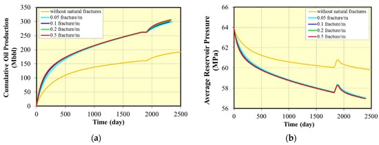
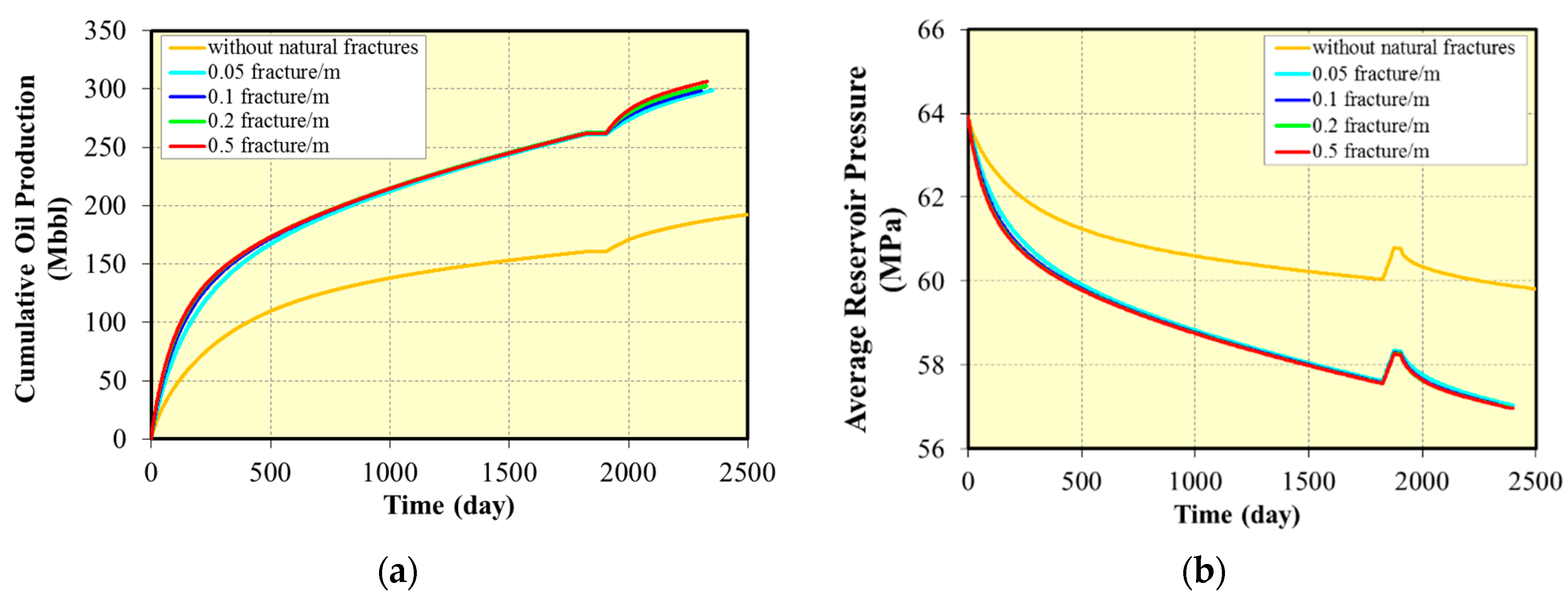
Figure 13. Effect of different natural fracture densities with one huff-n-puff cycle on oil production and reservoir pressure: (a) Cumulative oil production for different natural fracture densities; (b) Average reservoir pressure for different natural fracture densities.

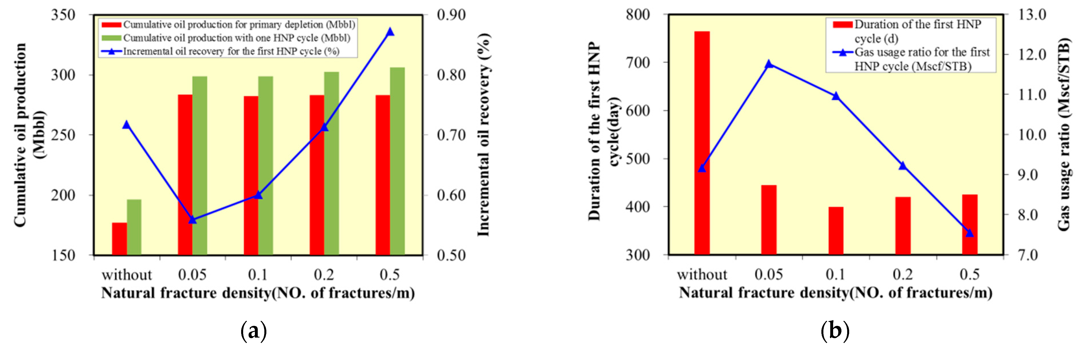
Figure 14. Correlation between natural fracture density and huff-n-puff results: (a) Cumulative oil production and incremental oil recovery for different natural fracture densities; (b) Duration of the first huff-n-puff cycle and gas usage ratio for different natural fracture densities.

The existence of natural fractures has a greater impact on the cumulative oil production for primary depletion which is 1.7 times compared with that without natural fractures.

When natural fractures are not considered, the oil rate after gas injection is low, but the duration of the first huff-n-puff cycle is much longer, which leads to a higher incremental oil recovery. When natural fractures exist, the density of natural fractures has a minor effect on the cumulative oil production for primary depletion. This is mainly due to the ultralow conductivity of natural fractures. According to core data from the subject well, the conductivity of natural fracture is 0.0004 mD·cm which is ultralow compared with that of hydraulic fractures (100 mD·cm). The simulation results indicate reducing fracture conductivity will significantly lowering primary depletion. The ultralow conductivity of natural fractures could result in the low impact of natural fracture density on primary depletion. Furthermore, the orientation of natural fractures is parallel to the horizontal well, so the hydraulic fractures can only connect limited natural fractures.

However, the incremental oil recovery increased significantly with the increase of natural fracture density. This can be attributed to a larger amount of injected gas available to contact the matrix area and extract hydrocarbons through natural fractures. The development of natural fractures is a favorable condition for gas huff-n-puff.

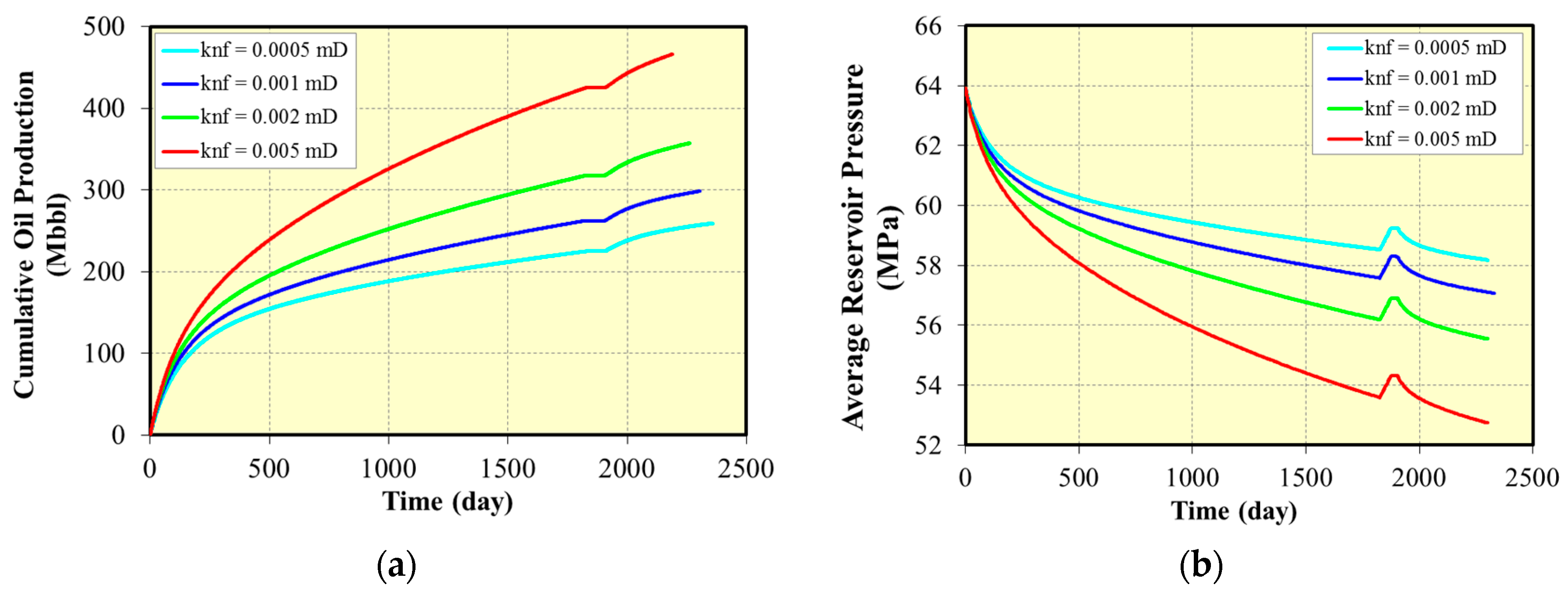
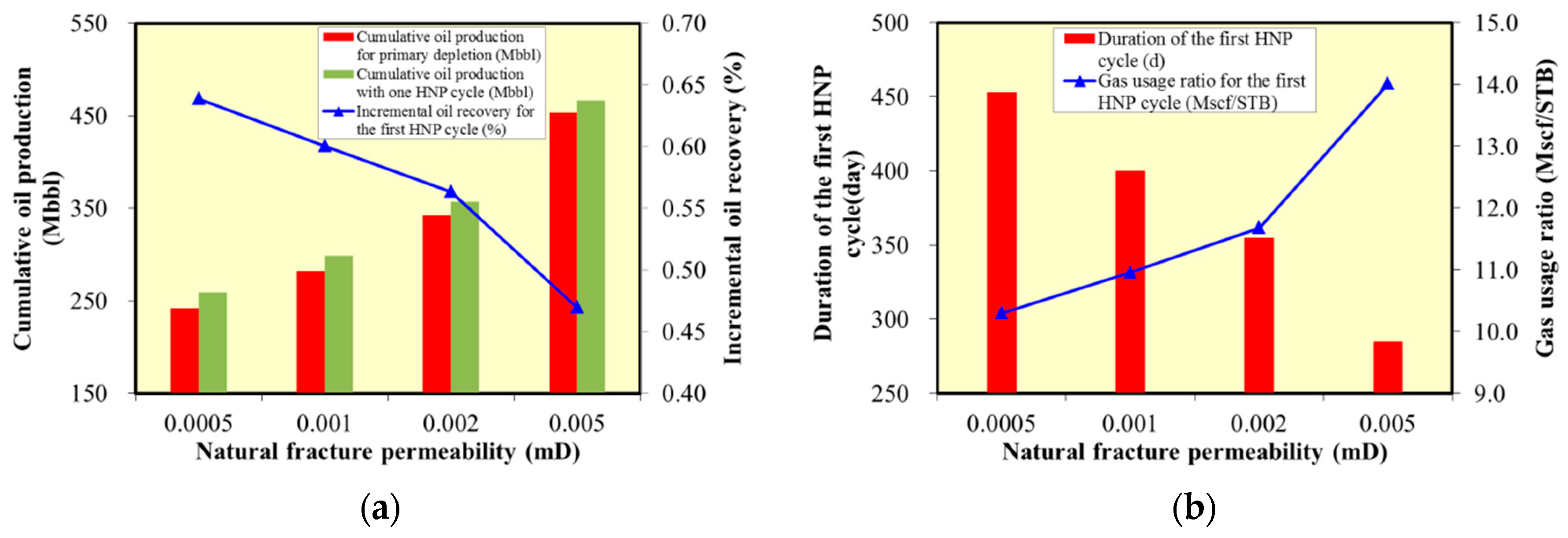
4.1.6. Natural Fracture Permeability

The effect of gas huff-n-puff under different natural fracture permeability was analyzed, and the results are shown in Table 12, and Figure 15 and Figure 16. It can be seen from the figures:

Table 12. Summary of results for huff-n-puff with different natural fracture permeability.

Natural Fracture Permeability (mD)	0.0005	0.001	0.002	0.005
Oil rate after 5 years primary depletion (bbl/d)	37.99	50.07	68.62	100.64
Cumulative oil production for primary depletion (Mbbl)	242.13	282.55	342.14	453.72
Cumulative volume of injected gas for first huff-n-puff cycle (MMscf)	176.50	176.50	176.50	176.50
Cumulative oil production with one huff-n-puff cycle (Mbbl)	259.27	298.65	357.25	466.32
Duration of the first huff-n-puff cycle (d)	453	400	355	285
Gas usage ratio for the first huff-n-puff cycle (Mscf/STB)	10.30	10.96	11.68	14.01
Incremental oil recovery for the first huff-n-puff cycle (%)	0.64	0.60	0.56	0.47

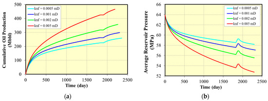
Figure 15. Effect of different natural fracture permeability with one huff-n-puff cycle on oil production and reservoir pressure: (a) Cumulative oil production for different natural fracture permeability; (b) Average reservoir pressure for different natural fracture permeability.

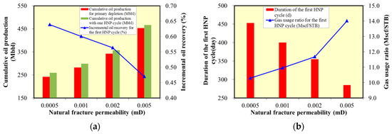
Figure 16. Correlation between natural fracture permeability and huff-n-puff results: (a) Cumulative oil production and incremental oil recovery for different natural fracture permeability; (b) Duration of the first huff-n-puff cycle and gas usage ratio for different natural fracture permeability.

Natural fracture permeability shows a distinct positive correlation with cumulative oil production, and high oil rate can be achieved with high natural fracture permeability.

The incremental oil recovery decreases with the increase of natural fracture permeability. This is attributed to the high oil recovery for primary depletion and the oil abundance near wellbore has been reduced by primary depletion. Meanwhile, natural fractures improve the pressure drop near wellbore, which makes it difficult to form a high-pressure zone near the wellbore and leads to a shorter duration of the gas huff-n-puff cycle. Increasing the total volume of injected gas could improve the effect of gas huff-n-puff and yield more additional oil.

4.2. Effect of Hydraulic Fracturing Parameters

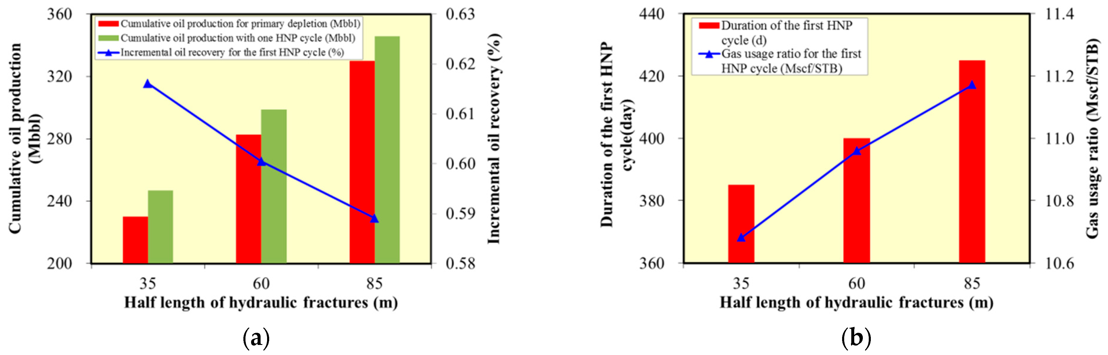
4.2.1. Half-Length of Hydraulic Fractures

Fracture half-length of 35 m, 60 m, and 85 m were simulated to examine its effect on gas huff-n-puff. The results are shown in Table 13, and Figure 17 and Figure 18. It can be seen from the figures:

Table 13. Summary of results for huff-n-puff with different half-length of hydraulic fractures.

Half-Length of Hydraulic Fractures (m)	35	60	85
Oil rate after 5 years primary depletion (bbl/d)	48.12	50.07	52.08
Cumulative oil production for primary depletion (Mbbl)	230.20	282.55	330.03
Cumulative volume of injected gas for first huff-n-puff cycle (MMscf)	176.50	176.50	176.50
Cumulative oil production with one huff-n-puff cycle (Mbbl)	246.72	298.65	345.83
Duration of the first huff-n-puff cycle (d)	385	400	425
Gas usage ratio for the first huff-n-puff cycle (Mscf/STB)	10.68	10.96	11.17
Incremental oil recovery for the first huff-n-puff cycle (%)	0.62	0.60	0.59

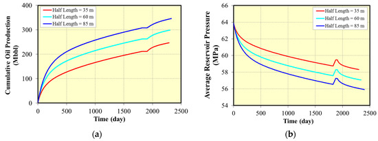
Figure 17. Effect of different half-length of hydraulic fractures with one huff-n-puff cycle on oil production and reservoir pressure: (a) Cumulative oil production for different half-length of hydraulic fractures; (b) Average reservoir pressure for different half-length of hydraulic fractures.

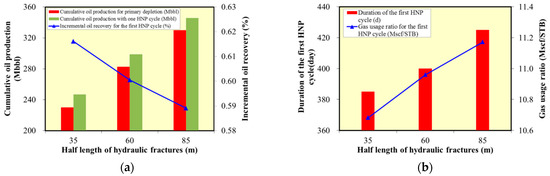
Figure 18. The correlation between half-length of hydraulic fractures and huff-n-puff results: (a) Cumulative oil production and incremental oil recovery for different half-length of hydraulic fractures; (b) Duration of the first huff-n-puff cycle and gas usage ratio for different half-length of hydraulic fractures.

Long fracture half-length has a significant contribution in shale reservoirs by increasing oil production during primary depletion. When the same volume of gas was injected, fracturing could weaken the effect of gas injection, and with the increase of fracture half-length, the incremental oil recovery could be decreased. This is because the injected gas needs to seep along the long fractures to the far well area, reducing the gas injection effect. Compared with the long fractures, if there are micro-fractures in the near well area, the effect of gas huff-n-puff is better.

The duration of the gas huff-n-puff cycle increases with the increase of fracture half-length. For long fracture half-length, the total volume of injected gas should be increased to improve the effect of gas huff-n-puff.

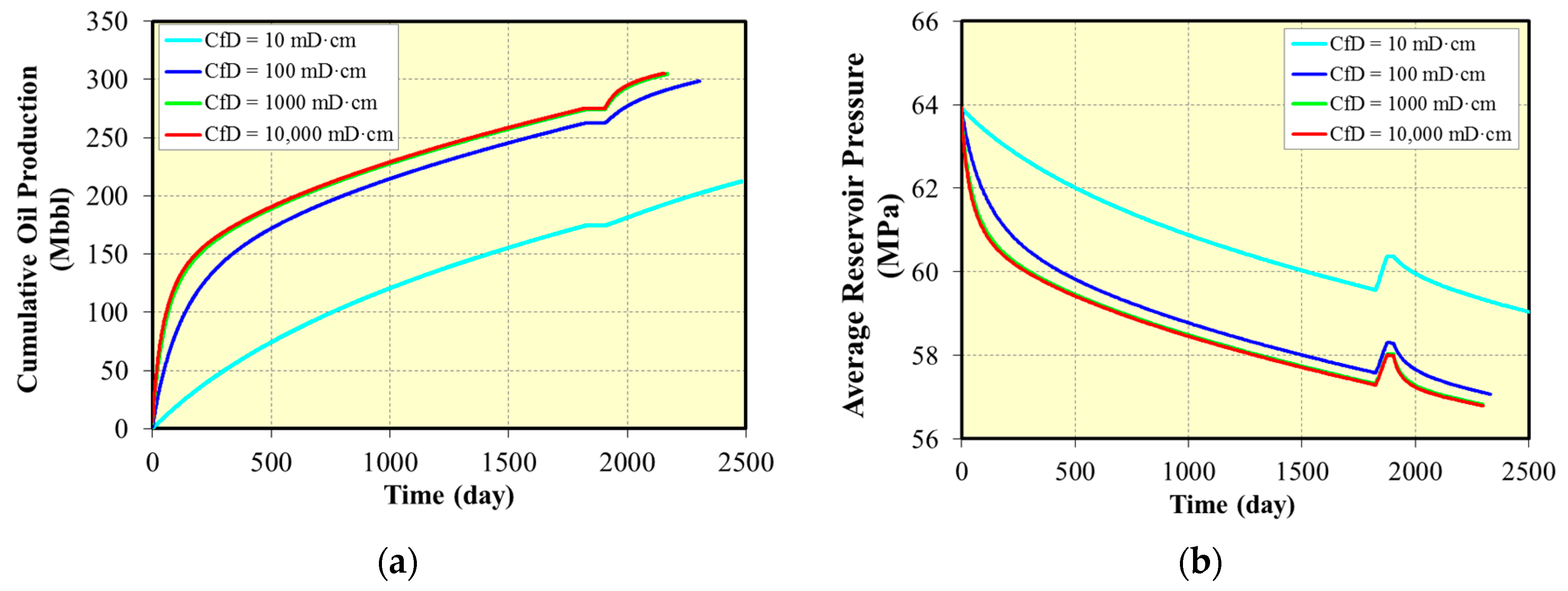
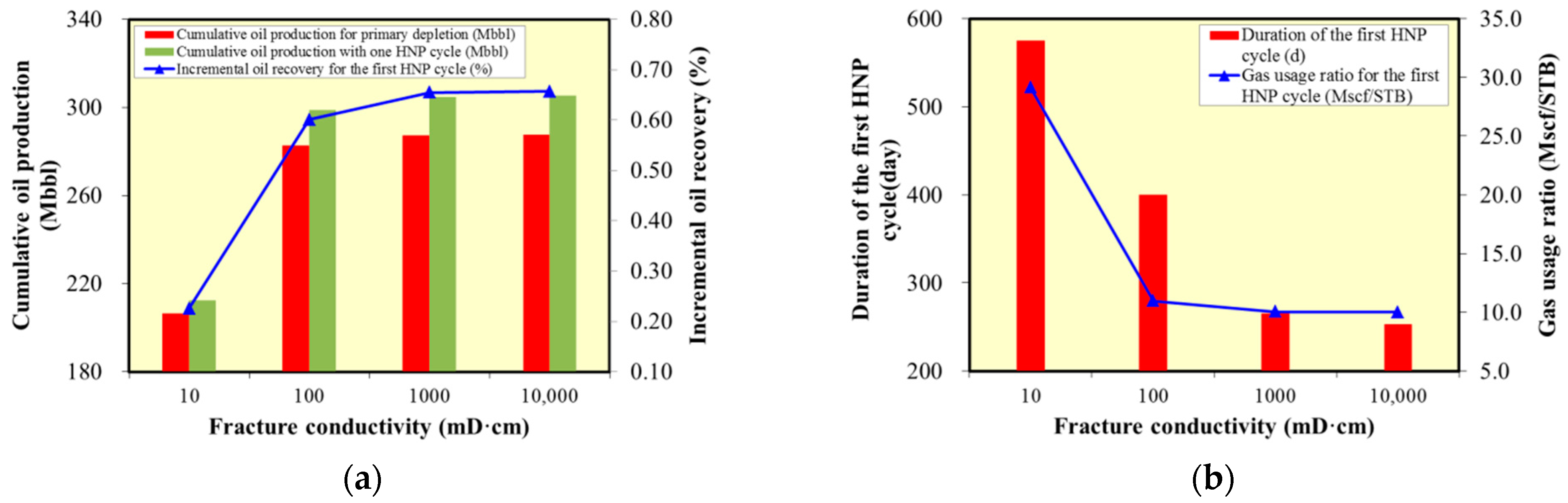
4.2.2. Fracture Conductivity

“System leakage” is a very practical and interesting topic for huff and puff. Fracture conductivity is an indicator of “leakage” or sealing capability. We analyzed the effect of gas huff-n-puff under different hydraulic fracture conductivity, results are shown in Table 14, and Figure 19 and Figure 20. It can be seen from the results that with the increase of fracture conductivity, the cumulative oil production for primary depletion and the incremental oil recovery increase, but the increase gradually flattens. When the fracture conductivity reaches 1000 mD·cm, there is a slight increase in cumulative oil production and oil recovery. So, it can be inferred that there is a limitation of conductivity. However, we believe the sealing capability of the reservoir more likely depends on the extension of hydraulic fractures and natural fractures instead of conductivity.

Table 14. Summary of results for huff-n-puff with different fracture conductivity.

Fracture Conductivity (mD·cm)	10	100	1000	10,000
Oil rate after 5 years primary depletion (bbl/d)	55.35	50.07	49.19	49.00
Cumulative oil production for primary depletion (Mbbl)	206.33	282.55	287.19	287.73
Cumulative volume of injected gas for first huff-n-puff cycle (MMscf)	176.50	176.50	176.50	176.50
Cumulative oil production with one huff-n-puff cycle (Mbbl)	212.38	298.65	304.75	305.35
Duration of the first huff-n-puff cycle (d)	575	400	265	253
Gas usage ratio for the first huff-n-puff cycle (Mscf/STB)	29.15	10.96	10.05	10.02
Incremental oil recovery for the first huff-n-puff cycle (%)	0.23	0.60	0.65	0.66

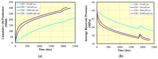
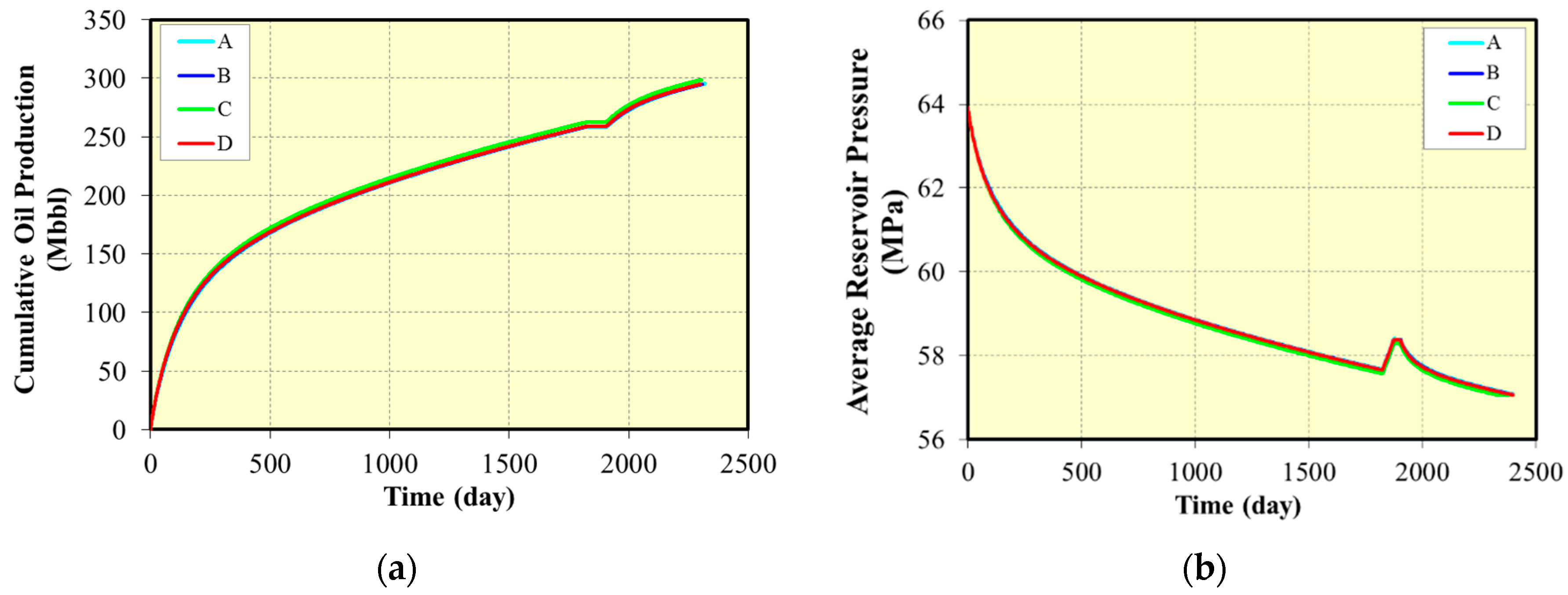
Figure 19. Effect of different fracture conductivity with one huff-n-puff cycle on oil production and reservoir pressure: (a) Cumulative oil production for different fracture conductivity; (b) Average reservoir pressure for different fracture conductivity.

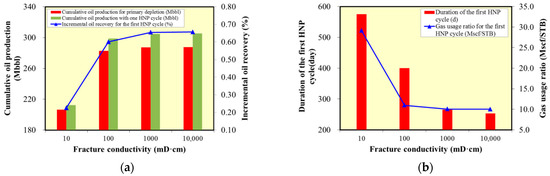
Figure 20. Correlation between fracture conductivity and huff-n-puff results: (a) Cumulative oil production and incremental oil recovery for different fracture conductivity; (b) Duration of the first huff-n-puff cycle and gas usage ratio for different fracture conductivity.

Wells with higher fracture conductivity is preferable for gas huff-n-puff. Fractures with high conductivity are conducive to gas injection into the formation to interact with crude oil. The recommended conductivity is greater than 100 mD·cm.

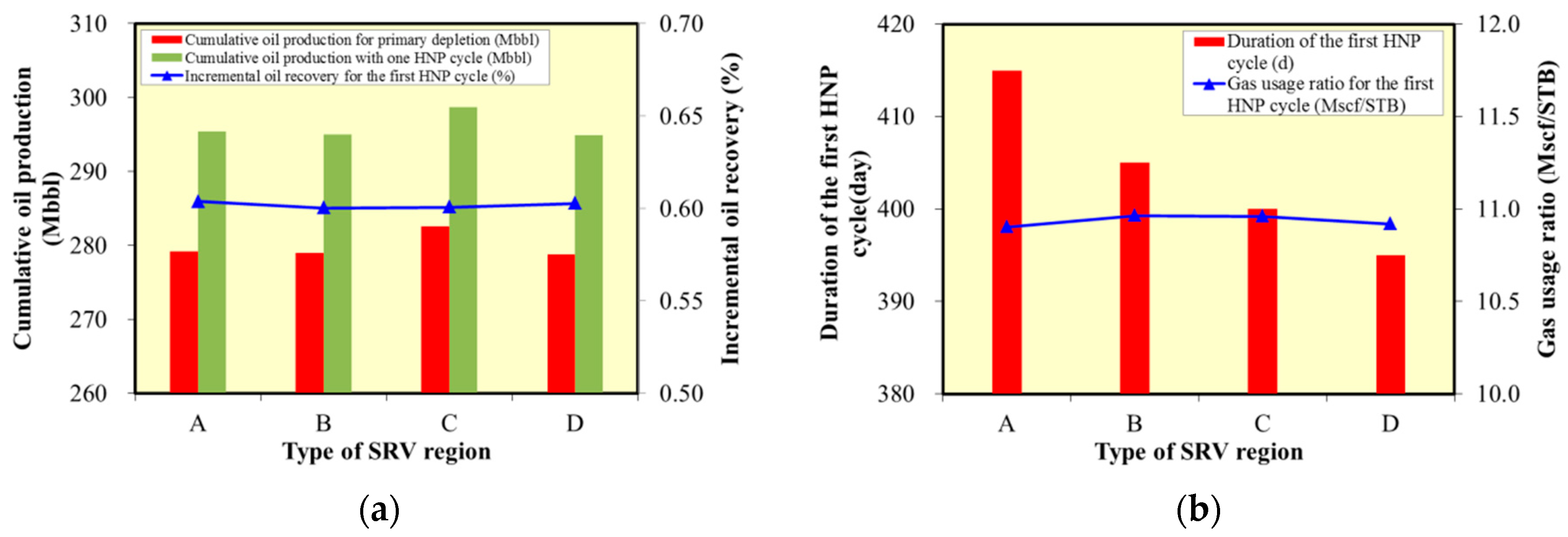
4.2.3. Type of SRV Region

The SRV region is defined by modification of permeability in these grid cells. We multiply the primary permeability of matrix and fractures by a number of times to represent the effect of stimulation. Considering the stimulated volume around the main hydraulic fractures, we assume four types of SRV region to represent no stimulation around main hydraulic fractures (Figure 21A), stimulation within 10 m of the single wing (Figure 21B), stimulation within 10 m of the bi-wing (Figure 21C), and stimulation within 20 m of the single wing (Figure 21D), respectively. The effect of the types of SRV region on gas huff-n-puff was analyzed. The results are summarized in Table 15, and Figure 22 and Figure 23, it can be seen from the figures that the types of SRV region show a very slight effect on gas huff-n-puff.

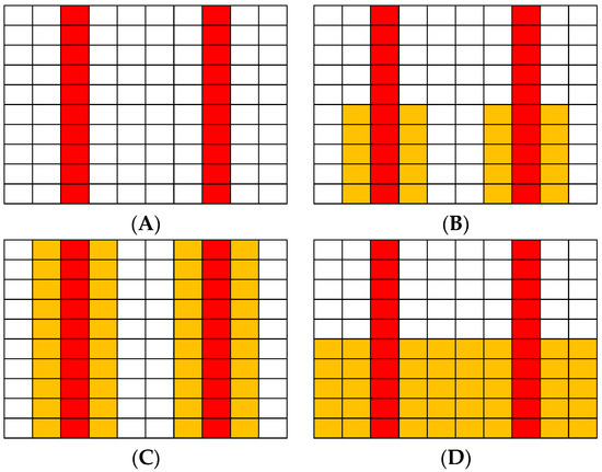
Figure 21. Four types of SRV region: (A) No stimulation around main hydraulic fractures; (B) Stimulation within 10 m of the single wing; (C) Stimulation within 10 m of the bi-wing; (D) Stimulation within 20 m of the single wing. The red grid indicates hydraulic fractures. The orange grid represents the SRV region. The white grid denotes matrix.

Table 15. Summary of results for huff-n-puff with different types of SRV region.

Type of SRV Region	A	B	C	D
Oil rate after 5 years primary depletion (bbl/d)	50.01	50.01	50.07	50.01
Cumulative oil production for primary depletion (Mbbl)	279.19	278.92	282.55	278.75
Cumulative volume of injected gas for first huff-n-puff cycle (MMscf)	176.50	176.50	176.50	176.50
Cumulative oil production with one huff-n-puff cycle (Mbbl)	295.37	295.02	298.65	294.91
Duration of the first huff-n-puff cycle (d)	415	405	400	395
Gas usage ratio for the first huff-n-puff cycle (Mscf/STB)	10.90	10.97	10.96	10.92
Incremental oil recovery for the first huff-n-puff cycle (%)	0.60	0.60	0.60	0.60

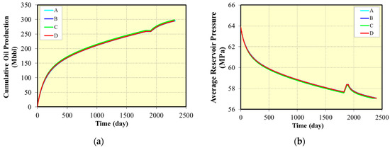
Figure 22. Effect of different types of SRV region with one huff-n-puff cycle on oil production and reservoir pressure: (a) Cumulative oil production for different types of SRV region; (b) Average reservoir pressure for different types of SRV region.

Figure 23. The correlation between types of SRV region and huff-n-puff results: (a) Cumulative oil production and incremental oil recovery for different types of SRV region; (b) Duration of the first huff-n-puff cycle and gas usage ratio for different types of SRV region.

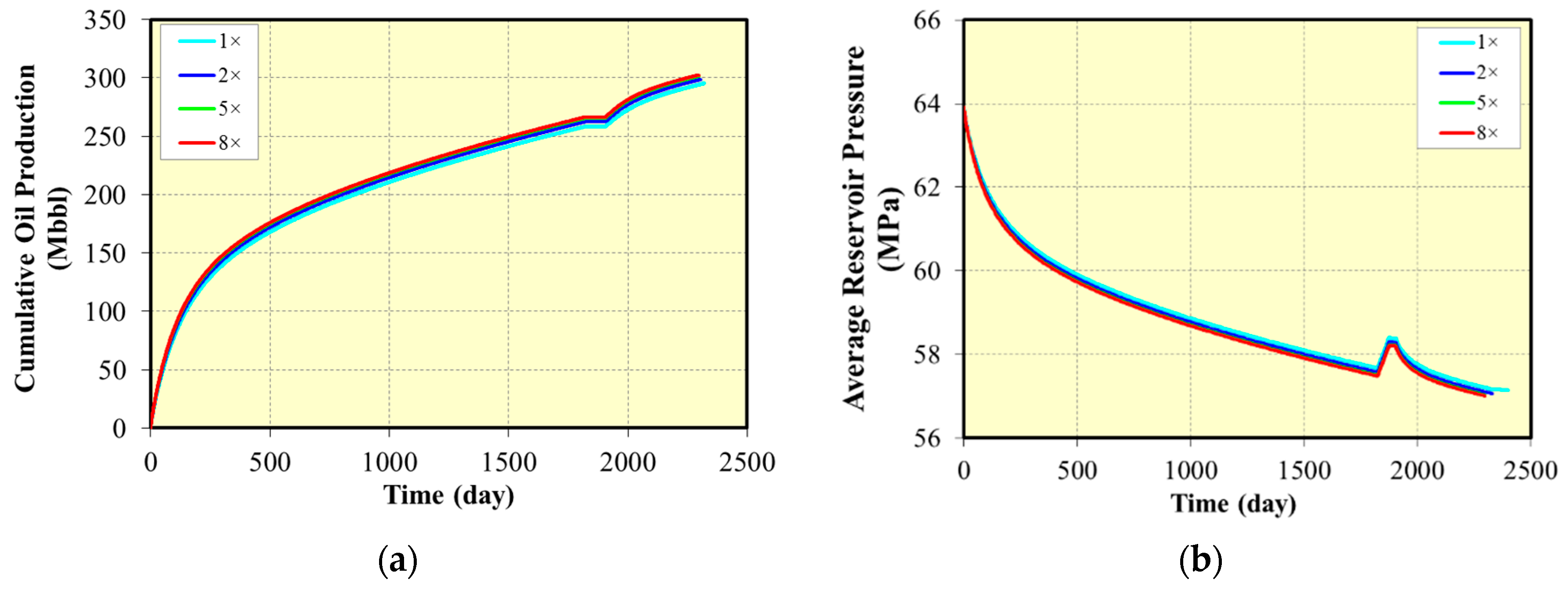
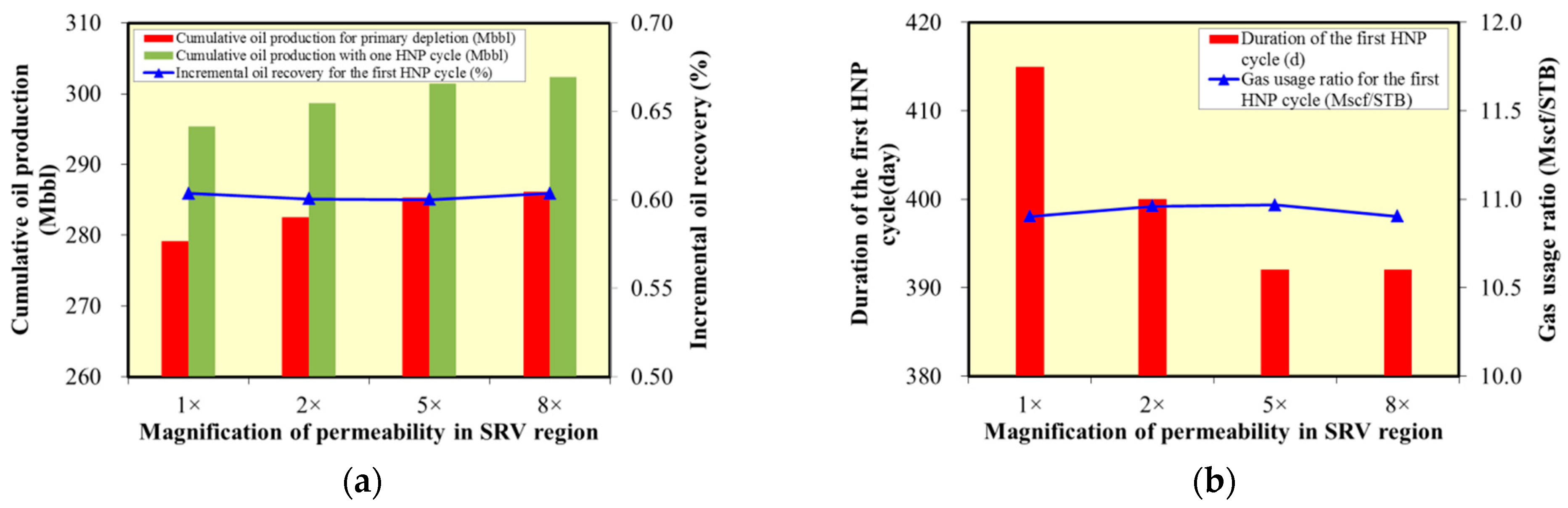
4.2.4. Magnification of Permeability in SRV Region

To further examine the effect of hydraulic fracturing, we set different permeability magnifications in the SRV region, which are 1×, 2×, 5×, and 8×. We increased the permeability in the SRV region (Orange grids in Figure 21C) by one time, two times, five times, and eight times. The results are summarized in Table 16, and Figure 24 and Figure 25, from the figures it can be seen:

Table 16. Summary of results for huff-n-puff with different permeability magnifications in the SRV region.

Magnification of Permeability in SRV Region	1×	2×	5×	8×
Oil rate after 5 years primary depletion (bbl/d)	50.01	50.07	50.19	50.07
Cumulative oil production for primary depletion (Mbbl)	279.19	282.55	285.31	286.18
Cumulative volume of injected gas for first huff-n-puff cycle (MMscf)	176.50	176.50	176.50	176.50
Cumulative oil production with one huff-n-puff cycle (Mbbl)	295.37	298.65	301.40	302.37
Duration of the first huff-n-puff cycle (d)	415	400	392	392
Gas usage ratio for the first huff-n-puff cycle (Mscf/STB)	10.90	10.96	10.97	10.90
Incremental oil recovery for the first huff-n-puff cycle (%)	0.60	0.60	0.60	0.60

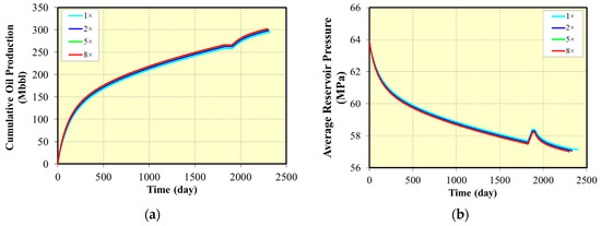
Figure 24. Effect of different permeability magnifications in the SRV region with one huff-n-puff cycle on oil production and reservoir pressure: (a) Cumulative oil production for different magnification of permeability in SRV region; (b) Average reservoir pressure for different permeability magnifications in the SRV region.

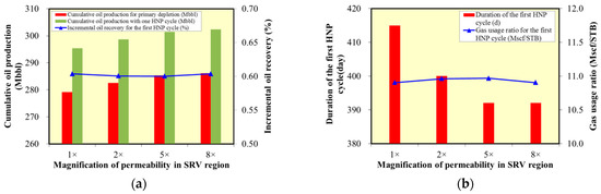
Figure 25. Correlation between magnification of permeability in SRV region and huff-n-puff results: (a) Cumulative oil production and incremental oil recovery for different magnification of permeability in SRV region; (b) Duration of the first huff-n-puff cycle and gas usage ratio for different magnification of permeability in SRV region.

As the permeability of natural fractures in the SRV region increases, the cumulative oil production during primary depletion increases, but because the area of the SRV region is small, the impact on the cumulative oil production is minor.

The increase of permeability in the SRV region has little effect on the increase in oil recovery and gas usage ratio during gas huff-n-puff.

4.3. Effect of Primary Depletion Parameters

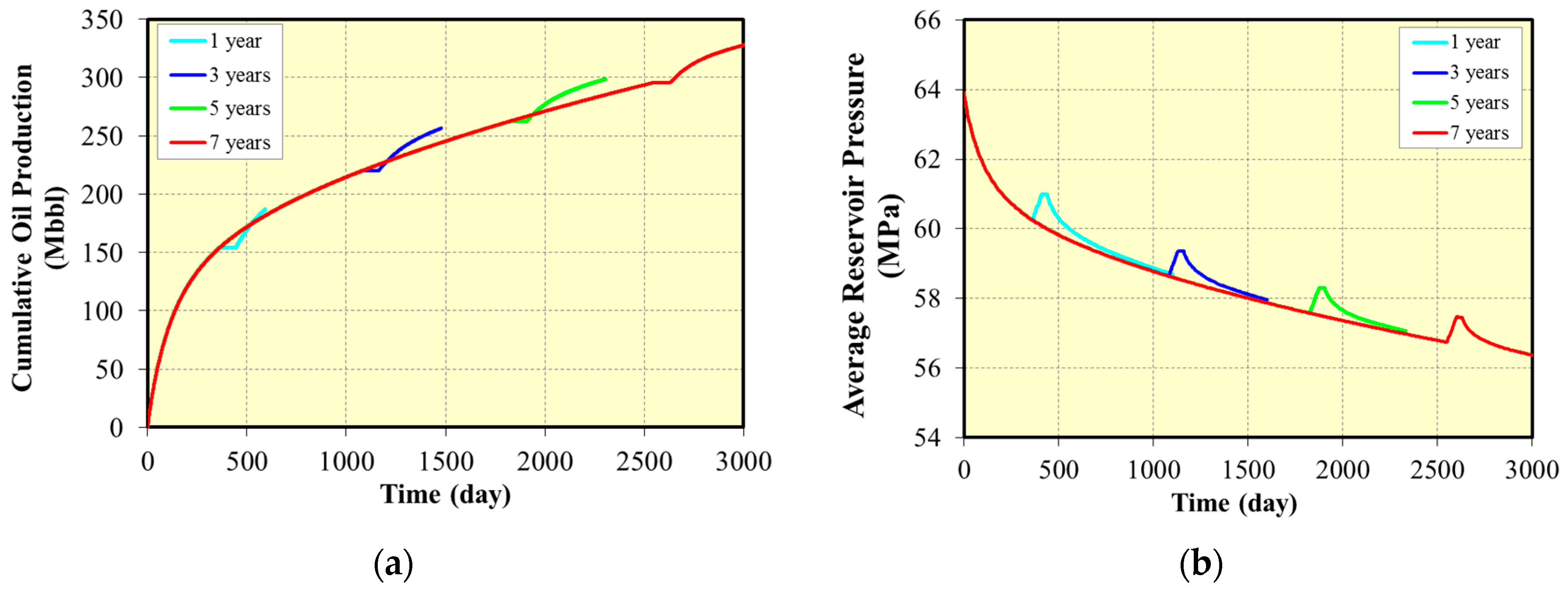
4.3.1. Period of Primary Depletion

Primary depletion has been examined for gas huff-n-puff in the period of one year, three years, five years, and seven years. The results are summarized in Table 17, and Figure 26 and Figure 27, from the figures it can be seen:

Table 17. Summary of results for huff-n-puff with different primary depletion periods.

Period of Primary Depletion (Year)	1	3	5	7
Oil rate after 5 years primary depletion (bbl/d)	154.73	66.42	50.07	42.39
Cumulative oil production for primary depletion (Mbbl)	176.99	241.33	282.55	314.41
Cumulative volume of injected gas for first huff-n-puff cycle (MMscf)	176.50	176.50	176.50	176.50
Cumulative oil production with one huff-n-puff cycle (Mbbl)	186.85	256.60	298.65	330.78
Duration of the first huff-n-puff cycle (d)	150	320	400	440
Gas usage ratio for the first huff-n-puff cycle (Mscf/STB)	17.91	11.56	10.96	10.78
Incremental oil recovery for the first huff-n-puff cycle (%)	0.37	0.57	0.60	0.61

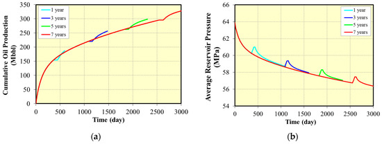
Figure 26. Effect of different periods of primary depletion with one huff-n-puff cycle on oil production and reservoir pressure: (a) Cumulative oil production for different period of primary depletion; (b) Average reservoir pressure for different period of primary depletion.

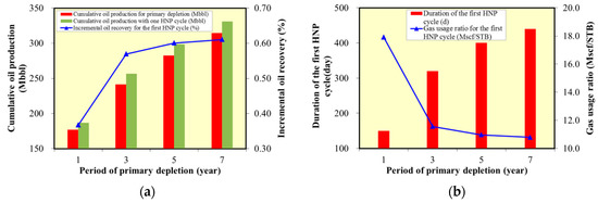
Figure 27. Correlation between the periods of primary depletion and huff-n-puff results: (a) Cumulative oil production and incremental oil recovery for different periods of primary depletion; (b) Duration of the first huff-n-puff cycle and gas usage ratio for different periods of primary depletion.

The reservoir pressure drop increases with the increase in the period of primary depletion. The incremental oil recovery also increases with the period of primary depletion.

If the gas huff-n-puff starts with a short period of primary depletion, it could result in a poor huff-n-puff effect. This is because the high reservoir pressure is not conducive to gas injection and migration to the deep part of the reservoir. At the same time, it will lead to a too high gas-oil ratio during the production stage.

The proposed period of primary depletion is five years, and the reservoir pressure should be above saturation pressure to prevent condensation in the wellbore which could affect the oil recovery.

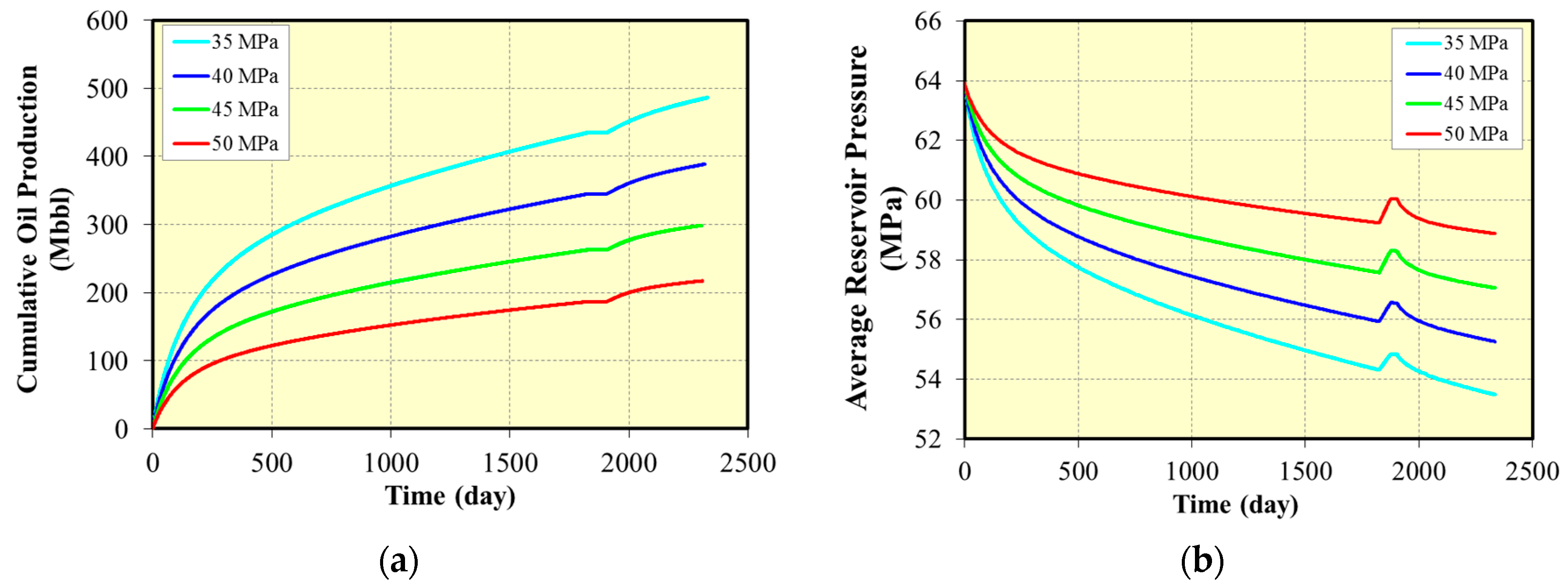
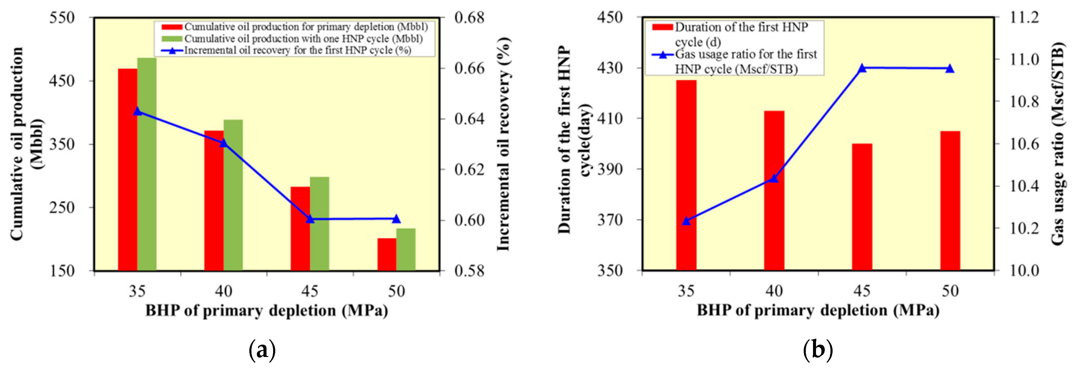
4.3.2. BHP of Primary Depletion

The bottom hole pressure (BHP) controls the well production. The lower the BHP, the greater the production pressure difference, the higher the well production, and the faster the reservoir pressure drops. In shale reservoirs, multiple studies indicated that the production characteristics of tight reservoirs with high initial production and sharp decline in production will cause irreversible damage to fractures near the wellbore and affect conductivity.

We analyzed four cases of BHP of primary depletion, which are 35 MPa, 40 MPa, 45 MPa, and 50 MPa. The base case is 45 MPa. The effect of gas huff-n-puff under different BHP of primary depletion is examined. The results are summarized in Table 18, and Figure 28 and Figure 29, it can be seen from the figures:

Table 18. Summary of results for huff-n-puff with different bottom hole pressure (BHP) of primary depletion.

BHP of Primary Depletion (MPa)	35	40	45	50
Oil rate after 5 years primary depletion (bbl/d)	81.08	65.10	50.07	35.98
Cumulative oil production for primary depletion (Mbbl)	469.09	371.61	282.55	201.11
Cumulative volume of injected gas for first huff-n-puff cycle (MMscf)	176.50	176.50	176.50	176.50
Cumulative oil production with one huff-n-puff cycle (Mbbl)	486.34	388.52	298.65	217.22
Duration of the first huff-n-puff cycle (d)	425	413	400	405
Gas usage ratio for the first huff-n-puff cycle (Mscf/STB)	10.23	10.44	10.96	10.96
Incremental oil recovery for the first huff-n-puff cycle (%)	0.64	0.63	0.60	0.60

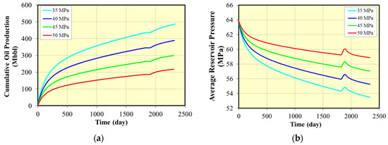
Figure 28. Effect of different BHP of primary depletion with one huff-n-puff cycle on oil production and reservoir pressure: (a) Cumulative oil production for different BHP of primary depletion; (b) Average reservoir pressure for different BHP of primary depletion.

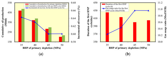
Figure 29. The correlation between BHP of primary depletion and huff-n-puff results: (a) Cumulative oil production and incremental oil recovery for different BHP of primary depletion; (b) Duration of the first huff-n-puff cycle and gas usage ratio for different BHP of primary depletion.

The incremental oil recovery increases with the decrease of BHP. This is because during primary depletion and the production period of gas huff-n-puff, the lower the BHP, the greater the pressure difference, and the higher the cumulative oil production.

The BHP should be controlled within a reasonable range. High BHP is not conducive in improving oil recovery. If BHP is too low, it will cause gas precipitation and affect the liquid phase recovery; therefore, it is recommended that the reservoir pressure should be controlled within a suitable range above the saturation pressure.

5. Results and Discussion

5.1. Sensitivity Analysis

5.1.1. Cumulative Oil Production for Primary Depletion

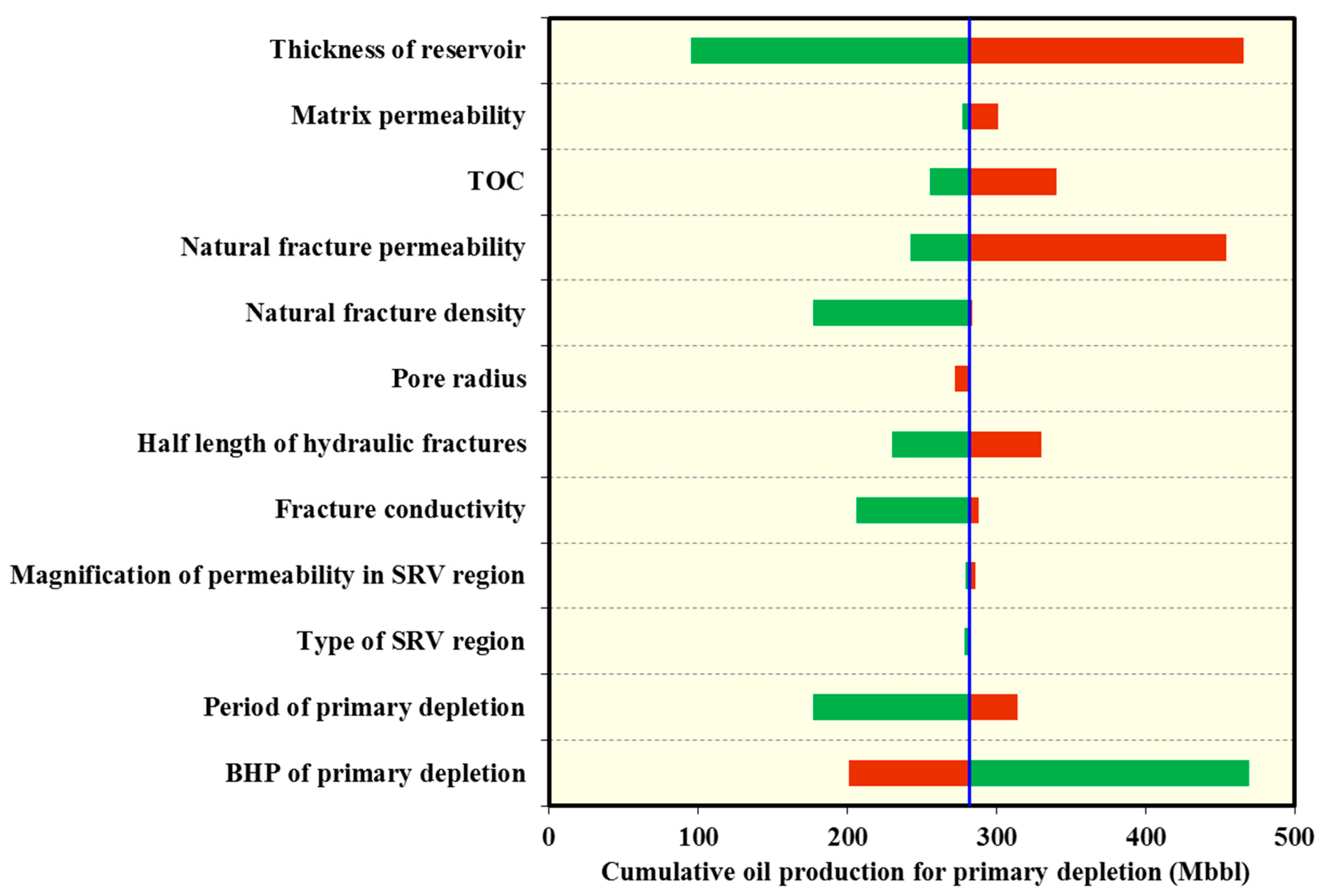
Prior to discussing the results of geological and engineering controls on gas huff-n-puff, the sensitivity of the reservoir, completion, and depletion parameters on primary production should be discussed. Figure 30 is a Tornado plot that indicates the sensitivity of the 12 parameters on cumulative oil production for primary production. The sensitivity values are measured with reference to a base model which is based on the geological features, hydraulic fracturing parameters and a good history match of primary production data. These values are obtained by setting each parameter to its minimum and maximum values one-at-a-time as shown in Table 6, while the rest of the parameters are kept at their base values. The green bars in Figure 30 correspond to the sensitivity measure (compared to the base case) when a selected parameter is set to its minimum and the red bars correspond to the sensitivity measure when a selected parameter is set to its maximum value. It can be seen from Figure 30 that reservoir thickness, BHP of primary depletion, and natural fracture permeability are recognized as the most sensitive parameters. It is followed by the period of primary depletion, half-length of hydraulic fractures, natural fracture density, TOC, fracture conductivity, and matrix permeability in order. Pore radius of shale matrix, type of SRV region, and magnification of permeability in the SRV region have the least effect on cumulative oil production for primary production. An implication of this is that these least sensitive parameters could have an insignificant impact on the gas huff-n-puff process.

Figure 30. Tornado chart indicating the most and least sensitive parameters for cumulative oil production for primary depletion. Each green bar corresponds to a sensitivity measure (compared to a base case) when a parameter is set to its lower bound. The red bars are for the upper bounds. The vertical blue line denotes the base case.

5.1.2. Incremental Oil Recovery

Multiple scenarios of compositional simulations of huff-n-puff gas injection for the proposed 12 parameters have been conducted and the incremental oil recovery for each scenario was obtained.

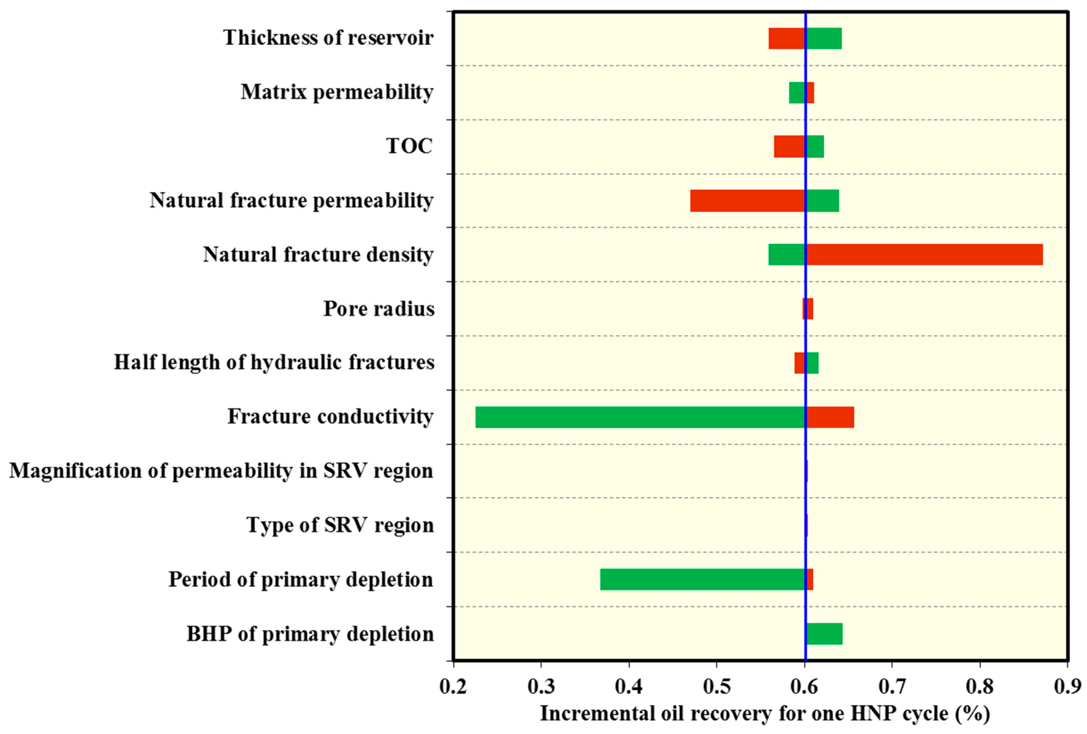
To evaluate the relative impact of the parameters, a Tornado plot (Figure 31) was created for sensitivity analysis on the incremental oil recovery. It is clear that fracture conductivity, natural fracture density, period of primary depletion and natural fracture permeability are the most sensitive parameters. It is then followed by reservoir thickness, TOC, BHP of primary depletion, matrix permeability, and half-length of hydraulic fractures in order. The effect of pore radius of shale matrix, type of SRV region and magnification of permeability in SRV region on incremental oil recovery is marginal. This rank is based on the range of each parameter listed in Table 6. The range for the percentage of recovery increase over the primary recovery for one huff-n-puff cycle (nearly 2300 days of production) is about 0.23–0.87%.

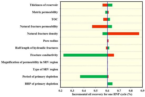
Figure 31. Tornado chart indicating the most and least sensitive parameters for incremental oil recovery. Each green bar corresponds to a sensitivity measure (compared to a base case) when a parameter is set to its lower bound. The red bars are for the upper bounds. The vertical blue line denotes the base case.

It can be seen from Figure 31 that the incremental oil recovery is positive related to natural fracture density, fracture conductivity, matrix permeability, and period of primary depletion, while it is inversely related to reservoir thickness, TOC, BHP of primary depletion, natural fracture permeability, and half-length of hydraulic fractures.

It is indicated from Figure 31 that natural fracture is key to gas huff-n-puff effectiveness. The increase of natural fracture density from 0.1 fractures/m to 0.5 fractures/m has resulted in a 0.27% increase of incremental oil recovery, which is 45% higher than the base case value (0.6%). This is attributed to a larger amount of injected gas available to contact the matrix area and extract hydrocarbons through natural fractures.

5.1.3. Gas Usage Ratio

The gas usage ratio is a key parameter to evaluate the efficiency of gas injection, which is an indicator of output-to-input ratio or economical efficiency. It is defined as the total volume of injected gas divided by total barrels of improved oil production by gas injection. For a given gas huff-n-puff scheme with a fixed composition of injected gas, a lower gas usage ratio usually implies higher economical efficiency.

Figure 32 is a Tornado plot that indicates the sensitivity of the 12 parameters on gas usage ratio for the first huff-n-puff cycle. A direct implication of Figure 32 is that low fracture conductivity and short period of primary depletion could significantly increase the gas usage ratio and result in poor economical efficiency of the gas huff-n-puff process. Nevertheless, increasing the natural fracture density could reduce the gas usage ratio. Therefore, we believe natural fractures associated with secondary hydraulic fractures (natural fractures activated by hydraulic fracturing) are the most sensitive parameters for gas huff-n-puff in Duvernay shale oil reservoirs. This is because higher fracture density (both natural fractures and hydraulic fractures) provides a much larger matrix-surface area.

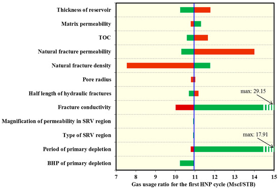
Figure 32. Tornado chart indicating the most and least sensitive parameters for gas usage ratio. Each green bar corresponds to a sensitivity measure (compared to a base case) when a parameter is set to its lower bound. The red bars are for the upper bounds. The vertical blue line denotes the base case.

5.2. Suggestions for Gas Huff-n-Puff Potential Area Screening

Based on compositional simulation of geological and engineering controls on gas huff-n-puff in Duvernay shale volatile oil reservoirs, screening criteria for gas huff-n-puff potential area are proposed. We believe that areas with higher natural fracture density, thicker reservoir, higher fracture conductivity, moderate fracture half-length, and moderate period of primary depletion are preferable for gas huff-n-puff in Duvernay shale volatile oil reservoirs to enhance oil recovery. Table 19 lists the screening criteria in the order of sensitivity for incremental oil recovery.

Table 19. Screening criteria for gas huff-n-puff potential area in Duvernay shale volatile oil reservoirs.

Sensitivity Order	Parameter	Screening Criteria
1	Fracture conductivity	≥100 mD·cm
2	Natural fracture density	≥0.1 fracture/m
3	Period of primary depletion	≥5 years
4	Natural fracture permeability	High value is preferable and more injected gas is needed for high permeability.
5	Reservoir thickness	≥30 m
6	TOC	High value is preferable.
7	Matrix permeability	≥5∙10−5 mD
8	Half-length of hydraulic fractures	Variable. Long half-length needs to inject more gas.

6. Conclusions

In this study, we built a comprehensive numerical compositional model in combination with the EDFM method that simulates the huff-n-puff gas injection process in an actual Duvernay horizontal well based on a good history match. Multiple scenarios of compositional simulations of huff-n-puff gas injection for the proposed twelve parameters have been conducted and effects of reservoir, completion, and depletion development parameters on huff-n-puff in Duvernay Shale volatile oil reservoirs are evaluated. The sensitivity of the proposed twelve parameters on cumulative oil production for primary depletion, incremental oil recovery, and gas usage ratio were examined. Moreover, we proposed a set of screening criteria for gas huff-n-puff potential areas in Duvernay shale volatile oil reservoirs. The following conclusions can be made from this study:

(1)

A complex numerical model consisting of hydraulic fractures and complex natural fractures can be easily built using the EDFM method.

(2)

Base on the actual field production data and laboratory test results, a good history match has been achieved using a comprehensive numerical compositional model in combination with the EDFM method.

(3)

The range for the recovery increase over the primary recovery for one gas huff-n-puff cycle (nearly 2300 days of production) in the Duvernay shale volatile oil reservoir is about 0.23–0.87%.

(4)

The sensitivity of the reservoir, completion, and depletion parameters on incremental oil recovery by huff-n-puff can be ranked as: fracture conductivity, natural fracture density, period of primary depletion, natural fracture permeability, reservoir thickness, TOC, BHP of primary depletion, matrix permeability and half-length of hydraulic fractures.

(5)

Sensitivity analysis indicates that natural fractures associated with secondary hydraulic fractures are the most sensitive parameters for gas huff-n-puff in Duvernay shale oil reservoirs which can be attributed to that both natural fractures and hydraulic fractures provide much larger matrix-surface area during the gas huff-n-puff process.

(6)

Screening criteria for gas huff-n-puff potential area in Duvernay shale volatile oil reservoirs are proposed. Areas with higher natural fracture density, thicker reservoir, higher fracture conductivity, moderate fracture half-length, and moderate period of primary depletion are preferable for gas huff-n-puff EOR.

(7)

A good numerical tool (EDFM) is proposed in this study that can simulate the gas Huff-n-Puff process in the shale oil reservoir with multiple hydraulic fractures and complex natural fractures more effectively and faster.

References

- LeFever, J.; Helms, L. Bakken Formation Reserve Estimates; North Dakota Geological Survey: Bismarck, ND, USA, 2008.
- Clark, A.J. Determination of Recovery Factor in the Bakken Formation, Mountrail County, ND. In Proceedings of the SPE Annual Technical Conference and Exhibition, New Orleans, LA, USA, 4–7 October 2009; Society of Petroleum Engineers (SPE): Richardson, TX, USA, 2009. [Google Scholar] [CrossRef]
- Alharthy, N.; Teklu, T.W.; Kazemi, H.; Graves, R.M.; Hawthorne, S.B.; Braunberger, J.; Kurtoglu, B. Enhanced Oil Recovery in Liquid–Rich Shale Reservoirs: Laboratory to Field. SPE Reserv. Eval. Eng. 2018, 21, 137–159. [Google Scholar] [CrossRef]
- Kathel, P.; Mohanty, K.K. EOR in Tight Oil Reservoirs through Wettability Alteration. In Proceedings of the SPE Annual Technical Conference and Exhibition, New Orleans, LA, USA, 30 September–2 October 2013; Society of Petroleum Engineers: Richardson, TX, USA, 2013. [Google Scholar] [CrossRef]
- Alvarez, J.O.; Schechter, D.S. Altering Wettability in Bakken Shale by Surfactant Additives and Potential of Improving Oil Recovery during Injection of Completion Fluids; Society of Petroleum Engineers: Richardson, TX, USA, 2016. [Google Scholar]
- Hamdi, H.; Clarkson, C.R.; Ghanizadeh, A.; Ghaderi, S.M.; Vahedian, A.; Riazi, N.; Esmail, A. Huff-N-Puff Gas Injection Performance in Shale Reservoirs: A Case Study from Duvernay Shale in Alberta, Canada. In Proceedings of the Unconventional Resources Technology Conference, Houston, TX, USA, 23–25 July 2018. [Google Scholar] [CrossRef]
- Alfarge, D.; Wei, M.; Bai, B. IOR Methods in Unconventional Reservoirs of North America: Comprehensive Review. In Proceedings of the SPE Western Regional Meeting, Bakersfield, CA, USA, 23–27 April 2017; Society of Petroleum Engineers: Richardson, TX, USA, 2017. [Google Scholar] [CrossRef]
- Davarpanah, A.; Mazarei, M.; Mirshekari, B. A simulation study to enhance the gas production rate by nitrogen replacement in the underground gas storage performance. Energy Rep. 2019, 5, 431–435. [Google Scholar] [CrossRef]
- Hu, X.; Xie, J.; Cai, W.; Wang, R.; Davarpanah, A. Thermodynamic effects of cycling carbon dioxide injectivity in shale reservoirs. J. Pet. Sci. Eng. 2020, 195, 107717. [Google Scholar] [CrossRef]
- Davarpanah, A.; Mirshekari, B. Experimental Investigation and Mathematical Modeling of Gas Diffusivity by Carbon Dioxide and Methane Kinetic Adsorption. Ind. Eng. Chem. Res. 2019, 58, 12392–12400. [Google Scholar] [CrossRef]
- Hu, X.; Li, M.; Peng, C.; Davarpanah, A. Hybrid Thermal-Chemical Enhanced Oil Recovery Methods; An Experimental Study for Tight Reservoirs. Symmetry 2020, 12, 947. [Google Scholar] [CrossRef]
- Hoffman, B. Todd. Huff-N-Puff Gas Injection Pilot Projects in the Eagle Ford. In Proceedings of the SPE Canada Unconventional Resources Conference, Calgary, AB, Canada, 13–14 March 2018. SPE-189816-MS. [Google Scholar] [CrossRef]
- Rassenfoss, S. Shale EOR Works, But Will It Make a Difference? J. Pet. Technol. 2017, 69, 34–40. [Google Scholar] [CrossRef]
- Kong, X.; Yu, W.; Wang, H.; Torres, M.; Xia, Z.; Ping, W. Compositional Simulation of Huff-n-Puff Gas Injection in a Volatile Oil Reservoir from Duvernay Shale in Alberta, Canada. In Proceedings of the 54th U.S. Rock Mechanics/Geomechanics Symposium, Golden, CO, USA, 28 June–1 July 2020. [Google Scholar]
- Ganjdanesh, R.; Yu, W.; Fiallos Torres, M.X.; Sepehrnoori, K.; Kerr, E.; Ambrose, R. Huff-N-Puff Gas Injection for Enhanced Condensate Recovery in Eagle Ford. In Proceedings of the SPE Annual Technical Conference and Exhibition, Calgary, AB, Canada, 30 September–2 October 2019; Society of Petroleum Engineers: Richardson, TX, USA, 2019. [Google Scholar] [CrossRef]
- Yu, W.; Lashgari, H.; Sepehrnoori, K. Simulation Study of CO2 Huff-n-Puff Process in Bakken Tight Oil Reservoirs. In Proceedings of the SPE Western North American and Rocky Mountain Joint Regional Meeting, Denver, CO, USA, 16–17 April 2014. SPE 169575. [Google Scholar]
- Zhang, Y.; Di, Y.; Yu, W.; Sepehrnoori, K. A Comprehensive Model for Investigation of Carbon Dioxide Enhanced Oil Recovery With Nanopore Confinement in the Bakken Tight Oil Reservoir. SPE Reserv. Eval. Eng. 2019, 22, 122–136. [Google Scholar] [CrossRef]
- Yu, W.; Zhang, Y.; Varavei, A.; Sepehrnoori, K.; Zhang, T.; Wu, K.; Miao, J. Compositional Simulation of CO2 Huff n Puff in Eagle Ford Tight Oil Reservoirs With CO2 Molecular Diffusion, Nanopore Confinement, and Complex Natural Fractures. SPE Reserv. Eval. Eng. 2019, 22, 492–508. [Google Scholar] [CrossRef]
- Song, C.; Yang, D. Performance Evaluation of CO2 Huff-n-Puff Processes in Tight Oil Formations. In Proceedings of the the SPE Unconventional Resources Conference Canada, Calgary, AB, Canada, 5–7 November 2013; Society of Petroleum Engineers: Richardson, TX, USA, 2013. [Google Scholar] [CrossRef]
- Sun, R.; Yu, W.; Xu, F.; Pu, H.; Miao, J. Compositional simulation of CO2 Huff-n-Puff process in Middle Bakken tight oil reservoir with hydraulic fracture. J. Fuel 2019, 236, 1446–1457. [Google Scholar] [CrossRef]
- Chen, C.; Balhoff, M.T.; Mohanty, K.K. Effect of Reservoir Heterogeneity on Primary Recovery and CO2 Huff-n-Puff Recovery in Shale-Oil Reservoirs. SPE Reserv. Eval. Eng. 2014, 17, 404–413. [Google Scholar] [CrossRef]
- Zhu, H.; Kong, X.; Zhao, W.; Long, H. Organic-Rich Duvernay Shale Lithofacies Classification and Distribution Analysis in the West Canadian Sedimentary Basin. In Proceedings of the International Field Exploration and Development Conference 2017; Qu, Z., Lin, J., Eds.; Springer Series in Geomechanics and Geoengineering; Springer: Singapore, 2017. [Google Scholar]
- Lyster, S.; Corlett, H.J.; Berhane, H. Hydrocarbon Resource Potential of the Duvernay Formation in Alberta–Update; Alberta Energy Regulator: Calgary, AB, Canada, 2017. [Google Scholar]
- Xu, Y.; Sepehrnoori, K. Development of an Embedded Discrete Fracture Model for Field-Scale Reservoir Simulation with Complex Corner-Point Grids. SPE J. 2019, 24, 1552–1575. [Google Scholar]
- Xu, Y.; Cavalcante Filho, J.S.A.; Yu, W.; Sepehrnoori, K. Discrete-Fracture Modeling of Complex Hydraulic-Fracture Geometries in Reservoir Simulators. SPE Reserv. Eval. Eng. 2017, 20, 403–422. [Google Scholar] [CrossRef]
- Zarragoicoechea, G.J.; Kuz, V.A. Critical Shift of a Confined Fluid in a Nanopore. Fluid Phase Equilibria 2004, 220, 7–9. [Google Scholar] [CrossRef]
- Singh, K.S.; Sinha, A.; Deo, G.; Singh, J.K. Vapor-Liquid Phase Coexistence, Critical Properties, and Surface Tension of Confined Alkanes. J. Phys. Chem. 2009, 113, 7170–7180. [Google Scholar] [CrossRef]
- Tian, H.; Zou, C.; Liu, S.; Hong, F.; Hao, J. Reservoir porosity measurement uncertainty and its influence on shale gas resource assessment. Acta Geol. Sin. 2019, 94, 233–242. [Google Scholar] [CrossRef]
- Miao, J.; Yu, W.; Xia, Z.; Zhao, W.; Xu, Y.; Sepehrnoori, K. An Easy and Fast EDFM Method for Production Simulation in Shale Reservoirs with Complex Fracture Geometries. In Proceedings of the 2nd International Discrete Fracture Network Engineering Conference, Seattle, WA, USA, 20–22 June 2018. ARMR-DFNE 18-0926. [Google Scholar]
- Yu, W.; Sepehrnoori, K. Shale Gas and Tight Oil Reservoir Simulation, 1st ed.; Elsevier: Cambridge, MA, USA, 2018; ISBN 978-0-12-813868-7. [Google Scholar]
- Kurtoglu, B.; Kazemi, H.; Rosen, R.; Mickelson, W.; Kosanke, T. A Rock and Fluid Study of Middle Bakken Formation: Key to Enhanced Oil Recovery. In Proceedings of the 76th EAGE Conference and Exhibition 2014, Amsterdam, The Netherlands, 16–19 June 2014; Society of Petroleum Engineers: Richardson, TX, USA, 2014; Volume 2014, pp. 1–5. [Google Scholar] [CrossRef]
- Luo, S.; Lutkenhaus, J.L.; Nasrabadi, H. A Framework for Incorporating Nanopores in Compositional Simulation to Model the Unusually High GOR Observed in Shale Reservoirs. In Proceedings of the SPE Reservoir Simulation Conference, Galveston, TX, USA, 10–11 April 2019. SPE-193884-MS. [Google Scholar]
- Luo, S.; Lutkenhaus, J.L.; Nasrabadi, H. Multiscale Fluid-Phase-Behavior Simulation in Shale Reservoirs Using a Pore-Size-Dependent Equation of State. SPE Reserv. Eval. Eng. 2018, 21, 806–820. [Google Scholar] [CrossRef]
- Nojabaei, B.; Johns, R.T.; Chu, L. Effect of Capillary Pressure on Phase Behavior in Tight Rocks and Shales. SPE J. 2013, 16, 281–289. [Google Scholar] [CrossRef]
Publisher’s Note: MDPI stays neutral with regard to jurisdictional claims in published maps and institutional affiliations. |
© 2021 by the authors. Licensee MDPI, Basel, Switzerland. This article is an open access article distributed under the terms and conditions of the Creative Commons Attribution (CC BY) license (https://creativecommons.org/licenses/by/4.0/).