Thermal Analysis of a Solar External Receiver Tube with a Novel Component of Guide Vanes

Abstract

The heat transfer performance of a solar external receiver tube with guide vanes was numerically studied under non-uniform heat flux conditions. Models of the smooth tube and the tube with guide vanes were built. The distributions of the temperature, velocity, turbulence intensity, and Nu predicted by these two models were compared to investigate the heat transfer enhancement and the mixing effect of the guide vanes. The effect of the Re and the α on the heat transfer enhancement was also studied. The results show that the guide vanes form spiraling flows, reduce the maximum tube and molten salt temperatures, and improve the heat transfer. In addition, a more uniform temperature distribution is achieved compared to the smooth tube, allowing the molten salt to work safely under higher heat flux conditions in the receiver tube with guide vanes. It was observed that a larger Re enhances the heat transfer on the tube wall and achieves a longer effective distance of enhanced heat transfer in the downstream region, while the spiraling flow, the heat transfer enhancement, and the mixing are stronger for a larger α.

1. Introduction

The concentrated solar power (CSP) system is a promising technology for producing electricity from solar energy and plays a significant role in the energy transformation. Among different CSP types, the solar power tower (SPT) system has received considerable attention, due to its large scale and electricity outputs, which are similar to those of conventional electricity power plants [1,2]. The SPT system mainly consists of the solar heliostats field, the receiver, the thermal storage, and the heat-to-electricity conversion system. A schematic view of an SPT power plant and pictures of the demonstration facility Solar Two can be found in Figure 1 [3].

The receiver is the key component in the solar energy-to-thermal conversion process. In several SPT projects, the external receiver has been adopted, as in the case of Solar Two [3] and SUPCON Delingha 50 MW [4]. The solar flux distributions on the receiver are usually non-uniform [5,6] because it is very difficult to concentrate the sunlight and achieve an even distribution on the surface of the receiver. The results of Besarati et al. [7] and Yao et al. [8] showed that the flux distribution was extremely non-uniform and can be approximated by a Gaussian distribution. The non-uniform solar heat flux leads to a thermal gradient in the receiver, which represents a serious problem especially in the external receiver of SPT systems, where a large heat flux on the tubes and high out-temperature of the heat transfer fluid (HTF) are generated.

The highly non-uniform heat flux and the thermal gradient may lead to high thermal stress with consequent fractures of the tubes [9]. Additionally, it also results in local over-temperatures of the HTF, which may eventually cause its thermal decomposition [10]. To solve these problems, several research works have been carried out to reduce the non-uniform temperature field, mainly by considering two approaches: the optimization of the solar flux distribution and the enhancement of the heat convection. For the optimization of the solar flux distribution on the tube surface, many studies have been based on different models such as the real-time optical model [11], coupled models based on Monte Carlo ray tracing and the finite element method [12], and the aiming strategy of heliostats [13]. For example, Sanchez-Gonzalez et al. [14] established an aiming model to optimize the concentrated points of the heliostats in SPT systems and achieved a peak heat flux reduction of 23% with slightly lower receiver interception. Gee et al. [15] and Wang et al. [16] added secondary reflectors near the absorber tube in parabolic trough collector systems to reflect sunlight to the back side of the receiver and achieve a more homogeneous solar flux distribution. However, in the case of SPT external receivers, it is very challenging to flatten the solar flux distribution on the entire surface of the tube. The reason is that mainly the half surface towards the light is heated in each tube, while the other half surface towards the back wall of the receiver is hardly heated. Additionally, the receiver tubes in SPT systems are close to each other and this makes the application of reflectors on the back side of the tubes very difficult.

Another solution for smoothing the non-uniform temperature distribution is to enhance the heat transfer on the inner tube wall and increase the transverse mixing, which would reduce the temperature gradient in the tube wall and that of the HTF. The enhancement in heat transfer convection inside a tube has been investigated and tested in the design of tubular heat exchangers [17,18]. For a tubular heat exchanger, the thermal boundary conditions are usually uniform, since the heat source is evenly distributed on the wall of the tube, as presented in the numerical work of Promvonge et al. [19], while for the external receiver tube, the thermal boundary conditions are highly non-uniform, as mentioned above. Research work has been carried out to study and optimize the internal heat transfer enhancement structures under non-uniform heat flux for the receiver tubes. Munoz et al. [20] studied the heat convection enhancement of internally helically finned tubes and investigated the effects of the number of fins and the helix angle. Their results showed that the temperature gradient is significantly reduced, and the collector efficiency increases by 3% compared to that of a smooth tube. Cheng et al. [21] showed a heat convection enhancement of the vortex generators on the inside wall of parabolic trough tubes. This was achieved by placing the vortex generators on the side of the tube exposed to the solar flux. Borunda et al. [22] analyzed and optimized the performance of a parabolic trough collector with a twisted tape insert. The results showed that the twisted tape insert reduces the peak temperature of the tube and also achieves good collector efficiencies.

Most of the research work described above was focused on heat convection enhancement at the tube wall. However, the maximum value and uniformity of temperature distributions of the tube wall and HTFs are also very important to ensure the receiver works safely, especially for molten salts [23,24], which are commonly used in SPT external receivers. The maximum working temperature of molten salts is 565 °C [25]. Therefore, the non-uniformity of the temperature distribution and the maximum temperature of the molten salt flow limit the sustainable heat flux of the receiver.

In this analysis, the external receiver tube was equipped with a novel component of guide vanes, which mix the molten salt having a different temperature in different regions of the tube, reduce transverse temperature stratification, and enhance the heat transfer. This was numerically studied under a non-uniform heat flux distribution. Firstly, two numerical models of the smooth tube and the tube with guide vanes were created. The temperatures, velocities, and Nusselt numbers predicted by these two models were analyzed and compared, in order to study the heat transfer enhancement and the mixing effect of the guide vanes. In addition, to obtain the performance of the tube with guide vanes under different flow conditions, the effect of the Reynolds number on the heat transfer enhancement was investigated. Finally, since the spin angle of the guide vane is an important geometric parameter determining the flow direction at the outlet of the guide vanes and the strength of the resulting spiraling flow, its effect on the heat transfer enhancement and the flow mixing was also studied.

2. Technical Approach

2.1. Numerical Models

The numerical models in this simulation were based on the typical tube of the external receiver of Solar Two [3], where the height and diameter of the whole receiver are 6.2 m and 5.1 m. A single tube in this receiver was selected for numerical modeling. Figure 2 shows the computational domain of the tube considered in this work, which is characterized by an additional guide vanes section. The computational domain consists of three parts, namely, the component with guide vanes, the target tube downstream of the vanes, and the preset tube upstream of the vanes. The length L of the preset tube (the preset tube is the tube in front of the vanes; its main function is to ensure that the fluid is fully developed in the component with guide vanes and in the target tube in the downstream region) was 200 mm to achieve a fully developed flow in front of the vanes. The length of the downstream target tube and the component with guide vanes was 6000 mm and 5 mm, respectively. Concerning the cross-section of the tube, the outside diameter D_t of the tube was 21 mm, and the thickness S_t of the tube wall was 1.2 mm. The geometry of the guide vanes is shown in Figure 2. The number of vanes was 8, the length in the axial direction L_b and the thickness of the vanes S_b were 5 mm and 0.5 mm, respectively, and the length in the radial direction was 8.3 mm. It was stretched twistedly with a certain spin angle α = 90° to generate the vanes. The 8 guide vanes were connected by a cylinder with a 2 mm diameter. The tube was made of stainless steel and was filled with molten salt (Solar Salt, 60% by weight NaNO₃ and 40% by weight KNO₃).

2.2. Governing Equations

The steady-state simulations in this paper were carried out by means of ANSYS Fluent 19.2 [26] (ANSYS Inc., Pittsburgh, PE, USA) on the high-performance computing (HPC) systems of Baden-Württemberg in Germany. The continuity, momentum, and energy governing equations are as follows [27]:

$$\frac{\partial \rho \overline{u_i}}{\partial x_i}=0$$

(1)

$$\rho {\overline{u}}_j\frac{\partial {\overline{u}}_i}{\partial x_j}=\rho {\overline{F}}_i-\frac{\partial \overline{p}}{\partial x_i}+\frac{\partial }{\partial x_j}\left[\mu \left(\frac{\partial {\overline{u}}_i}{\partial x_j}+\frac{\partial {\overline{u}}_j}{\partial x_i}\right)-\rho \overline{u_i^{\prime }{u}_j^{\prime }}\right]$$

(2)

$$\rho {\overline{u}}_j\frac{\partial \overline{T}}{\partial x_j}=\frac{\partial }{\partial x_j}\left(\frac{\lambda }{c_p}\frac{\partial \overline{T}}{\partial x_j}-\rho \overline{u_j^{\prime }{T}^{\prime }}\right)$$

(3)

where ρ, μ, λ, and c_p are the density, viscosity, thermal conductivity, and specific heat capacity of the molten salt, respectively. ${\overline{F}}_i$ is the body force, where the over-line denotes the average value. The term $-\rho \overline{u_i^{\prime }{u}_j^{\prime }}$ represents the Reynolds stress tensor and $\rho \overline{u_j^{\prime }{T}^{\prime }}$ expresses the turbulent heat flux.

According to the results of previous studies by A. Fritsch and coworkers [28], the k-ω turbulence model is a good choice for the simulation of the heat and mass transfers in the tube flow, and for this reason, it was adopted in these simulations. The transport equations for the turbulent kinetic energy (k) and its specific dissipation rate (ω) are expressed as [26]

$$\frac{\partial }{\partial x_i}\left(\rho k{u}_i\right)=\frac{\partial }{\partial x_j}\left[{\Gamma }_k\frac{\partial k}{\partial x_j}\right]+G_k-Y_k+S_k+G_b$$

(4)

$$\frac{\partial }{\partial x_i}\left(\rho \omega u_i\right)=\frac{\partial }{\partial x_j}\left[{\Gamma }_{\omega }\frac{\partial \omega }{\partial x_j}\right]+G_{\omega }-Y_{\omega }+S_{\omega }+G_{\omega b}$$

(5)

where G_k and G_ω are the generations of turbulence kinetic energy and ω. Γ_k and Γ_ω represent the effective diffusivity of k and ω, while Y_k and Y_ω represent the dissipation of k and ω due to the turbulence. S_k and S_ω are user-defined source terms, while G_b and G_ωb represent the buoyancy terms.

For the tube and the guide vanes which are the solid region of the computational domain, the energy transport equation under steady-state conditions is [26]

$$\nabla \cdot \left(\overrightarrow{\nu }\rho h\right)=\nabla \cdot \left(\lambda \nabla T\right)+S_{\mathrm{h}}$$

(6)

where h is the sensible enthalpy, and S_h is the volumetric heat source.

For the solution method, the simple coupling method between pressure and velocity was adopted. The second order for pressure, the second-order upwind for the momentum and energy, and the first-order upwind for the turbulent kinetic energy were considered in this simulation.

2.3. Boundary Conditions

The computation domain considered here includes the fluid domain and the tube (solid domain). For the fluid domain, the inlet was set as a mass flow inlet, with a constant mass flow rate of 1.4 kg/s. The total temperature and the turbulence intensity at the inlet were 563 K and 5%, respectively, and a constant pressure condition was assumed at the outlet. In order to simulate the non-uniformity of the solar flux on the tube wall, a cosine radial distribution of the heat flux was considered on the half surface of the tube wall (X ≥ 0), q(θ) = q_max·cos(θ), which is referred to as the heating surface (Figure 3). On the other half surface (X < 0), the adiabatic wall (the adiabatic wall is the wall with the boundary condition q_wall = 0 W/m², i.e., the heat flux through the wall is zero) condition was applied on the outer surface and this is indicated as the adiabatic surface. In the axial direction, the distribution of the heat flux was kept constant. The boundary conditions applied are summarized in

Table 1. Boundary conditions.

Parameter	Value
Inlet temperature	563 K
Mass flow rate at inlet	1.4 kg/s
Turbulence intensity at inlet	5%
Outlet pressure	1 atm
Peak heat flux qmax	800 kW/m2

.

As previously mentioned, the tube including the guide vanes was made of stainless steel and was filled with molten salt, whose thermal properties depend on the temperature. According to the literature [23], the thermal properties of the molten salt and stainless steel are those given in

Table 2. Thermal properties of the molten salt and stainless steel.

Parameter		Value
Molten salt	Density (kg/m3)	2090 − 0.636·(T − 273.15)
	Heat capacity (J/(kg·K))	1443 + 0.172·(T − 273.15)
	Heat conductivity (W/(m·K))	0.443 + 1.9 × 10−4·(T − 273.15)
	Viscosity (kg/(m·s))	0.022714 − 1.2 × 10−4·(T − 273.15) + 2.281 × 10−7·(T − 273.15) 2 − 1.474 × 10−10·(T − 273.15) 3
Stainless steel	Density (kg/m3)	8000
	Heat capacity (J/(kg·K))	500
	Heat conductivity (W/(m·K))	21.5

, where the temperature T is expressed in kelvin.

2.4. Parameter Definitions

In order to demonstrate the results clearly, a specific outside surface of the target tube S1 (0 m < Z < 1 m) and a cross-section S2 (Z = 0.25 m) were defined. In addition, the following specific lines were introduced: Line 1 (yellow color) on the outside tube surface where the heat flux reaches the peak value (X = 0.021 m, Y = 0 m, 0 m < Z < 6 m), and Line 2 (blue color) on the inner wall, with the closest position to peak heat flux (X = 0.0186 m, Y = 0 m, 0 m < Z < 6 m). The geometry of surfaces S1 and S2 and Lines 1 and 2 is shown in Figure 4.

According to previous studies [21], the Reynolds number Re is used to represent the flow state, and the Nusselt number Nu is used to represent the heat convection performance on the inside wall of the tube. Re and Nu are defined in Equations (7) and (8):

$$Re=\frac{\rho \mathrm{u}D}{\mu }$$

(7)

$$Nu=\frac{\mathrm{h}D}{{\lambda }_{\mathrm{f}}}$$

(8)

where u is the velocity of the molten salt flow at the inlet, D represents the inside diameter of the tube, h is the heat transfer coefficient on the inside wall of the tube, and λ_f is the thermal conductivity of the molten salt.

The temperature difference ΔT between the maximum and minimum temperatures on the tube cross-section is given as

$$\Delta T=T_{\max }-T_{\min }$$

(9)

The pressure drop Δp between the pressure p_b at the inlet of the guide vane component and the pressure p_out at the outlet of the tube is used to represent the flow resistance.

$$\Delta p=p_b-p_{out}$$

(10)

2.5. Discretization Mesh

Mixed discretization grids were adopted in the simulation. In the target tube and the preset tube, structured hexahedral grids were used, while for the component with guide vanes, an unstructured tetrahedral grid was applied due to the more complex structure. Firstly, the grid independence study was carried out with the total number of grid points equal to 2,709,037, 3,947,837, 5,806,037, and 7,324,537. The effect of the number of grid points on the temperature distribution on the tube surface is shown in Figure 5a. The results show that when the number of grid points equals 5,806,037, the average relative variation in the temperature is smaller than 1%, if the number of grid points continues to increase, and the positions of fluctuations also stay constant. Therefore, the discretization grid with 5,806,037 elements was adopted in the simulation, which is shown in Figure 5b. The numbers of grid points for the target tube, the component with vanes, and the preset tube are 4,648,597, 968,523, and 188,917, respectively. The dimensionless wall distance y+ was always below 1, and the grid expansion ratio from the inside wall of the tube was less than 1.2.

2.6. Operating Conditions

The heat transfer enhancement achieved by the guide vanes was investigated by comparing the smooth tube and the tube with guide vanes (α = 90°). In addition, the effect of the Re on the heat transfer was also studied. For the typical boundary conditions given in Table 1, the corresponding Re according to Equation (7) is 83,335. The cases with guide vanes (α = 90°) for different values of the Re (40,000, 60,000, 833,335, 100,000, 120,000) were simulated, corresponding to mass flow rates of 0.6727 kg/s, 1.009 kg/s, 1.4 kg/s, 1.6817 kg/s, and 2.0181 kg/s, respectively. Additionally, the effect of the spin angle α was studied. The simulated tubes are shown in Figure 6, where α is 30°, 45°, 60°, 90°, and 120°. The other geometric parameters were kept constant.

2.7. Validation of the Computational Method

To validate the accuracy of the simulation, the turbulent flow in a smooth tube based on the model developed by Fritsch et al. [28] was considered, under uniform heat flux boundary conditions on the front side of the tube. The temperature distribution at the front side of the tube obtained in this simulation and that determined by Fritsch and coworkers [28] are shown in Figure 7. The results reveal a good agreement between these two studies. The largest relative error ε₁ is 2.3% and is located at Z = 0.06 m, where the relative error ε₁ is defined as

$${\epsilon }_1=\left(T_{\mathrm{present}}-T_{Fritsch}\right)/T_{Fritsch}$$

(11)

Here, T_present and T_Fritsch are the temperatures obtained in the present work and in the work of Fritsch et al. [28], respectively.

Additionally, a comparison with the experimental results of Yang et al. [29] was also carried out. A numerical model based on the experimental model of Yang was built, and the average Nu on the inner wall of the tube was obtained for different Re numbers. The variation of the Nu with Re obtained numerically and experimentally is given in Figure 7b. The results show that the maximum and average relative errors ε₂ are 8.5% and 4.3%, which also indicates that the present simulation has a good accuracy. The relative error ε₂ is defined as

$${\epsilon }_2=\left(N{u}_{\mathrm{present}}-N{u}_{Yang}\right)/N{u}_{Yang}$$

(12)

Here, Nu_present and Nu_Yang are the average Nu on the inner wall of tube obtained in the present simulation and in the experiment of Yang et al. [29], respectively.

3. Results and Discussions

3.1. Comparison between the Tube with Guide Vanes and the Smooth Tube

Figure 8a shows the temperature contours on surface S1 and section S2 (as defined in Section 2.4) of the smooth tube (Case 1) and the tube with guide vanes (Case 2, α = 90°). The Re number in these two cases is the same, 83,335. The results show that the temperature distribution in Case 1 is highly non-uniform: the temperature is much higher on the heating surface than on the adiabatic surface (as defined in Figure 3). The temperature reaches the maximum value at the position with the peak heat flux and then decreases from this position to the opposite side along the circumferential direction. In Case 2, the temperature is much lower on the front side of the tube, where the peak heat flux occurs, and the temperature distribution across the tube cross-section is more uniform compared to that observed in Case 1. The maximum temperature T_max of the tube on S2 for Cases 1 and 2 is 694.70 K and 655.52 K, respectively, and the transverse temperature difference ΔT on S2 is 131.55 K for Case 1 and 91.14 K for Case 2. The smaller temperature difference is due to the guide vanes, which change the flow direction of the molten salt and generate a spiraling flow. This enhances the mixing within the tube and the heat convection on the tube wall, resulting in a lower maximum temperature and a more uniform temperature distribution on the tube wall. It is worth to mention that in the left side of the tube, which is close to the guide vanes in Case 2, as marked by the black square in Figure 8a, the zone of high temperature is very small and increases in size as the flow progresses downstream toward the outlet of the tube. As a consequence, the enhancement in the heat transfer decreases along the axial direction of the tube. The reason for this decrease is that the spiraling flow and mixing induced by the guide vanes become weaker due to the high viscosity of the molten salt as the flow progresses downstream.

For the fluid region of the molten salt flow, the temperature distribution in Case 1 is non-uniform and the temperature is higher in the region near the front side wall. In Case 2, the distribution is much more uniform since the guide vanes mix the downstream flow. The maximum temperatures of the molten salt flow on S2 for Cases 1 and 2 are 648.25 K and 608.88 K, respectively, and the relative variation reaches 6.47%. The average temperatures of the molten salt in Cases 1 and 2 are 567.20 K and 566.74 K. The result indicates that the guide vanes significantly reduce the maximum temperature of the molten salt flow and make the temperature distribution more uniform. Thus, the molten salt can work safely under higher heat flux conditions in the tube with guide vanes, compared to the smooth tube.

The phenomenon mentioned above can also be observed in Figure 8b,c, where the maximum temperature and the temperature difference along the tube are shown. The relative variation between the maximum temperatures in Cases 1 and 2 reaches 6.64% in the region close to the vanes and decreases to 0.55% at the position Z = 6 m (Z/D = 323). Additionally, it is worth to point out that the local tube temperature on Line 1 begins to fluctuate downstream from Z = 1.2 m in Case 2. In some positions during the region 2.5 m < Z < 3.5 m, the temperature in Case 2 is even higher than that in Case 1. Then, the fluctuation decreases rapidly from Z = 5 m, and the temperature increases smoothly again. This phenomenon can also be found in the temperature contours of the region 2 m < Z < 3 m and the region 5 m < Z < 6 m, which are given in Figure 8c. The temperature distribution has significant fluctuations and the isothermals are distributed spirally in the region 2 m < Z < 3 m, while in the region 5 m < Z < 6 m, the fluctuations disappear. This happens since the direction of the velocity is spiral, and its component along the tube is non-continuous and fluctuating. Accordingly, the heat convection performance and the wall temperature are significantly affected by the velocity, and the temperature distribution on Line 1 is fluctuating in this region.

The results further indicate that the guide vanes reduce the maximum temperature and the temperature difference on the tube. Additionally, due to the high viscosity which weakens the spiraling flow as it progresses downstream, the enhancement in the heat transfer coefficient on the tube wall decreases.

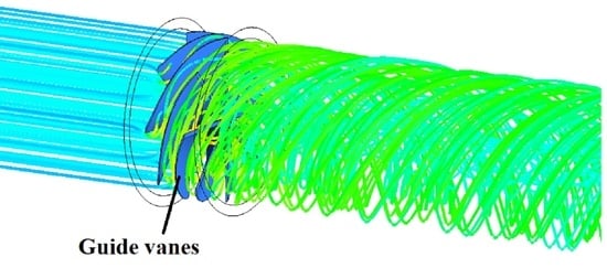
To further analyze the heat transfer enhancement of the guide vanes and the fluctuations in the temperature distribution, one should focus on the flow streamlines, the flow velocity, and the turbulence intensity presented in Figure 9 for Cases 1 and 2. The flow streamlines in Figure 9a show that the guide vane changes the direction of the velocity and forms a spiraling flow, which mixes the molten salt, reducing the temperature stratification. According to the distribution of the total velocity magnitude on section S2, which is shown in Figure 9b, for Case 2, the flow region near the wall has a higher velocity than the center of the tube, while in Case 1, the velocity in the center of the tube is higher than that in the region near the wall. The maximum velocity in Cases 1 and 2 is 3.65 m/s and 4.93 m/s, respectively, and the tangential component of the velocity on S2 in Case 2 reaches 3.73 m/s. In addition, the vectors of the total velocity presented in Figure 9c show that the velocity in Case 1 is in the axial direction, while the velocity in Case 2 is in the tangential direction. Moreover, its value and its direction change rapidly in the region near the wall. These observations indicate that the mixing influence of the guide vanes on the molten salt flow is strong.

The turbulence intensities on S2 presented in Figure 9d show that the turbulence intensity in Case 2 is much higher, especially in the region near the wall. The average turbulence intensity in Cases 1 and 2 is 15% and 26.5%, respectively. The reason is that the spiral flows enhance the disturbance, and the rapidly changed value and direction of velocity increase the turbulence intensity in the region near the wall. Since both the flow velocity and the turbulence intensity in the wall region for Case 2 are higher than those for Case 1, they lead to a significant enhancement in the heat transfer on the inside wall of the tube.

To illustrate the enhancement in the heat transfer, the distribution of the local Nu on Line 2 is given in Figure 10a. The results show that in the region 0 m < Z < 1 m, the Nu for Case 2 is on average 12.54% higher than that for Case 1. From Z = 1.2 m, the local Nu number on Line 2 for Case 2 begins to oscillate, and it decreases smoothly again from Z = 5 m, which confirms the phenomenon discussed previously. The variations in the peripherally averaged Nu (the peripherally averaged Nu is the average value of the Nu on the circle line with constant Z) numbers along the tube length for Cases 1 and 2 are shown in Figure 10b. The results show that the peripherally averaged Nu along the whole tube is higher in Case 2, especially in the region 0 m < Z < 1 m, and the average difference between Cases 1 and 2 is 9.03% in this region. The results presented above indicate that the heat convection enhancement of the guide vanes is significant in the region 0 m < Z < 1 m, and a second guide vane, placed at Z = 1 m, would be beneficial.

Besides the heat transfer enhancement, the pressure loss is also a relevant parameter for the internal structure of the tube. The average cross-sectional statistic pressures along the tubes are given in Figure 10c. It can be observed that the pressure decreases slightly in the smooth tube. In the tube with guide vanes, the pressure also decreases moderately in the preset and target tubes, but a considerable pressure drop is observed in the region with guide vanes. The pressure losses Δp₁ and Δp₂ in Cases 1 and 2 are 46.37 kPa and 108.16 kPa, respectively, and the ratio Δp₂/Δp₁ equals 2.33. The pressure loss is higher for Case 2, due to the local pressure drop of the guide vanes and the increased friction on the tube wall. This is caused by the spinning flow and the viscous friction generated by the spiraling flow.

3.2. Effect of the Re Number

Figure 11a shows the temperature contours on S1 and S2 for the Re of (40,000, 60,000, 83,335, 100,000, 120,000) and a spin angle α of 90 degrees. It can be observed that the temperature is low and distributed uniformly in the region near the vanes, while it increases and becomes non-uniform downstream. For example, for the Re equal to 40,000, a spiral characteristic of the temperature distribution is observed. As the Re increases, the maximum temperature decreases, and the temperature distribution becomes more uniform. The temperature distribution on S2 also becomes more uniform when the Re increases. The maximum tube temperature on S2 is 691.68 K, 669.43 K, 655.52 K, 649.2 K, and 643.90 K, while the temperature differences on S2 are 114.87 K, 96.97 K, 85.81 K, 80.53 K, and 76.2 K, respectively. Both temperatures decrease significantly as the Re number is increased. For the fluid region, the maximum temperature of the molten salt on S2 is 645.47 K, 623.06 K, 608.88 K, 602.52 K, and 597.14 K, respectively, i.e., it decreases as the Re number increases from 40,000 to 120,000. This happens because, for constant tube diameters, higher Re numbers correspond to higher solar salt mass flows through the tube. Since the solar flux on the tube surface is constant, the temperature decreases as the flow is increased. Higher Re numbers also increase the convection heat transfer on the tube wall.

The temperature on Line 1 and the temperature difference along the tube are presented for different Re numbers in Figure 11b,c. Both the temperature and temperature difference decrease as the Re number is increased since, as discussed previously, for constant tube diameters, higher Re numbers correspond to higher solar salt flows through the tube exposed to the constant solar flux assumed in this paper. Higher Re numbers, which correspond to higher mass flows, lead to smaller oscillations of the local temperature on Line 1 due to a stronger and more stable spiraling flow. For the highest investigated value of the Re, 120,000, the temperature oscillations are slight, and at lower Re numbers corresponding to lower solar salt flow rates, the spiraling flow is weaker and dissipates sooner due to the action of viscosity, and this causes large oscillations on the local temperatures. For Re = 40,000, the onset of local temperature oscillations is located at Z = 0.4 m, while when the Re equals 100,000, this is shifted to Z = 1.5 m.

To illustrate and analyze the effect of the Re number on the heat transfer enhancement, Figure 12a,b are provided, where the total velocity magnitude and the turbulence intensity on S2 are shown for different Re values. The results show that both the flow velocity and turbulence intensity in the region near the center of the tube, and in the region near the wall, increase significantly. The maximum flow velocity for the Re of (40,000, 60,000, 83,335, 100,000, 120,000) is 2.38 m/s, 3.6 m/s, 5.01 m/s, 6.05 m/s, and 7.27 m/s, respectively. The corresponding values of the average turbulence intensity are 12.56%, 18.26%, 24.7%, 29.08%, and 34.37%. Consequently, the increased flow velocity and turbulence intensity near the tube wall enhance the heat transfer and mix the molten salt, leading to more uniform temperatures of both the tube wall and molten salt.

The variation in the local Nu on Line 2 along the tube length for the analyzed range of Re numbers is given in Figure 13a. The results show that the Nu increases for rising Re values. As the flow progresses downstream, oscillations in the local Nu number occur due to weakening of the spiraling flow caused by viscous friction. As discussed previously, higher Re numbers result in smaller oscillations due to a stronger and more stable spiraling flow. For lower Re numbers, the spiraling flow is weaker and dissipates sooner due to the action of viscosity, resulting in large oscillations in local Nu numbers. For Re = 40,000, the onset of oscillations is located at Z = 0.4 m. This suggests that the enhancement in the heat transfer achieved by the guiding vanes is a strong function of the Re number and occurs over an effective distance, whose length also depends on the Re number. Additionally, the peripherally averaged Nu numbers along the tube length for the analyzed range of Re numbers are given in Figure 13b. The results show that the peripherally averaged Nu increases with the increase in the Re number, the average difference reaching 13.82% when the Re increases from 40,000 to 120,000.

For the analyzed tube geometry, the average Nu on the inside wall (0 m < Z < 1 m) is 31.8, 32.34, 33.41, 34.06, and 34.43 for Re values of (40,000, 60,000, 83,335, 100,000, 120,000), respectively, as shown in Figure 13c. The increase in the average Nu reaches 8.27% when the Re increases from 40,000 to 120,000. The pressure drop Δp increases with the Re number, as shown in Figure 13d. As the Re increases from 40,000 to 120,000, Δp increases from 26.66 to 216.68 kPa.

3.3. Effects of the Spin Angle

Figure 14a shows the temperature contours on the surface S1 and the cross-section S2 (Z = 0.25 m) with the spin angle α varying from 30° to 120°. The results show that, as α increases, the temperature on S1 decreases and its distribution becomes more uniform. For small values of the spin angle α, the temperature fluctuations on the tube surface along Line 1 are large, as shown in Figure 14b. As the spin angle increases, the local temperature fluctuations along Line 1 decrease in magnitude and disappear for the largest analyzed spin angle of 120 degrees. As the results show, the temperature distribution of the tube wall on S2 is also more uniform for larger α values. For an α of (30°, 45°, 60°, 90°, 120°), the maximum tube temperature shown in Figure 13b is 665.25 K, 662.29 K, 659.14 K, 655.52 K, and 644.81 K, respectively, while the corresponding temperature difference shown in Figure 13c is 94.94 K, 90.06 K, 87.56 K, 85.81 K, and 76.73 K. Both quantities decrease as the spin angle α increases. The maximum temperature of the molten salt on S2 is 619.41 K, 615.58 K, 613.37 K, 608.88 K, and 598.12 K for an α increasing from 30° to 120°. The maximum relative temperature variation reaches 4%, which means that the temperature of the molten salt flow becomes more uniform for larger α values, allowing the toleration of higher heat fluxes on the tube surface. This is because, for higher values of the α, the direction of the flow velocity is closer to the tangential flow direction, which results in a stronger spiraling flow, enhanced mixing, and a higher heat transfer enhancement.

Figure 14b also shows that for the small values of the spin angle α such as 30°, 45°, and 60°, local temperature fluctuations on Line 1 occur almost immediately downstream of the vane. As the spin angle α increases, the onset of fluctuations is pushed further downstream by the stronger spiraling flow. Thus, in terms of heat transfer enhancement, large spin angles are preferred.

To analyze this phenomenon in more detail, the distributions of the total velocity magnitude and the turbulence intensity on S2 with different spin angles α are presented in Figure 15. As the α increases and the tangential component of the flow velocity is increased, the flow velocity increases in the region near the wall and decreases in the region near the tube center. The turbulence intensity increases across the entire cross-section of the tube. For the value of the α equal to 30°, 45°, 60°, 90°, and 120°, the maximum velocity occurring near the tube wall is 4.11 m/s, 4.42 m/s, 4.76 m/s, 5.01 m/s, and 6.18 m/s, respectively, and the average turbulence intensity is 19.11%, 19.48%, 21.17%, 24.7%, and 40.36%. Both the maximum flow velocity and maximum turbulence intensity increase rapidly, especially when the α increases from 90° to 120°. For the α equal to 120°, the tangential component of the flow velocity reaches 5.15 m/s, indicating that a strong spiraling flow is formed. As discussed previously, for larger α values, the direction of the flow is close to the tangential direction, and the flow path is longer along the circumferential direction. Hence, the maximum flow velocity is higher, and the characteristics of the spiraling flow are more pronounced.

As a result of the high tangential velocity near the tube wall and the high turbulence intensity, the heat transfer on the inner wall is enhanced. The variation in the local Nu number on Line 2 along the tube length is presented in Figure 16a for different α values. Generally, the local Nu value increases with larger spin angles and reaches its highest value for the largest analyzed α (120°), which also gives a monotonic variation in the local Nu number along the tube length. The local Nu number fluctuates, with rising fluctuations for decreasing α values. Moreover, the onset of fluctuations depends on the spin angle. For small values of α, fluctuations occur almost immediately downstream from the guide vane because the spiraling flow is weak. As the α increases, and the strength of the spiraling flow increases, the onset of fluctuations occurs further downstream. Additionally, the peripherally averaged Nu numbers along the tube with the spin angle α varying from 30° to 120° are given in Figure 16b. The results show that the peripherally averaged Nu also rises with the increase in the spin angle α. In the downstream region far away from the vanes, the difference between peripherally averaged values of Nu numbers corresponding to different spin angles becomes small due to the weaker flow mixing and the smaller heat transfer enhancement in this region.

With the α varying from 30° to 120°, the average Nu on the inside wall (0 m < Z < 1 m) of the whole tube is 32.59, 32.95, 33.22, 33.41, and 34.26, respectively, as shown in Figure 16c.

The variation in pressure loss is given in Figure 16d. The results show that as the heat convection is enhanced, the pressure loss also increases. The pressure drop growth is especially large for spin angles larger than 90 degrees. Thus, when selecting the value of the α, one has to evaluate tradeoffs between the heat transfer increase and the resulting increment in the power output and pressure drop.

In general, the spin angle α has a pronounced effect on the heat transfer enhancement and on the flow mixing in the tube. For larger values of α, the tangential flow velocity is higher, and the spiraling flow is stronger, which leads to a more uniform temperature distribution of the tube wall temperature and of the molten salt flow through the tube. Additionally, the effective distance in the downstream region over which the heat transfer is increased is also longer. However, the pressure loss also increases for larger α values.

4. Conclusions

In this paper, the heat transfer performance of external receiver tubes with novel guide vane components was numerically studied. Numerical models of the smooth tube and the tube with guide vanes were built and the predicted values of the parameters of interest, such as the temperature, flow velocity, Nu, and pressure drop, were compared in order to determine the effect of the guide vanes and their geometry on the heat transfer enhancement, the flow mixing, the tube wall, and the molten salt temperature. The effect of the Reynolds number Re and the spin angle α on the heat transfer enhancement and pressure drop was also studied. The main observations can be summarized as follows:

(1) The guide vanes form a spiraling flow in the region downstream of the vane, which increases the tangential flow velocity and turbulence intensity in the region near the tube wall. This leads to the enhancement of the heat transfer and the mixing of the molten salt flow. However, the heat transfer enhancement and the flow mixing are significant in the region near the guide vanes and become weak in the downstream region. This happens because the viscous friction of the molten salt weakens the spiraling flow. As the spiraling flow becomes weaker, fluctuations in the local fluid temperature begin to occur, leading to fluctuations in the local heat transfer and in the temperature at the tube wall. Parameters such as the Reynolds number and spin angle affect the effective distance, the onset, and the strength of these fluctuations. In the tube with guide vanes, the heat transfer enhancement and the flow mixing caused by the spiral flow are significant. Therefore, the temperature distribution in this tube is more uniform, while the maximum temperature is lower compared with that in the smooth tube. This suggests that the tube with guide vanes could work under higher heat fluxes without exceeding the safe operating temperature of the tube and of the molten salt flow.

(2) The velocity, the turbulence intensity, the mass flow of the molten salt, and the heat transfer coefficient on the inner wall increase as the Re number increases. The Re number also affects the strength of the spiraling flow, increasing the heat transfer enhancement and the length of the effective distance.

(3) The spin angle α affects both the heat transfer enhancement and the pressure loss. For higher values of the α, the spiraling flow is stronger and persists over a longer length. Moreover, the tangential velocity and the turbulence intensity near the wall are stronger and lead to larger heat transfer enhancements and stronger flow mixings. However, stronger tangential velocities, especially near the wall, and the viscous friction increase the pressure drop. Thus, when selecting the value of the spin angle, one has to evaluate tradeoffs between the increase in the heat transfer and the resulting rise in the power output, as well as the growth in the pressure drop and pumping power requirements.

Future research work will focus on a two-stage spin vane system, which would be beneficial for longer tubes and tubes with a higher L/D ratio. The optimization on different spin vane angles, which can be used in the first and second stages, will be taken into account to maximize the heat transfer and minimize the pressure drop.

References

1. He, Y.-L.; Wang, K.; Qiu, Y.; Du, B.-C.; Liang, Q.; Du, S. Review of the solar flux distribution in concentrated solar power: Non-uniform features, challenges, and solutions. Appl. Therm. Eng. 2019, 149, 448–474. [Google Scholar] [CrossRef]
2. Behar, O.; Khellaf, A.; Mohammedi, K. A review of studies on central receiver solar thermal power plants. Renew. Sustain. Energy Rev. 2013, 23, 12–39. [Google Scholar] [CrossRef]
3. Pacheco, J.E. Final Test and Evaluation Results from the Solar Two Project; Sandia National Laboratories: Livermore, CA, USA, 2002; SAND-2002-0120.
4. SolarPACES. CSP Projects around the World. 2020. Available online: https://www.solarpaces.org/csp-technologies/csp-projects-around-the-world/ (accessed on 17 April 2020).
5. Farges, O.; Bézian, J.J.; Bru, H.; El Hafi, M.; Fournier, R.; Spiesser, C. Life-time integration using Monte Carlo Methods when optimizing the design of concentrated solar power plants. Solar Energy 2015, 113, 57–62. [Google Scholar] [CrossRef] [Green Version]
6. Sánchez-González, A.; Santana, D. Solar flux distribution on central receivers: A projection method from analytic function. Renew. Energy 2015, 74, 576–587. [Google Scholar] [CrossRef]
7. Besarati, S.M.; Goswami, D.Y.; Stefanakos, E.K. Optimal heliostat aiming strategy for uniform distribution of heat flux on the receiver of a solar power tower plant. Energy Convers. Manag. 2014, 84, 234–243. [Google Scholar] [CrossRef]
8. Yao, Z.; Wang, Z.; Lu, Z.; Wei, X. Modeling and simulation of the pioneer 1MW solar thermal central receiver system in China. Renew. Energy 2009, 34, 2437–2446. [Google Scholar] [CrossRef]
9. Reilly, H.E.; Kolb, G.J. An Evaluation of Molten-Salt Power Towers Including Results of the Solar Two Project; Sandia National Laboratories: Livermore, CA, USA, 2001; SAND-2001-3674.
10. Kramer, C.M.; Munir, Z.A.; Volponi, J.V. Screening test of sodium nitrite decomposition. Solar Energy Mater. 1981, 6, 85–95. [Google Scholar] [CrossRef]
11. Qiu, Y.; He, Y.-L.; Li, P.; Du, B.-C. A comprehensive model for analysis of real-time optical performance of a solar power tower with a multi-tube cavity receiver. Appl. Energy 2017, 185, 589–603. [Google Scholar] [CrossRef] [Green Version]
12. Du, B.-C.; Qiu, Y.; He, Y.-L.; Xue, X.-D. Study on heat transfer and stress characteristics of the pressurized volumetric receiver in solar power tower system. Appl. Therm. Eng. 2018, 133, 341–350. [Google Scholar] [CrossRef]
13. Garcia, J.; Barraza, R.; Too, Y.C.S. Aiming clusters of heliostats over solar receivers for distributing heat flux using one variable per group. Renew. Energy 2020, 160, 584–596. [Google Scholar] [CrossRef]
14. Sánchez-González, A.; Rodríguez-Sánchez, M.R.; Santana, D. Aiming strategy model based on allowable flux densities for molten salt central receivers. Sol. Energy 2017, 157, 1130–1144. [Google Scholar] [CrossRef]
15. Gee, R.; Winston, R. A Non-Imaging Secondary Reflector for Parabolic Trough Concentrators; Duke Solar Energy: Raleigh, NC, USA, 2001. [Google Scholar]
16. Wang, K.; He, Y.; Cheng, Z. A design method and numerical study for a new type parabolic trough solar collector with uniform solar flux distribution. Sci. China Ser. E Technol. Sci. 2014, 57, 531–540. [Google Scholar] [CrossRef]
17. Akbari, O.A.; Afrouzi, H.H.; Marzban, A.; Toghraie, D.; Malekzade, H.; Arabpour, A. Investigation of volume fraction of nanoparticles effect and aspect ratio of the twisted tape in the tube. J. Therm. Anal. Calorim. 2017, 129, 1911–1922. [Google Scholar] [CrossRef]
18. Eiamsa-Ard, S.; Thianpong, C.; Eiamsa-Ard, P.; Promvonge, P. Thermal characteristics in a heat exchanger tube fitted with dual twisted tape elements in tandem. Int. Commun. Heat Mass Transf. 2010, 37, 39–46. [Google Scholar] [CrossRef]
19. Promvonge, P.; Koolnapadol, N.; Pimsarn, M.; Thianpong, C. Thermal performance enhancement in a heat exchanger tube fitted with inclined vortex rings. Appl. Therm. Eng. 2014, 62, 285–292. [Google Scholar] [CrossRef]
20. Muñoz, J.; Abánades, A. Analysis of internal helically finned tubes for parabolic trough design by CFD tools. Appl. Energy 2011, 88, 4139–4149. [Google Scholar] [CrossRef] [Green Version]
21. Cheng, Z.; He, Y.; Cui, F. Numerical study of heat transfer enhancement by unilateral longitudinal vortex generators inside parabolic trough solar receivers. Int. J. Heat Mass Transf. 2012, 55, 5631–5641. [Google Scholar] [CrossRef]
22. Borunda, M.; Garduno-Ramirez, R.; Jaramillo, O. Optimal operation of a parabolic solar collector with twisted-tape insert by multi-objective genetic algorithms. Renew. Energy 2019, 143, 540–550. [Google Scholar] [CrossRef]
23. Benoit, H.; Spreafico, L.; Gauthier, D.; Flamant, G. Review of heat transfer fluids in tube-receivers used in concentrating solar thermal systems: Properties and heat transfer coefficients. Renew. Sustain. Energy Rev. 2016, 55, 298–315. [Google Scholar] [CrossRef]
24. Razzaghpanah, Z.; Sarunac, N. Natural convection heat transfer from a vertical column of finite number of heated circular cylinders immersed in molten solar salt. Int. J. Heat Mass Transf. 2019, 134, 694–706. [Google Scholar] [CrossRef]
25. Lata, J.M.; Rodríguez, M.; De Lara, M. Álvarez High Flux Central Receivers of Molten Salts for the New Generation of Commercial Stand-Alone Solar Power Plants. J. Sol. Energy Eng. 2008, 130, 021002. [Google Scholar] [CrossRef]
26. ANSYS Inc. ANSYS FLUENT Theory’s Guide; Release 2020 R1; ANSYS Inc.: Pittsburgh, PA, USA, 2020. [Google Scholar]
27. Chen, M.Z. Fundamentals of Viscous Fluid Dynamics; High Education Press: Beijing, China, 2002. [Google Scholar]
28. Fritsch, A.; Uhlig, R.; Marocco, L. A comparison between transient CFD and FEM simulations of solar central receiver tubs using molten salt and liquid metals. Solar Energy 2017, 155, 259–266. [Google Scholar] [CrossRef]
29. Yang, X.P.; Yang, X.X.; Ding, J. Numerical simulation study on the heat transfer characteristics of the tube receiver of the solar thermal power tower. Appl. Energy 2012, 90, 142–147. [Google Scholar] [CrossRef]
Figure 1. Schematic view and pictures of the SPT demonstration facility Solar Two [3].
Energies 14 02253 g001
Figure 2. Schematic of the receiver tube with guide vanes.
Energies 14 02253 g002
Figure 3. Distribution of the heat flux on the tube surface.
Energies 14 02253 g003
Figure 4. Schematic diagram of the specific faces and the lines on the target tube.
Energies 14 02253 g004
Figure 5. Generation and test of the numerical grid: (a) temperature on Line 1 with different grids; (b) schematic diagram of the grid.
Energies 14 02253 g005
Figure 6. Tubes with different spin angles α: (a) smooth tube; (b) α = 30°; (c) α = 45°; (d) α = 60°; (e) α = 90°; (f) α = 120°.
Energies 14 02253 g006
Figure 7. Validation of the computational method: (a) temperature distribution on the front side of the tube obtained in this simulation and in the simulation of Fritsch et al. [28]; (b) average Nu on the inner wall of tube in this simulation and in the experiment of Yang et al. [29].
Energies 14 02253 g007
Figure 8. Temperature distributions of the smooth tube and the tube with guide vanes: (a) temperature contours on S1 and S2; (b) temperature distributions on Line 1; (c) temperature differences along the tube; (d) temperature contours in downstream region of Case 2.
Energies 14 02253 g008
Figure 9. Velocity and turbulence intensity of the smooth tube and the tube with guide vanes with α = 90°: (a) flow streamlines; (b) total velocity magnitude; (c) vectors of total velocity; (d) turbulence intensity.
Energies 14 02253 g009
Figure 10. Distribution of Nu and statistic pressure in the smooth tube and the tube with guide vanes with α = 90°: (a) local Nu on Line 2; (b) peripherally averaged Nu along the tube; (c) average cross-sectional statistic pressure along the tube.
Energies 14 02253 g010
Figure 11. Temperature distributions for different Re values and α = 90°: (a) temperature contours on S1 and S2; (b) temperature distributions on Line 1; (c) temperature differences along the tube.
Energies 14 02253 g011
Figure 12. Flow velocity and turbulence intensity as a function of the Re number: (a) total velocity magnitude; (b) turbulence intensity.
Energies 14 02253 g012aEnergies 14 02253 g012b
Figure 13. Nu and Δp for different Re values and α = 90°: (a) local Nu on Line 2; (b) peripherally averaged Nu along the tube; (c) average Nu of the whole tube; (d) pressure loss.
Energies 14 02253 g013aEnergies 14 02253 g013b
Figure 14. Temperature distributions for different α values: (a) temperature contours on S1 and S2; (b) temperature distributions on Line 1; (c) temperature differences along the tube.
Energies 14 02253 g014aEnergies 14 02253 g014b
Figure 15. Flow velocity and turbulence intensity for different α values: (a) total velocity magnitude; (b) turbulence intensity.
Energies 14 02253 g015
Figure 16. Nu and Δp for different α values: (a) Nu on Line 2; (b) average Nu along the tube; (c) average Nu of whole tube; (d) pressure loss.
Energies 14 02253 g016