Perforation Optimization of Intensive-Stage Fracturing in a Horizontal Well Using a Coupled 3D-DDM Fracture Model

Abstract

Intensive-stage fracturing in horizontal wells is a potentially new technology for reservoir stimulations of deep shale oil and gas. Due to a strong stress interaction among the dense fractures, the fracture geometry and stress field are very complicated, which are the bottlenecks of this technology. Aiming at simulating the intensive-stage fracturing, a coupled three-dimensional (3D) fracture model of multiple-fracture simultaneous propagation is proposed. The dynamic behavior of the fracture propagation and stress field was analyzed using this model. The perforation parameters were optimized for improving the fracture geometry equilibrium. The results showed that the exterior fractures of the multiple fractures penetrated by the horizontal well become the main fractures, while the interior fractures are drastically restrained. The exterior fracture widths increased with increasing injection time, while the interior fracture widths decreased with increasing injection time. An extruded region was created among the multiple fractures, which restrained the propagation of the interior fractures. Only increasing the perforation cluster number did not improve the fracture geometry equilibrium in the intensive-stage fracturing. To improve the fracture geometry equilibrium, we suggest designing more perforation numbers in each perforation cluster and ensuring that both the perforation number and diameter in the interior perforation cluster are greater than those of the exterior ones.

1. Introduction

Unconventional oil and gas developments have been the most rapidly expanding trend due to a huge demand for fossil energy. The development of deep shale oil and gas has been an important area over the past few years. Hydraulic fracturing technology is widely used in enhancing shale oil and gas productions. Due to the large in-situ stress field, high clay content and low fracability in the deep area, hydraulic fracturing technology faces bottlenecks. Aiming at deep shale oil and gas reservoir simulation, field engineers try to reduce the length of each fracturing section and increase the perforation cluster number compared with those of conventional multi-stage fracturing technology. This new technology is called intensive-stage fracturing [1,2,3]. The horizontal wellbore length in each fracturing section decreases from 80–100 m to 20–25 m, while the perforation cluster spacing decreases from 30–50 m to 5–10 m [1,2]. However, the efficiency of intensive-stage fracturing technology urgently needs to be improved. Previous studies indicated that some perforation clusters could not create high-conductivity fractures or even initiate fractures [2,4,5]. This phenomenon increases the perforation cost and wastes the reservoir volume. Each fracturing section has many perforation clusters in the multi-stage fracturing technology. The stress interaction among the fractures created from the perforation cluster predominantly affects the fracture configuration [6,7,8]. Thus, building a fracture model for multi-fracture simultaneous propagation has been an urgent and hot research task over the past few years.

Extensive numerical methods were developed to model the fracture propagation, such as the extended finite element method [9,10,11], boundary element method [12,13,14], discrete element method [15,16], phase field method [17], peridynamics [18,19] and cracking particles [20], etc. Usually, in hydraulic fracture simulators, the rock is assumed to be an isotropic linear elastic medium, and thus the boundary element method constitutes an efficient method because only the boundary is discretized, and it yields accurate results for linear elastic fracture mechanics. As an indirect boundary element method, the displacement discontinuity method (DDM) has been widely used to simulate the simultaneous propagation and stress interaction of multiple 2D or pseudo-3D fractures in the same wellbore section [8,21,22,23].These studies indicated that fracture spacing is one of the most critical parameters affecting stress shadowing. Kumar [24] introduced poroelasticity to 3D fracture propagation [25,26]. These results indicated that the pore pressure could change the effective stress field and redistribute the stress field, even turning the principal stress direction by 90°. Chen et al. [27] proposed a 3D fracture model to simulate the multiple fracture propagation behavior in the multiple wells, aiming at the well factory fracturing technology. Tang [28,29] considered the fracture tortuosity and then proposed a fully 3D fracture propagation model.

In addition to the fracture model, a deeper work needs to improve the fracture geometry equilibrium after the hydraulic fracturing process. In the same fracturing section, the hydraulic fractures compete with each other such that their lengths are not even. Wu [30] employed PMMA (polymethyl methacrylate) to simulate rock samples and observed three transverse fracture propagations in the PMMA sample, and found that their fracture geometries are not even. Gunaydin et al. [4] also employed PMMA samples to simulate multiple fracture propagation and discovered a similar rule with Wu’s result [30]. The size of the exterior fracture was larger than that of the interior fracture, which suggests the existence of fracture competition behavior [30]. The exterior fracture absorbed more fluid than the interior one, so its propagation velocity was faster [4]. The interior fracture was restrained by the exterior fracture because of stress interaction. The sand slurry in the fracturing fluid with high speed eroded the perforation holes, which increased the perforation diameter and then reduced its frictional pressure loss [31]. This effect may decrease the fracture geometry equilibrium. The lower the fracture geometry equilibrium is, the more inadequate the reservoir stimulation [5]. The perforation friction can be optimized by adjusting the perforation diameter and number [5,32,33] to achieve uniform liquid injection into each perforation cluster. Li et al. [33] proposed a limited-entry multi-cluster fracturing method to improve the fracture geometry equilibrium. Cheng et al. [34,35] studied the relationship between the stage sequence and the fracture geometry in the multi-stage fracturing of a horizontal well. They indicated that both the alternative fracturing [34] and Texas two-step fracturing techniques [35] could increase the stimulated reservoir volume by improving the fracture geometry equilibrium.

Compared with conventional multi-stage fracturing technology, the perforation cluster spacing of intensive-stage fracturing technology is smaller with more perforation clusters [8,24]. The fracture geometry and stress field in intensive-stage fracturing is more complicated than before. Therefore, this paper proposes a 3D-DDM fracture model of simultaneous propagation to simulate them. To improve the fracture geometry equilibrium, this paper analyzes the fracture geometry, stress field and then optimizes the perforation parameters in a specific study site. This research may help understand reservoir stimulation in the deep shale oil and gas resources.

2. Three-Dimensional Fracture Model of Intensive-Stage Fracturing

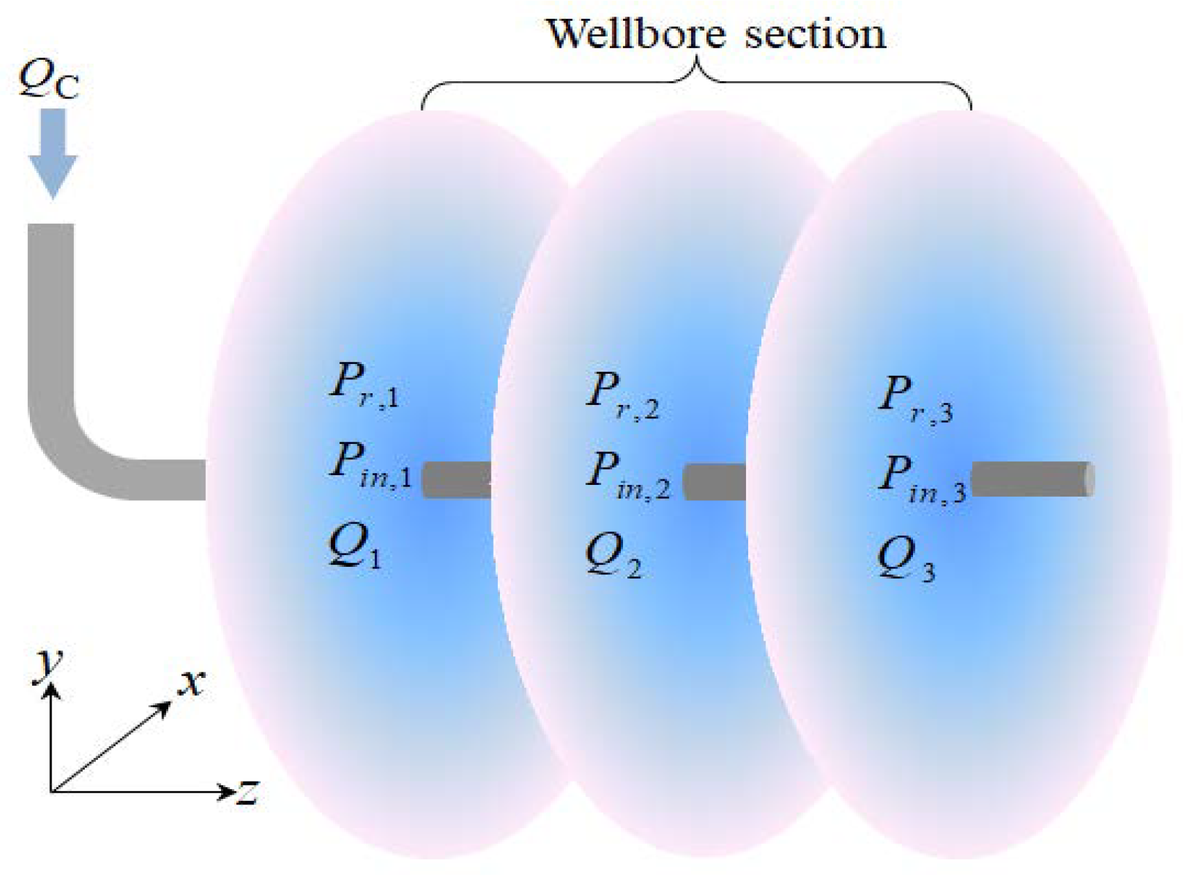
2.1. Basic Hypothesis

A sketch of intensive-stage fracturing in a horizontal well is given in Figure 1.

In intensive-stage fracturing of a horizontal well, each fracture has its own injection rate Q_k at the entry point, and the total injection rate is Q_c. The fluid partitioning is [5]:

$${\displaystyle \sum _{k=1}^{N_c}{Q}_k}=Q_c\begin{array}{cc}& \end{array}k=1,2,3,\dots ,N_c$$

(1)

where N_c is the perforation cluster number. Q_k is the injection rate into the kth fracture, m³/s. Q_c is the injection rate into the wellbore, m³/s.

Due to the flow resistance inside the fracture and the pressure drop in the perforation cluster, the fluid pressure in the wellbore is:

$$P_{w,k}=P_{r,k}+P_{in,k}\begin{array}{cc}& \end{array}k=1,2,3,\dots ,N_c$$

(2)

where P_r,_k is the pressure drop of the flow through the kth perforation cluster, Pa. P_in,_k is the flow resistance along the fracture, Pa. P_w,k is the pressure of the kth fracture at the wellbore inlet, Pa.

The perforation cluster is very closed to each other, and the frictional resistance of flowing through the casing wall is much smaller than the perforation hole friction such that the pressure is equal at every entry point [5,36]:

$$P_{w,1}=P_{w,2}=\dots =P_{w,Nc}=P_w$$

(3)

where P_w is the fluid pressure in the wellbore inlet, Pa.

To build a 3D fracture model for intensive fracture propagation, the main assumptions are as follows: ① The fracture opening and closure satisfy the linear elasticity; ② The fracture tip propagation satisfies the linear elastic fracture mechanics such that the maximum tensile stress strength criterion is selected for judging the fracture initiation and termination; ③ The fracture geometry is a planar 3D plane. Hence, a rectangular mesh can be used to discretize the fracture plane; ④ The leak-off of fracturing fluid satisfies Carter’s leak-off equation because of low permeability; ⑤ The flow resistance along the wellbore is ignored because it is much smaller than the perforation friction; ⑥ The horizontal well is assigned along the minimum horizontal principal stress, which is the general design.

2.2. Fracture Deformation

In general, the hydraulic fracture propagates along a plane perpendicular to the minimum principal stress. This plane is discretized into many rectangular meshes (Figure 2). With the injection of fracturing fluid, the meshes are activated sequentially. All the activated meshes constitute the shape of hydraulic fracture (Figure 3).

A hydraulic fracture is treated as a discontinuous displacement plane. The displacement discontinuity method (DDM) provides the displacement and stress solutions in an infinite elastic medium [12,37]. The 3D DDM is based on the elastic solution to the problem of a discontinuous displacement over a finite area in an infinite region [38]. The fundamental solutions of 3D DDM are [24,39]:

$$\{\begin{array}{l}{u}_i\left(\mathsf{\kappa }\right)={\displaystyle {\int }_{\Gamma }{U}_{ikl}\left(\mathsf{\kappa },\mathsf{\zeta }\right)D_{kl}(\mathsf{\zeta })\mathrm{d}}\Gamma \\ {\sigma }_{ij}\left(\mathsf{\kappa }\right)={\displaystyle {\int }_{\Gamma }{\Pi }_{ijkl}\left(\mathsf{\kappa },\mathsf{\zeta }\right)D_{kl}(\mathsf{\zeta })\mathrm{d}}\Gamma \end{array}\begin{array}{cc}& i,j=x,y,z\end{array}$$

(4)

where ${\Pi }_{ijkl}\left(\mathsf{\kappa },\mathsf{\zeta }\right)$ and $U_{ikl}\left(\mathsf{\kappa },\mathsf{\zeta }\right)$ are the influential coefficients of the kth displacement discontinuity of the lth fracture element on the ijth stress and the ith displacement at the location $\mathsf{\kappa }$, respectively. $D_{kl}(\mathsf{\zeta })$ is the discontinuous displacement at the location $\mathsf{\zeta }$. $\Gamma$ represents the fracture surface.

All of the hydraulic fractures have N rectangular fracture elements in total, and each element has three discontinuous displacement components D_lk (k = 1, 2, 3; l = 1, 2, 3, …, N) in the local coordinate system originated the fracture element center. The discrete form of Equation (4) is [39,40]:

$$\{\begin{array}{l}{u}_i\left(\mathsf{\kappa }\right)={\displaystyle \sum _{l=1}^N{\displaystyle \sum _{k=1}^3{U}_{ikl}\left(\mathsf{\kappa },{\mathsf{\zeta }}_l\right)}}{D}_{kl}\\ {\sigma }_{ij}\left(\mathsf{\kappa }\right)={\displaystyle \sum _{l=1}^N{\displaystyle \sum _{k=1}^3{\Pi }_{ijkl}\left(\mathsf{\kappa },{\mathsf{\zeta }}_l\right)D_{kl}}}\end{array}$$

(5)

where ${\mathsf{\zeta }}_l$ is the center of the lth fracture element.

A hydraulic fracture suffers both local and far-field stresses. The discontinuous shear displacement is assumed to be zero in this model. The physical meaning of the normal discontinuous displacement is the fracture aperture. According to Equation (5), the hydraulic fracture opening satisfies [41]:

$$p\left(\mathsf{\kappa }\right)-S_{\mathrm{h}}={\displaystyle \sum _{l=1}^N{w}_{l}C\left(\mathsf{\kappa },{\mathsf{\zeta }}_l\right)}$$

(6)

where $p\left(\mathsf{\kappa }\right)$ is the fluid pressure acting at the point $\mathsf{\kappa }$ of the fracture surface, Pa. S_h is the minimum horizontal stress, Pa. w_l is the fracture aperture of the lth fracture element, m. $C\left(\mathsf{\kappa },{\mathsf{\zeta }}_l\right)$ is the influential coefficient of the lth fracture opening on the normal stress at the fracture surface, Pa/m.

2.3. Flow of Fracturing Fluid

The friction pressure loss of a single perforation hole is [8,31]:

$$P_{r,k}=\frac{8\rho Q_k{}^2}{{\pi }^2{C}_k^2{d}_k^4{n}_k{}^2}$$

(7)

where ρ is the density of fracturing fluid, kg/m³. C_k is the dimensionless perforation coefficient. n_k is the perforation number of the kth perforation cluster. d_k is the perforation diameter of the kth perforation hole, m.

The fluid equation inside the fracture is [42]:

$$\frac{\partial w}{\partial t}+q_l=\nabla ·\left(\frac{w^3}{12u}\nabla p\right)+\delta \left(\mathsf{\kappa }-{\mathsf{\kappa }}_{in}{}_{,k}\right)\frac{Q_k}{\Delta x\Delta y}$$

(8)

where w is the fracture width, m. q_l is the leak-off velocity of the fracturing fluid, m/s. u is the viscosity of the fracturing fluid, Pa·s.

Fracturing fluid leak-off velocity is [43]:

$$q_l=\frac{2C_{lv}}{\sqrt{t-t_0}}$$

(9)

where C_lv is the leak-off coefficient, m/s^0.5. t₀ is the moment when the fracture opens, s.

Using the finite difference method, Equation (8) is divided as:

$$\begin{array}{l}\frac{w_{i,j,n+1}-w_{i,j,n}}{\Delta t}+{\displaystyle {\int }_t^{t+\Delta t}\frac{2C_{lv}}{\sqrt{t-t_0}}}\mathrm{d}t=\frac{1}{\Delta x}\left(\frac{w_{i+0.5,j,n+1}{}^3}{12u}\frac{p_{i+1,j,n+1}-p_{i,j,n+1}}{\Delta x}-\frac{w_{i-0.5,j,n+1}{}^3}{12u}\frac{p_{i,j,n+1}-p_{i-1,j,n+1}}{\Delta x}\right)\\ +\frac{1}{\Delta y}\left(\frac{w_{i,j+0.5,n+1}{}^3}{12u}\frac{p_{i,j+1,n+1}-p_{i,j,n+1}}{\Delta \mathrm{y}}-\frac{w_{i,j-0.5,n+1}{}^3}{12u}\frac{p_{i,j,n+1}-p_{i,j-1,n+1}}{\Delta y}\right)+\frac{1}{\Delta x\Delta y}{\displaystyle {\int }_t^{t+\Delta t}\delta \left(\mathsf{\kappa }-{\mathsf{\kappa }}_{in}{}_{,k}\right)Q_k}\mathrm{d}t\end{array}$$

(10)

If the square mesh (Δx = Δy) and central difference are used, Equation (10) is simplified as:

$$\begin{array}{l}\frac{w_{i,j,n+1}-w_{i,j,n}}{\Delta t}+4C_{lv}\left(\sqrt{t+\mathrm{d}t-t_0}-\sqrt{t-t_0}\right)\\ =\frac{1}{\Delta x^2}\frac{w_{i,j,n+1}{}^3}{12u}\left(p_{i+1,j,n+1}+p_{i-1,j,n+1}+p_{i,j+1,n+1}+p_{i,j-1,n+1}-4p_{i,j,n+1}\right)+\frac{\Delta t}{\Delta x^2}\delta \left(\mathsf{\kappa }-{\mathsf{\kappa }}_{in}{}_{,k}\right)Q_{k,n+1}\end{array}$$

(11)

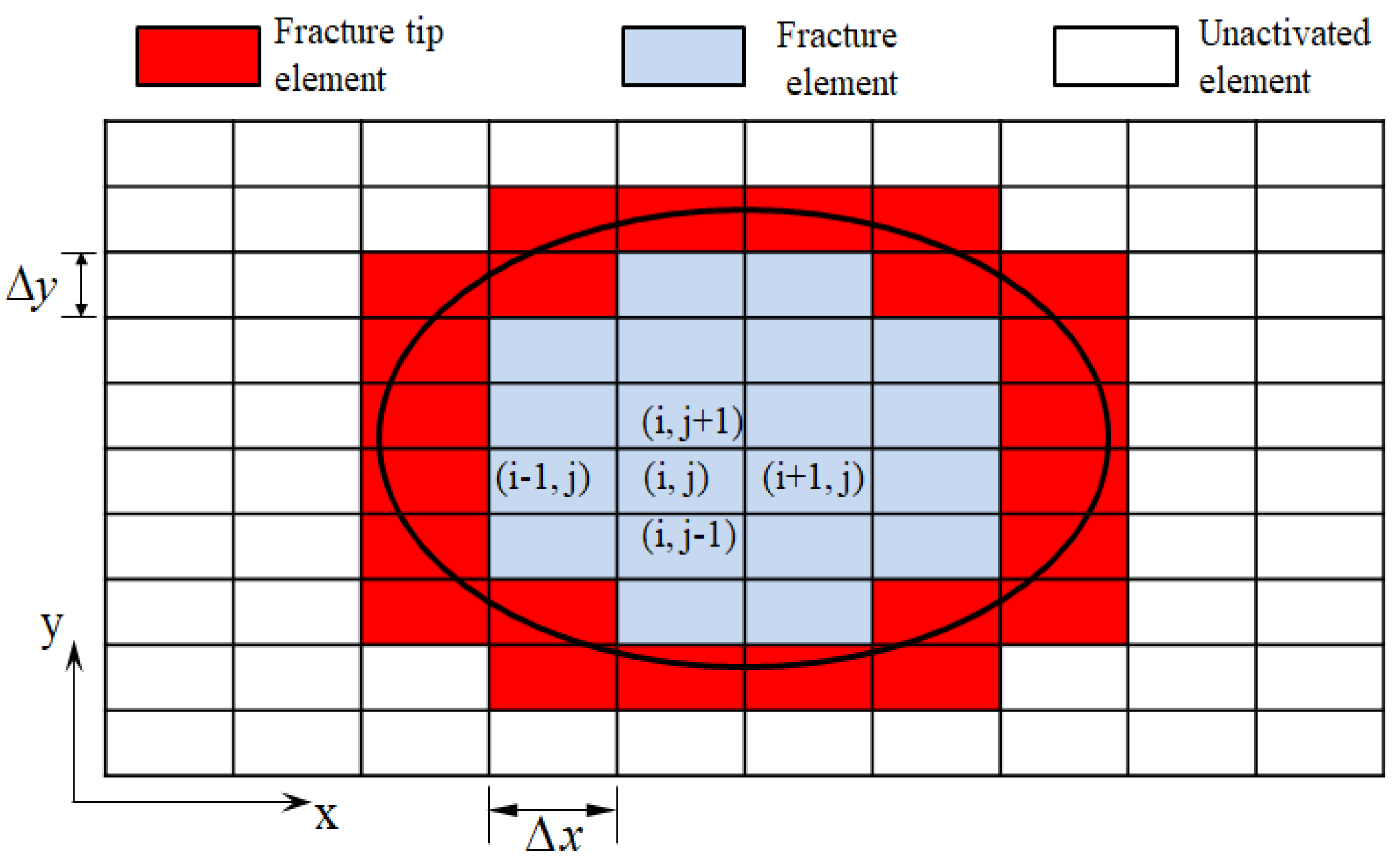
2.4. Fracture Propagation Condition

The maximum tensile stress [24] at the type-I fracture tip is:

$${\sigma }_{\theta }=\frac{K_I}{\sqrt{2\pi r}}$$

(12)

where K_I is the stress intensity factor of the type-I fracture tip, Pa·m^0.5; r, θ represent the local coordinate system originating at the fracture tip. σ_θ is the tensile stress at the fracture tip, Pa.

According to the maximum tensile strength criterion [24], the fracture will propagate when K_I > K_IC:

$${\sigma }_{\theta }>\frac{K_{IC}}{\sqrt{2\pi r}}$$

(13)

where K_IC is the fracture toughness of type-I fracture, Pa·m^0.5.

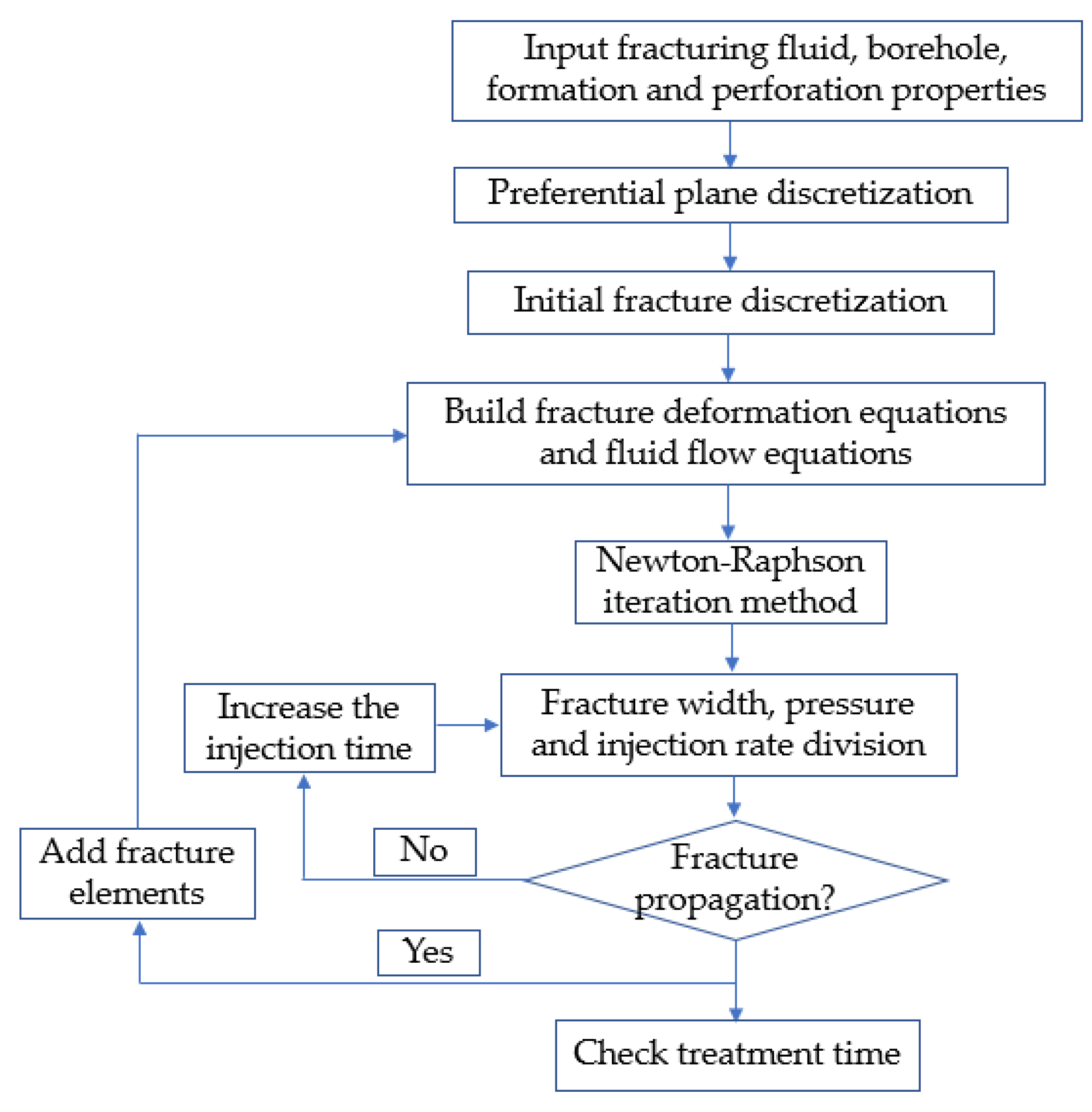
2.5. Fluid–Solid Coupling Method

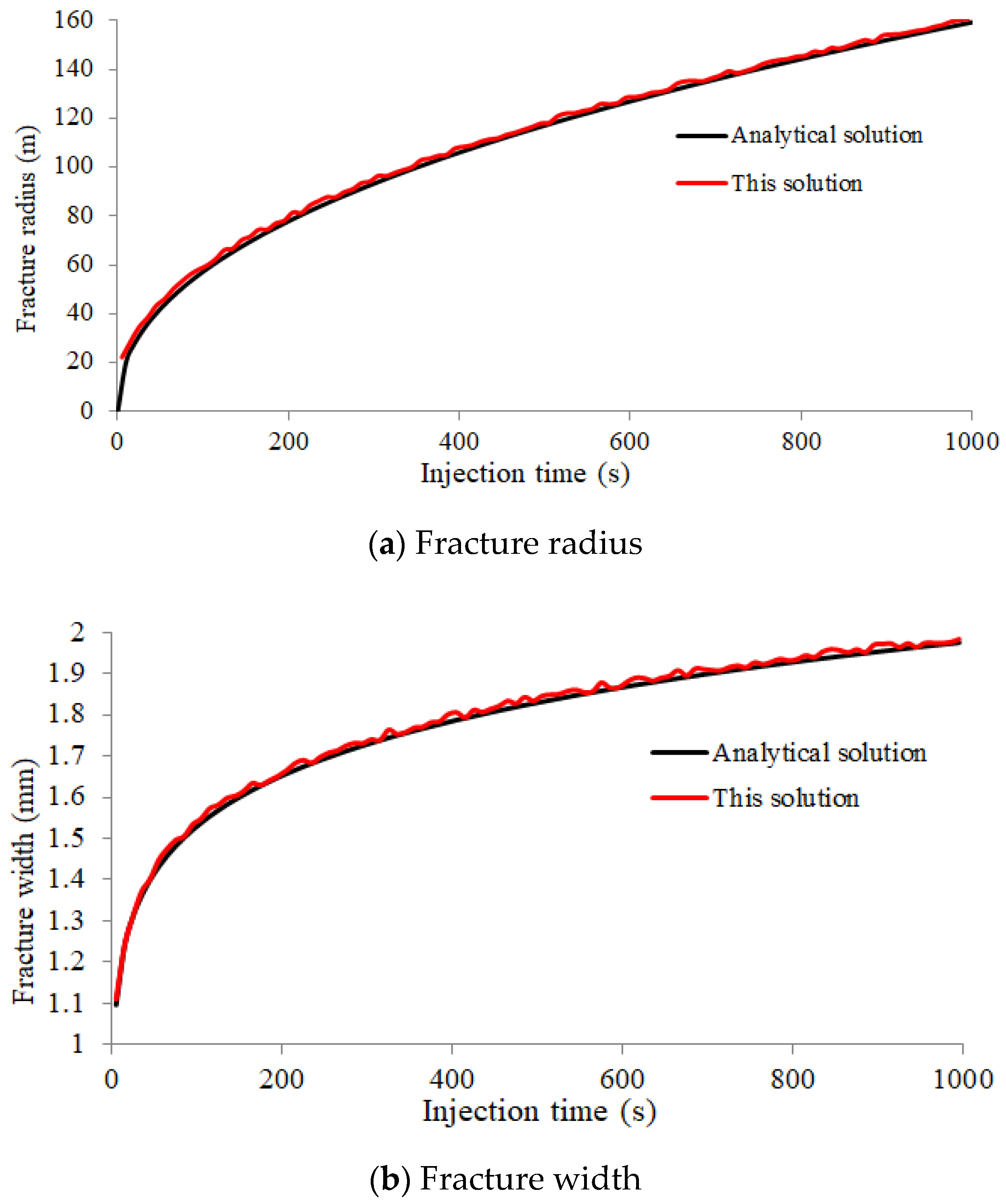
The combination of Section 2.1, Section 2.2, Section 2.3 and Section 2.4 constitutes a fluid–solid coupled 3D fracture propagation model for the simulation of intensive-stage fracturing in the horizontal well. Newton–Raphson iteration method is used to solve it. The residual function vector is:

$$F=\left[\begin{array}{cccc}{F}_1& F_2& F_3& F_4\end{array}\right]$$

(14)

where

$$\{\begin{array}{l}{F}_1=p\left(\mathsf{\kappa }\right)-S_h-{\displaystyle \sum _{l=1}^N{w}_{l}C\left(\mathsf{\kappa },{\mathsf{\zeta }}_l\right)}\\ F_2=\frac{\partial w}{\partial t}+q_l-\nabla ·\left(\frac{w^3}{12u}\nabla p\right)-\delta \left(\mathsf{\kappa }-{\mathsf{\kappa }}_{in}{}_{,k}\right)\frac{Q_k}{\Delta x\Delta y}\\ F_3={\displaystyle \sum _{k=1}^{N_c}{Q}_k}-Q_c\\ F_4=P_w-P_{r,k}-P_{in,k}\end{array}$$

(15)

The solution vector is:

$$x=\left[\begin{array}{cccc}{w}_l& p_l& Q_k& P_w\end{array}\right]\begin{array}{cc}& \end{array}l=1,2,3,\dots ,N;k=1,2,\dots ,N_c$$

(16)

The iteration format is:

$$\{\begin{array}{l}J\Delta x^{(m)}=-F(x^{(m)})\\ x^{(m+1)}=x^{(m)}+\Delta x^{(m)}\\ J=\frac{\partial F}{\partial x}\end{array}\begin{array}{ccc}& & \end{array}\left(m=0,1,2,3...\right)$$

(17)

The iteration convergence is checked by:

$${\Vert \Delta x^{(m)}\Vert }_2<0.0001\times \max \left\{x^{(m)}\right\}\begin{array}{cc}& \begin{array}{cc}or& \end{array}\end{array}{\Vert F(x^{(m)})\Vert }_2<0.0001\times \max \left\{x^{(m)}\right\}$$

(18)

The analytical solution of a penny-shaped fracture is used as x⁽⁰⁾. Once the iteration reaches convergence, the fracture element widths are used to judge the fracture tip propagation. New fracture elements are added to the fracture tip once the previous fracture tip propagates. The fracture footprint is built step-by-step (Figure 4).

2.6. Benchmarking

In the absence of fracture fluid leak-off, the analytical solutions of the fracture radius and the central fracture width of a penny-shaped fracture are [24,27]:

$$W_0(t)=2.17{\left[\frac{{(1-v^2)}^2{\mu }^2{Q}_c{}^{3}t}{E^2}\right]}^{1/9}$$

(19)

$$R(t)=0.52{\left[\frac{E{Q}_c{}^3{t}^4}{\mu (1-v^2)}\right]}^{1/9}$$

(20)

where E is Young’s modulus, Pa. t is the injection time, s. W₀ (t) is the centric width of hydraulic fracture, m. v is the Poisson’s ratio, dimensionless. R(t) is the radius of hydraulic fracture, m.

A comparison of the analytical and numerical solutions is given in Figure 5, using the input parameters in

Table 1. Input parameters for verification [27].

Parameter	Value	Parameter	Value
Elastic modulus	21 GPa	Fracturing fluid viscosity	0.6 mPa·s
Poisson’s ratio	0.2	Injection rate	5 m3/min

.

3. Fracture Geometry and Stress Field Analysis

The traditional perforation cluster spacing in the multi-stage fracturing technology is about 30–50 m, and the number of perforation clusters is about 2–3. The perforation cluster spacing declines by 5–10 m, and the number of perforation clusters increases by 5–6, which is called intensive-stage fracturing. The following cases will aim at simulating the fracture propagation and stress field in the intensive-stage fracturing technology.

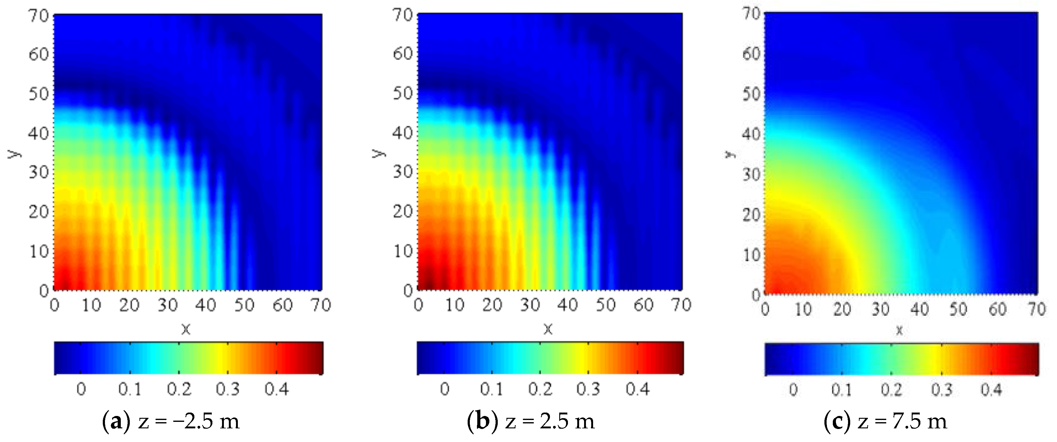
3.1. Fracture Geometry

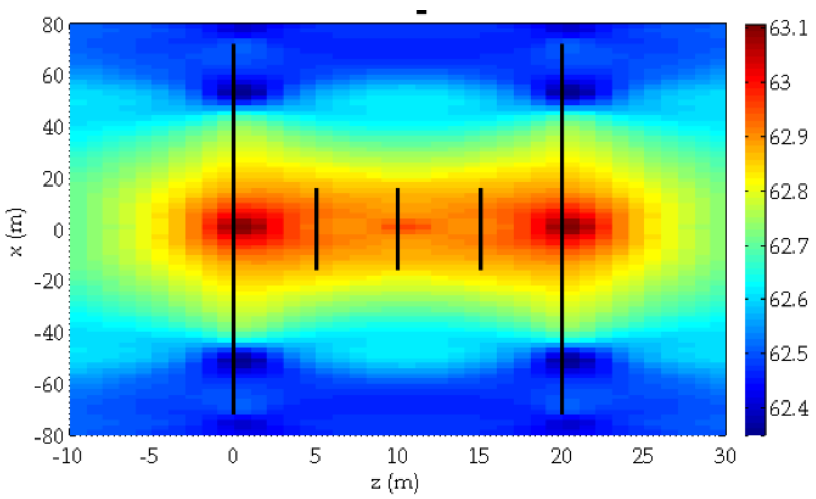
The related parameters in a deep shale oil reservoir of the Qianjiang formation, Jianghan Basin are given in

Table 2. Input parameters.

Parameter	Value	Parameter	Value
Elastic modulus	21 GPa	Fracture toughness	1 MPa·m0.5
Poisson’s ratio	0.3	Leakoff coefficient	1.5 × 10−7 m/s0.5
Fracturing fluid viscosity	20 mPa·s	Perforation cluster spacing	5 m
Injection rate	5 m3/min	Perforation cluster number	5
Minimum horizontal stress	58.5 MPa	Perforation number of each cluster	15
Maximum horizontal stress	62.5 MPa	Diameter of perforation hole	16 mm
Vertical stress	85 MPa	-	-

.

The hydraulic fracture geometry at an injection time of 5 min is given in Figure 6. The exterior fractures (fracs 1 and 5) become the main fractures with the largest widths. The interior fractures (fracs 2–4) are hardly restrained and have the smallest widths. The exterior fractures’ radii are much larger than those of the interior fractures because the interior fractures stop after a short time. The hydraulic fracture geometry is symmetrical along the x and y-axes. Wu [30] and Gunaydin et al. [4] observed multiple transverse fracture propagations in the PMMA sample, respectively. The fracture geometries in their test are very similar to our simulation results.

The time variation of the hydraulic fracturing is given in Figure 7. Due to the symmetry, the exterior fractures’ widths (fracs 1 and 5) have the same variation versus the injection time. With increasing injection time, the fracture width increases drastically in the beginning and then gradually increases. The widths of the interior fractures (fracs 2–4) decline with the injection time. In the beginning, the declining rate is much greater than that later. Due to the symmetry, fracs 2 and 4 have the same width variation. Their widths both decline to zero because of the strong stress interaction induced by the adjacent main fractures (fracs 1 and 5). Frac 3 is located in the middle area, which is far from the main fractures; hence, the stress interaction strength is weaker, and the width of frac 3 is wider than that of fracs 2 and 4.

The fluid pressure distribution inside the hydraulic fracture is given in Figure 8. The inlet pressure is the largest, while the pressure at the fracture tip is the lowest. The fluid pressure declines along the fracture radius, which indicates a penny-shaped fracture geometry. The injection pressure at the wellbore versus the injection time is given in Figure 9. The injection pressure declines rapidly in the beginning and then gradually declines later. The final pressure tends to the original minimum horizontal stress.

3.2. Stress Field

The stress distribution of S_zz is symmetrical along a plane z = 10 m (Figure 10). The S_zz in the middle area (red area in Figure 10) is much greater than the original minimum horizontal stress (S_h = 58.5 MPa). This indicates a strong compression along the z-axis in the middle area. In the area far from the horizontal well (blue area in Figure 10), S_zz is less than the original minimum horizontal stress (S_h = 58.5 MPa). This indicates a tension along the z-axis induced by the opening fracture. Due to the stress interaction, fracs 2–4 suffer strong compressive stress created by the exterior fractures, and their propagation is strongly restrained.

The stress shadowing along the z-axis induced by the opening fracture is

$$\Delta S_{\mathrm{zz}}=S_{\mathrm{zz}}-S_{\mathrm{h}}$$

(21)

Due to the symmetry of the x-axis and y-axis, the stress shadowing is also symmetrical along the x-axis and y-axis. The $\Delta S_{\mathrm{zz}}$ on 1/4 of the x–y plane is given in Figure 11. S_zz is also symmetrically distributed at a plane z = 10, so the $\Delta S_{\mathrm{zz}}$ on the planes z = −2.5 m, 2.5 m, 7.5 m are given in Figure 11a–c, respectively. $\Delta S_{\mathrm{zz}}$ on the planes z = −2.5 m, z = 2.5 m, z = 7.5 m are equal to that on the planes z = 22.5 m, z = 17.5 m, z = 12.5 m, respectively. $\Delta S_{\mathrm{zz}}$ is greater than zero in the area adjacent to the wellbore (locating on x, y = 0), while it is less than zero in the far-field area. The stress fluctuation in the area adjacent to the wellbore is caused by the stress singularity of the rectangular element in DDM. When the region is far from the hydraulic fracture surface, the stress fluctuation will disappear.

The stress distribution of S_xx is symmetrical along the plane z = 10 m, as shown in Figure 12. S_xx in the middle area (red area in Figure 12) is greater than maximum horizontal stress (S_H = 62.5 MPa). This indicates compressive behavior along the x-axis. In the area far from the wellbore (blue area), S_xx is slightly less than S_H. This indicates tensile behavior along the x-axis in the fracture tip area.

The stress shadowing along the x-axis induced by the opening fracture is

$$\Delta S_{xx}=S_{xx}-S_{\mathrm{H}}$$

(22)

$\Delta S_{xx}$ is symmetrically distributed at the x–y plane; the $\Delta S_{xx}$ on 1/4 of the x–y plane is given in Figure 11. $\Delta S_{xx}$ is also symmetrically distributed at a plane z = 10, so the $\Delta S_{xx}$ on the z = −2.5 m, 2.5 m, 7.5 m planes are given in Figure 13a–c, respectively. $\Delta S_{xx}$ is greater than zero in the area adjacent to the wellbore, while it is less than zero in the far-field area. Therefore, an open hydraulic fracture creates stress shadowing on both the maximum and minimum horizontal stress directions.

The horizontal stress contrast coefficient after hydraulic fracturing is defined as:

$$K_{\mathrm{Hh}}=\frac{S_{xx}-S_{\mathrm{zz}}}{S_{\mathrm{H}}-S_{\mathrm{h}}}$$

(23)

The horizontal stress contrast coefficient is less than 1 in the middle area (blue area in Figure 14). It indicates that the horizontal stress contrast in the middle area declines after the hydraulic fracturing process. The horizontal stress contrast coefficient decreases when the area is close to the wellbore. The horizontal stress contrast coefficient is greater than 1 in the area far from the wellbore (red area in Figure 14). This indicates that the horizontal stress contrast in the far-field increases after the hydraulic fracturing process. Previous studies have shown that the probability of creating a complex fracture network increases with decreasing horizontal stress contrast. Hence, the area close to the wellbore is more likely to include a complex fracture network after the intensive-stage fracturing process.

4. Perforation Parameter Optimization

4.1. Perforation Number Optimization

It is assumed that a horizontal well section is perforated in 3 clusters with perforation cluster spacing of 10 m. The injection volume is 50 m³. We only change the perforation number of each perforation cluster into

Table 3. Fracture geometries under different perforation numbers.

No.	Perforation Number of 3 Clusters	Centric Width of Fracture (mm)	Fracture Surface Area (m2)
1	10, 10, 10	2.3, 0.4, 2.3	8950, 1211, 8950
2	15, 15, 15	2.4, 0.3, 2.4	10,925, 1125, 10,925
3	20, 20, 20	2.45, 0.3, 2.45	11,525, 1125, 11,525
4	10, 15, 10	2.4, 0.3, 2.4	8325, 1325, 8325
5	10, 20, 10	2.42, 0.25, 2.42	8205, 1450, 8205
6	15, 10, 15	2.35, 0.23, 2.35	9488, 1104, 9488
7	15, 20, 15	2.35, 0.25, 2.35	9985, 1255, 9985
8	20, 10, 20	2.35, 0.23, 2.35	9488, 1104, 9488
9	20, 15, 20	2.35, 0.22, 2.35	9988, 1114, 9988

. The rest parameters are listed in Table 2. Fracture width and surface area are given in Table 3.

According to the perforation number distribution, the data in Table 3 are divided into 4 groups, and each group includes 3 simulation results: group 1 (no. 1, 2 and 3); group 2 (no. 1, 4 and 5); group 3 (no. 6, 2 and 7); group 4 (no. 8, 9 and 3).

Group 1: The perforation numbers in this group are equally distributed. The exterior fracture surface area and its centric width increase with the increase of perforation number. The interior fracture surface area and centric width have the tendency to decrease with the increase of perforation number.

Group 2: We retain the exterior perforation number and increase the interior perforation number. The centric width of interior fracture decreases, and the centric width of exterior fracture increases with the increase of interior perforation number. The interior fracture surface area increases, and the exterior one decreases with the increase of interior perforation number. Increasing the perforation number of the interior perforation cluster, the equilibrium of fracture geometry is better. The higher the ratio of interior perforation number to exterior perforation number, the better the fracture geometry equilibrium. A similar rule can be observed in groups 3 and 4.

To improve the fracture geometry equilibrium, it is suggested to design enough perforation numbers in each perforation cluster and make sure that the perforation number in the interior perforation cluster is greater than that of the exterior ones.

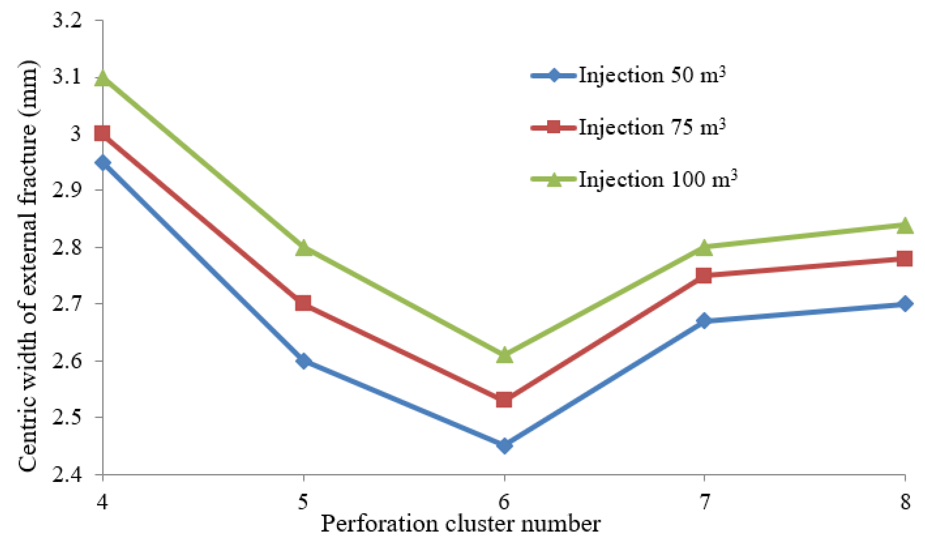
4.2. Perforation Cluster Number Optimization

It is assumed that the perforation cluster spacing is 10 m. The total injection volume of each simulation case is 50 m³. We only change the perforation cluster number, and the rest parameters are listed in Table 2. Fracture surface areas under different perforation cluster numbers and different injection volumes are listed in

Table 4. Fracture geometries under different perforation cluster numbers.

Perforation Cluster Number	Injection Volume (m3)	Centric Width of Fracture (mm)	Fracture Surface Area (m2)
4	50	2.95, 0.18, 0.18, 2.95	13,200, 1104, 1104, 13,200
	75	3.0, 0.2, 0.2, 3.0	21,328, 1104, 1104, 21,328
	100	3.1, 0.2, 0.2, 3.1	34,128, 1104, 1104, 34,128
5	50	2.6, 0.06, 0.1, 0.06, 2.6	29,968, 1104, 1104, 1104, 29,968
	75	2.7, 0.05, 0.1, 0.05, 2.7	43,472, 1104, 1104, 1104, 43,472
	100	2.8, 0.05, 0.1, 0.05, 2.8	54,416, 1104, 1104, 1104, 54,416
6	50	2.45, 0.08, 0.45, 0.45, 0.08, 2.45	27,024, 1552, 1232, 1232, 1552, 27,024
	75	2.53, 0.08, 0.43, 0.43, 0.08, 2.53	40,656, 1552, 1232, 1232, 1552, 40,656
	100	2.61, 0.08, 0.43, 0.43, 0.08, 2.61	53,625, 1552, 1232, 1232, 1552, 53,625
7	50	2.67, 0.05, 0.1, 0.1, 0.1, 0.05, 2.67	25,040, 1104, 1104, 1104, 1104, 1104, 25,040
	75	2.75, 0.05, 0.1, 0.1, 0.1, 0.05, 2.75	37,480, 1104, 1104, 1104, 1104, 1104, 37,480
	100	2.8, 0.05, 0.1, 0.1, 0.1, 0.05, 2.8	49,480, 1104, 1104, 1104, 1104, 1104, 49,480
8	50	2.7, 0.05, 0.1, 0.1, 0.1, 0.1, 0.05, 2.7	24,464, 1104, 1104, 1104, 1104, 1104, 1104, 24,464
	75	2.78, 0.04, 0.1, 0.1, 0.1, 0.1, 0.04, 2.78	35,344, 1104, 1104, 1104, 1104, 1104, 1104, 35,344
	100	2.84, 0.04, 0.1, 0.1, 0.1, 0.1, 0.04, 2.84	41,296, 1104, 1104, 1104, 1104, 1104, 1104, 41,296

. The area of the exterior fracture is still greater than that of the interior one. This phenomenon was proven by the experiments [4,30].

As shown in Table 4, the total fracture surface area in each fracturing stage is given in Figure 15. The total fracture surface area reaches the peak value when the perforation cluster number is 5. The total fracture surface area decreases linearly when the perforation cluster number is greater than 5. The total fracture surface area increases with the increase of injection volume of fracturing fluid. Only increasing the perforation cluster number cannot improve the fracture geometry equilibrium. It is suggested to optimize the perforation cluster number and perforation number in each cluster, aiming at improving the injection rate of the interior fractures. Pushing the fracturing fluid into the interior perforation hole by dropping a degradable ball to seal the exterior perforation hole may be a good choice for improving the fracture geometry equilibrium.

As shown in Table 4, the centric width of exterior fracture in each stage is given in Figure 16. The centric width of exterior fracture reaches the minimum value when the perforation cluster number is 6. The more the injection volume, the wider the centric width of the exterior fracture. A wider width contributes to the proppant migration, and the perforation cost of the 5-cluster is cheaper than that of the 6-cluster. Therefore, the best choice in this study site is to use the 5-cluster perforation for improving the stimulation efficiency.

4.3. Perforation Hole Diameter Optimization

It is assumed that a horizontal well section is perforated in 3 clusters with a spacing of 10 m. The injection volume is 100 m³. The perforation number of each cluster is 10. The rest parameters are listed in Table 2. We only use the perforation diameter in

Table 5. Fracture geometries under different perforation numbers.

No.	Perforation Diameter (mm)	Centric Width of Fracture (mm)	Fracture Surface Area (m2)
1	12, 12, 12	3.2, 0.3, 3.2	30,100, 1125, 30,100
2	14, 14, 14	2.7, 0.4, 2.7	32,696, 1552, 32,696
3	16, 16, 16	2.5, 0.8, 2.5	37,400, 1552, 37,400
4	12, 14, 12	2.9, 0.45, 2.9	37,400, 1525, 37,400
5	12, 16, 12	2.8, 0.95, 2.8	39,000, 1525, 39,000
6	14, 12, 14	3.2, 0.3, 3.2	31,700, 1025, 31,700
7	14, 16, 14	2.6, 0.85, 2.6	37,400, 1552, 37,400
8	16, 12, 16	3.2, 0.25, 3.2	32,600, 985, 32,600
9	16, 14, 16	2.9, 0.4, 2.9	35,100, 1155, 35,100

to research the relationship among the fracture width, fracture area and the perforation diameter distribution. According to the perforation diameter, the data in Table 5 are divided into 4 groups, and each group includes 3 simulation results: group 1 (no. 1, 2 and 3); group 2 (no. 1, 4 and 5); group 3 (no. 6, 2 and 7); group 4 (no. 8, 9 and 3).

Group 1: The perforation diameters in this group are equally distributed. The exterior fracture area increases with the increase of perforation diameter. The centric width of the exterior fracture decreases, and the centric width of the interior fracture increases with perforation diameter. The surface area of exterior fracture increases with the increase of perforation diameter. Under equal diameter of perforation, the fracture geometry equilibrium is better when the perforation diameter is bigger.

Group 2: We retain the exterior perforation diameter and increase the interior perforation diameter. The centric width of interior fracture decreases, and the centric width of exterior fracture increases with the increase of interior perforation number. The surface area of exterior fracture increases with the increase of interior perforation diameter. Increasing the perforation diameter of the interior perforation cluster, the equilibrium of fracture geometry is better. The higher the ratio of interior perforation diameter to exterior perforation diameter, the better the fracture geometry equilibrium. A similar rule can be observed in groups 3 and 4.

5. Conclusions

This paper proposes a coupled fracture model for the intensive-stage fracturing technology based on the 3D-DDM. It can simulate the fracture geometry and stress field in the intensive-stage fracturing of horizontal wells. Some interesting findings are:

(1)

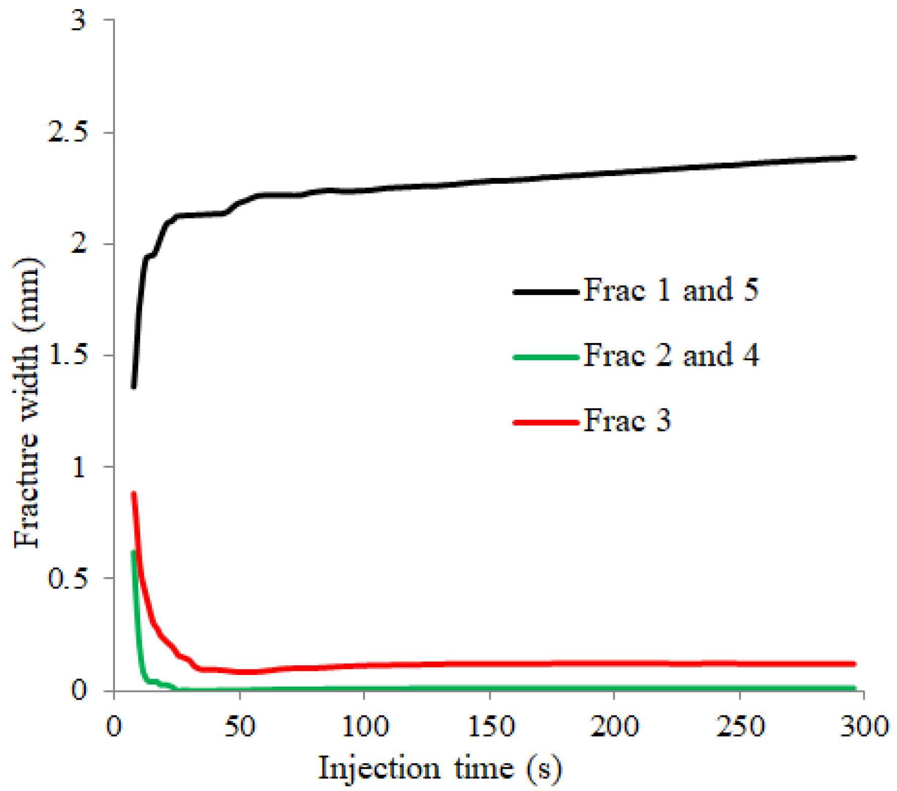
Under the uniform perforation parameters, the exterior fractures become the main fractures with the largest widths, while the interior fractures are strongly restrained and have the smallest widths. The fracture geometry equilibrium is very low under the uniform perforation parameters. Due to the symmetry, the exterior fractures’ widths have the same variation versus the injection time. With increasing injection time, the fracture width increases drastically in the beginning and then gradually increases.

(2)

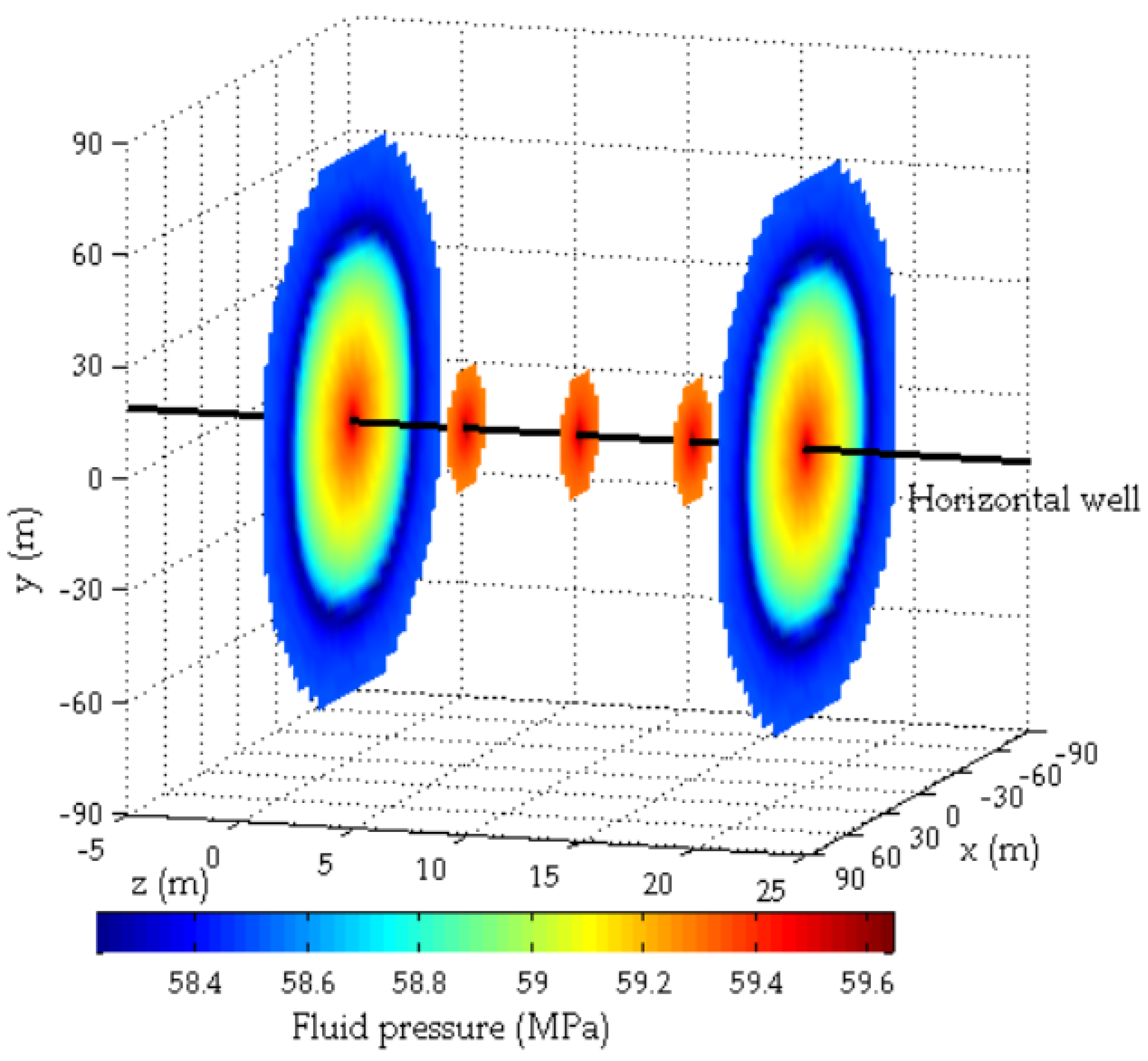
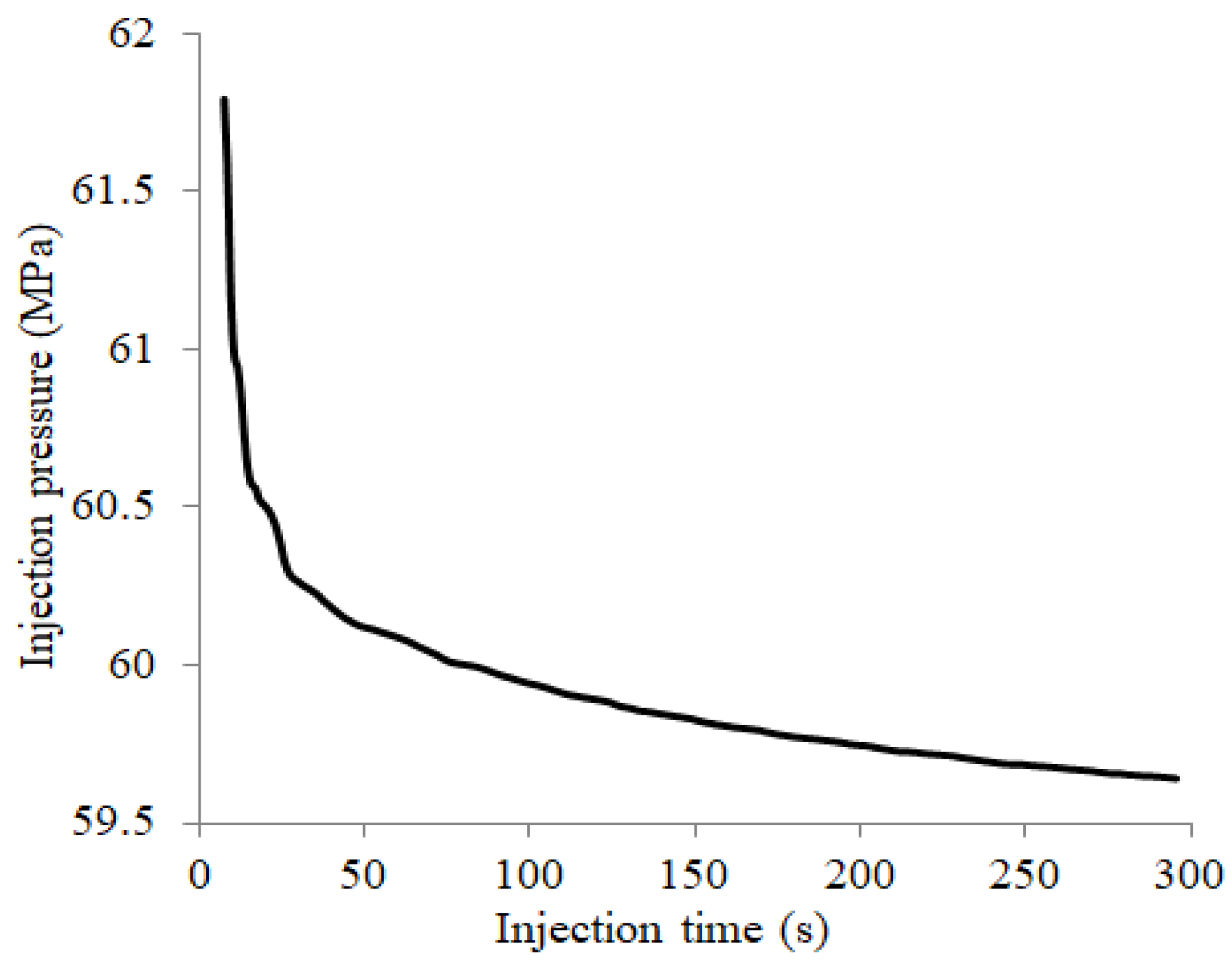
The inlet’s fluid pressure is the highest, while the fluid pressure at the fracture tip is the lowest. The injection pressure declines rapidly in the beginning and then gradually declines later. The final injection pressure tends to the original minimum horizontal stress.

(3)

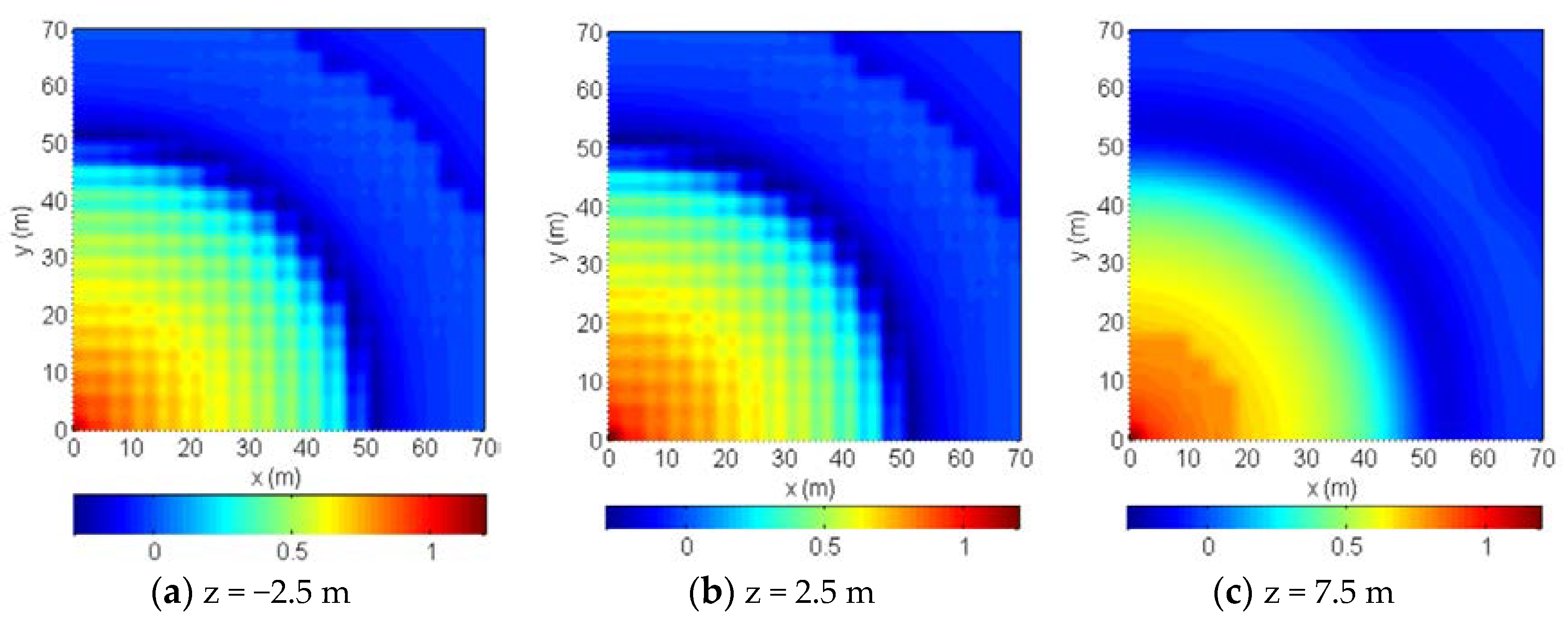
The S_zz in the middle area is much greater than the original minimum horizontal stress, indicating strong compression along the z-axis. In the area far from the horizontal well, S_zz is less than the original minimum horizontal stress, indicating tension along the z-axis induced by the opening fracture. Due to the stress interaction, the interior fractures suffer strong compressive stress, and their propagations are strongly restrained.

(4)

The horizontal stress contrast in the middle area declines after the hydraulic fracturing process. The horizontal stress contrast in the far-field increases after the hydraulic fracturing process. The area close to the wellbore is more likely to include a complex fracture network after the intensive-stage fracturing process.

(5)

Only increasing the perforation cluster number in each stage cannot improve the fracture geometry equilibrium in the intensive-stage fracturing. In this study, site 5-cluster perforation is the best choice for improving the stimulation efficiency. To improve the fracture geometry equilibrium, it is suggested to design more perforation numbers in each perforation cluster and ensure that both the perforation number and diameter in the interior perforation cluster are greater than those of the exterior ones.

References

1. Adachi, J.; Siebrits, E.; Peirce, A.; Desroches, J. Computer simulation of hydraulic fractures. Int. J. Rock Mech. Min. Sci. 2006, 44, 39–757. [Google Scholar] [CrossRef]
2. Castonguay, S.T.; Mear, M.E.; Dean, R.H.; Schmidt, J.H. Predictions of the growth of multiple interacting hydraulic fractures in three dimensions. In Proceedings of the SPE Annual Technical Conference and Exhibition, New Orleans, LA, USA, 30 September–2 October 2013. [Google Scholar]
3. Chan, H.C.M.; Li, V.; Einstein, H.H. A hybridized displacement discontinuity and indirect boundary element method to model fracture propagation. Int. J. Fract. 1990, 45, 263–282. [Google Scholar] [CrossRef]
4. Chen, M.; Zhang, S.; Xu, Y.; Ma, X.; Zou, Y. A numerical method for simulating planar 3D multi-fracture propagation in multi-stage fracturing of horizontal well. Pet. Explor. Dev. 2020, 47, 163–174. [Google Scholar] [CrossRef]
5. Chen, X.; Li, Y.; Zhao, J.; Xu, W.; Fu, D. Numerical investigation for simultaneous growth of hydraulic fractures in multiple horizontal wells. J. Nat. Gas Sci. Eng. 2018, 51, 44–52. [Google Scholar] [CrossRef]
6. Cheng, C.; Bunger, A.P.; Peirce, A.P. Optimal Perforation Location and Limited entry design for Promoting Simultaneous Growth of Multiple Hydraulic Fractures. SPE J. 2016, 21, 145–159. [Google Scholar]
7. Cheng, W.; Jiang, G.; Jin, Y. Numerical simulation on fracture path and nonlinear closure for simultaneous and sequential fracturing in a horizontal Well. Comput. Geotech. 2017, 88, 242–255. [Google Scholar] [CrossRef]
8. Cheng, W.; Jiang, G.; Tian, H.; Zhu, Q. Numerical investigations of the fracture geometry and fluid distribution of multistage consecutive and alternative fracturing in a horizontal well. Comput. Geotech. 2017, 92, 41–56. [Google Scholar] [CrossRef]
9. Cheng, W.; Jiang, G.; Xie, J.; Wei, Z.; Zhou, Z.; Li, X. A simulation study comparing the Texas two-step and the multistage consecutive fracturing method. Pet. Sci. 2019, 16, 1121–1133. [Google Scholar] [CrossRef] [Green Version]
10. Dontsov, E.V.; Suarez-Rivera, R. Propagation of multiple hydraulic fractures in different regimes. Int. J. Rock Mech. Min. Sci. 2020, 128, 104270. [Google Scholar] [CrossRef]
11. Dontsov, E.V.; Peirce, A.P. A multiscale implicit level set algorithm (ILSA) to model hydraulic fracture propagation incorporating combined viscous, toughness, and leak-off asymptotics. Comput. Methods Appl. Mech. Eng. 2017, 313, 53–84. [Google Scholar] [CrossRef]
12. Gunaydin, D.; Peirce, A.P.; Bunger, A. Laboratory experiments contrasting growth of uniformly and nonuniformly-spaced hydraulic fractures. J. Geophys. Res. Solid Earth 2021, 126. [Google Scholar] [CrossRef]
13. He, J.; Zhang, Z.; Li, X. Numerical analysis on the formation of fracture network during the hydraulic fracturing of shale with pre-existing fractures. Energies 2017, 10, 736. [Google Scholar] [CrossRef] [Green Version]
14. Long, G.; Xu, G. The effects of perforation erosion on practical hydraulic-fracturing applications. SPE J. 2017, 22, 645–659. [Google Scholar] [CrossRef]
15. Li, Y.; Deng, J.; Liu, W.; Feng, Y.; Cao, W.; Wang, P.; Hou, Y. Numerical simulation of limited-entry multi-cluster fracturing in horizontal well. J. Pet. Sci. Eng. 2017, 152, 443–455. [Google Scholar] [CrossRef]
16. Kumar, D.; Ghassemi, A. A three-dimensional analysis of simultaneous and sequential fracturing of horizontal wells. J. Pet. Sci. Eng. 2016, 146, 1006–1025. [Google Scholar] [CrossRef]
17. Nguyen, V.P.; Lian, H.; Rabczuk, T.; Bordas, S. Modelling hydraulic fractures in porous media using flow cohesive interface elements. Eng. Geol. 2017, 225, 68–82. [Google Scholar] [CrossRef]
18. Olson, J.E.; Pollard, D.D. Inferring paleostresses from natural fracture patterns: A new method. Geology 1989, 17, 345–348. [Google Scholar] [CrossRef]
19. Peirce, A.P.; Bunger, A. Interference fracturing: Nonuniform distributions of perforation clusters that promote simultaneous growth of multiple hydraulic fractures. SPE J. 2015, 20, 384–395. [Google Scholar] [CrossRef] [Green Version]
20. Rabczuk, T.; Belytschko, T. Cracking particles: A simplified meshfree method for arbitrary evolving cracks. Int. J. Numer. Methods Eng. 2004, 61, 2316–2343. [Google Scholar] [CrossRef]
21. Ren, H.; Zhuang, X.; Cai, Y.; Rabczuk, T. Dual-horizon peridynamics. Int. J. Numer. Methods Eng. 2016, 108, 1451–1476. [Google Scholar]
22. Ren, H.; Zhuang, X.; Rabczuk, T. Dual-horizon peridynamics: A stable solution to varying horizons. Comput. Methods Appl. Mech. Eng. 2017, 318, 762–782. [Google Scholar] [CrossRef] [Green Version]
23. Sesetty, V.; Ghassemi, A. A numerical study of sequential and simultaneous hydraulic fracturing in single and multi-lateral horizontal wells. J. Pet. Sci. Eng. 2015, 132, 65–76. [Google Scholar] [CrossRef]
24. Shen, B.; Shi, J. A numerical scheme of coupling of fluid flow with three-dimensional. Eng. Anal. Bound. Elem. 2019, 106, 243–251. [Google Scholar] [CrossRef]
25. Shou, K.J.; Siebrits, E.; Crouch, S.L. A higher order displacement discontinuity method for three-dimensional elastostatic problems. Int. J. Roch Mech. Min. Sci. 1997, 34, 317–322. [Google Scholar] [CrossRef]
26. Tang, H.; Winterfeld, P.H.; Wu, Y.; Huang, Z.; Di, Y.; Pan, Z.; Zhang, J. Integrated simulation of multi-stage hydraulic fracturing in unconventional reservoirs. J. Nat. Gas Sci. Eng. 2018, 51, 44–52. [Google Scholar] [CrossRef]
27. Tang, H.; Wang, S.; Zhang, R.; Li, S.; Zhang, L.; Wu, Y. Analysis of stress interference among multiple hydraulic fractures using a fully three-dimensional displacement discontinuity method. J. Pet. Sci. Eng. 2019, 179, 378–393. [Google Scholar] [CrossRef]
28. Wang, W.; Dahi Taleghani, A. Simulating multizone fracturing in vertical wells. J. Energy Resour. Technol. 2014, 136, 124–136. [Google Scholar] [CrossRef]
29. Wu, K.; Olson, J.E. Simultaneous multifracture treatments: Fully coupled fluid flow and fracture mechanics for horizontal wells. SPE J. 2015, 20, 334–346. [Google Scholar] [CrossRef]
30. Wu, K.; Olson, J.E. A simplified three-dimensional displacement discontinuity method for multiple fracture simulations. Int. J. Fract. 2015, 193, 191–204. [Google Scholar] [CrossRef]
31. Wu, K.; Olson, J.E.; Balhoff, M.; Yu, W. Numerical Analysis for Promoting Uniform Development of Simultaneous Multiple-Fracture Propagation in Horizontal Wells. SPE Prod. Oper. 2016, 32, 155–167. [Google Scholar]
32. Wu, R.; Bunger, A.P.; Jeffrey, R.G.; Siebrits, E. A comparison of numerical and experimental results of hydraulic fracture growth into a zone of lower confining stress. In Proceedings of the 42nd U.S. Rock Mechanics Symposium, San Francisco, CA, USA, 29 June–2 July 2008. [Google Scholar]
33. Vahab, M.; Khalili, N. X-FEM modeling of multizone hydraulic fracturing treatments within saturated porous media. Rock Mech. Rock Eng. 2018, 51, 3219–3239. [Google Scholar] [CrossRef]
34. Xu, G. Interaction of multiple non-planar hydraulic fractures in horizontal wells. In Proceedings of the International Petroleum Technology Conference, Beijing, China, 26–28 March 2013. [Google Scholar]
35. Yew, C.H.; Weng, X. Mechanics of Hydraulic Fracturing [M]; Elsevier: Amsterdam, The Netherlands, 2015. [Google Scholar]
36. Zeng, Q.; Liu, W.; Yao, J. Numerical modeling of multiple fractures propagation in anisotropic formation. J. Nat. Gas Sci. Eng. 2018, 53, 337–346. [Google Scholar] [CrossRef]
37. Zhang, F.; Dontsov, E. Modeling hydraulic fracture propagation and proppant transport in a two-layer formation with stress drop. Eng. Fract. Mech. 2018, 199, 705–720. [Google Scholar] [CrossRef]
38. Zhang, Z.; Li, X.; Yuan, W.; He, J.; Li, G.; Wu, Y. Numerical analysis on the optimization of hydraulic fracture networks. Energies 2015, 8, 12061–12079. [Google Scholar] [CrossRef]
39. Zheng, Y.; Fan, Y.; Yong, R.; Zhou, X. A new fracturing technology of intensive stage+high-intensity proppant injection for shale gas reservoir. Nat. Gas Ind. 2020, 7, 292–297. [Google Scholar] [CrossRef]
40. Zeller, S.S.; Pollard, D.D. Boundary conditions for rock fracture analysis using the boundary element method. J. Geophys. Res. 1992, 97, 1991–1997. [Google Scholar] [CrossRef]
41. Zhuang, X.; Zhou, S.; Sheng, M.; Li, G. On the hydraulic fracturing in naturally-layered porous media using the phase field method. Eng. Geol. 2020, 266, 105306. [Google Scholar] [CrossRef]
42. Zeng, Q.; Yao, J.; Shao, J. An extended finite element solution for hydraulic fracturing with thermo-hydro-elastic–plastic coupling. Comput. Methods Appl. Mech. Eng. 2020, 364, 112967. [Google Scholar] [CrossRef]
43. Zhang, F.; Wang, X.; Tang, M.; Du, X.; Xu, C.; Tang, J.; Damjanac, B. Numerical investigation on hydraulic fracturing of extrenme limited entry perforating in plug-and-perforation completion of shale oil reservoir in Changqing oilfield, China. Rock Mech. Rock Eng. 2021, 02, 1–18. [Google Scholar]
Figure 1. Sketch of intensive fracturing.
Energies 14 02393 g001
Figure 2. Rectangular fracture mesh.
Energies 14 02393 g002
Figure 3. Sketch of fracture elements.
Energies 14 02393 g003
Figure 4. Workflow of the fluid–solid coupling method.
Energies 14 02393 g004
Figure 5. Comparison of the analytical and numerical solutions.
Energies 14 02393 g005
Figure 6. Hydraulic fracture width distribution.
Energies 14 02393 g006
Figure 7. Width of the fracture center versus the injection time.
Energies 14 02393 g007
Figure 8. Fluid pressure distribution inside the fracture.
Energies 14 02393 g008
Figure 9. Injection pressure at the wellbore inlet.
Energies 14 02393 g009
Figure 10. Szz (MPa) distribution on the x–z plane.
Energies 14 02393 g010
Figure 11. Δ S zz (MPa) distribution on 1/4 of the x–y plane.
Energies 14 02393 g011
Figure 12. Sxx distribution on the x–z plane.
Energies 14 02393 g012
Figure 13. Δ S x x (MPa) distribution on 1/4 of the x–y plane.
Energies 14 02393 g013
Figure 14. KHh distribution on the x–z plane.
Energies 14 02393 g014
Figure 15. Fracture area versus the perforation cluster number.
Energies 14 02393 g015
Figure 16. Centric width of fracture versus the perforation cluster number.
Energies 14 02393 g016