Analysis of the Influence of Motors Installed in Passenger Car Wheels on the Torsion Beam of the Rear Axle Suspension

Abstract

The influence of mounting motors in wheels’ hubs and flexibility of the twist beam rear suspension on their dynamics and strength is presented in the paper. The international roughness indicator (IRI) is applied to assess the overcoming of road unevenness. This indicator is a combination of a shape of the road unevenness and of overcoming velocity. The movement of a wheel’s axis during obstacles overcoming is described. For the needs of the dynamics analysis, the mathematical model of the rear suspension system with embedded motors is developed using the MSC.Adams-ANSYS interface. The discrete model of the twist beam is prepared in the ANSYS software, which is used in the next step to construct the dynamics model of the rear suspension system using the MSC.Adams program. The vertical components of displacement and acceleration of the wheel’s centre, forces in the suspension’s springs and dampers, as well as forces in the joints are analyzed. The analysis of the suspension beam’s stress during the road unevenness overcoming is also carried out.

1. Introduction

In the era of growing market share in hybrid and electric cars, it is worth considering how mounting motors in a vehicle’s wheels affects its movement and the strength of the suspension components. The application of such driving systems change many factors, which can affect vehicles’ dynamics, such as safety, ease of steering, comfort and the durability of the suspension components. Due to a very wide range of issues, authors focus only on the assessment of a vehicle’s behaviour during road unevenness overcoming. The analysis is carried out for motors placed in the wheels of the rear axle of a car with a semi-dependent suspension and a twist beam. Such suspension consists of two trailing arms connected by a twist beam. In a semi-dependent suspension, the vertical motion of the wheels slightly influence each other. A twist beam is located in the front of a wheel axle and is subjected to torsional forces, acting as a stabilizer. This solution does not generate high production and operating costs. It also causes, under the action of lateral forces, the wheels to tilt only slightly, which improves the grip of the car’s wheels. Usually, coil springs or a torsion bar are elastic elements in this type of suspension.

Incorrect operation of a suspension can cause the premature wear of tires, suspension joints, steering system, wheel’s bearings, and body mounting elements, as well as increase the braking distance.

The use of drive motors in wheels, despite the significant simplification of the drive system, is not a common solution, because the required driving force acting at the contact point of the wheel with the road results from the values of torque generated by the motor and the radius of the wheel. Car wheel diameters are usually proportional to the dimensions of the vehicle. The diameter of the wheel rim, in which the electric motor is mounted, cannot be too large either. Additionally, the required drive torque is relatively high and depends on the weight of the vehicle. Obtaining such torque requires large dimensions of the motor. Placing the motors in the wheels deteriorates the ratio of sprung to unsprung masses, which reduces driving comfort.

2. Literature Review and Paper Contributions

Installing motors in the rear wheels of a vehicle increases the weight of a suspension and its moments of inertia (this applies to the rotational motion of wheels and the vertical movement of a suspension) [1,2,3,4]. It also increases the mass of unsprung elements and generates larger loads acting on the suspension’s elements.

In the literature, one can find few studies in which the analysis of the impact of mounting motors in vehicle wheels on comfort, vehicle properties, and durability of rear suspension components is comprehensively treated [5,6]. The most common are quarter rear suspension models, in which a simplified model of interaction between the suspension and the wheel is used, and unevenness on the road is modeled by kinematic inputs.

In the paper [7], X. Jiao and M. Bienvenu used the IRI (international roughness indicator) to assess the road surface condition and its impact on fuel consumption on motorway sections. It was also used to determine the rolling resistance coefficient of the vehicle. The report of the Iowa State University [8] investigated the interaction between the vehicle and the bridge during overcoming the unevenness on the bridge, which results in the dynamic loads acting between the vehicle and the bridge. The unevenness overcoming issues was described by the authors in previous works [9,10].

In this study, the IRI factor is used to evaluate the obtained results. This factor allows to refer the road unevenness to the vehicle velocity. The mechanics of the road unevenness overcoming is presented. It was proven that mounting motors in the wheels reduces the comfort of single road unevenness overcoming. A simulation model of the rear suspension with the compound twist beam axles (a typical solution used in small vehicles and the test vehicle) is built to carry out a more detailed analysis. The model is prepared in the MSC.Adams system (MSC Software, Newport Beach, CA, USA) and the obtained simulation results are used to conduct a strength analysis of the twist-beam axle, using the ANSYS system (ANSYS, Canonsburg, PA, USA). It allowed to determine the areas of stress concentration and compare them for a vehicle with motors mounted in the vehicle’s wheels and without them.

3. Road Unevenness and Their Assessment

The universal testing procedure was developed at the request of the World Bank to harmonize measuring methods and qualify road surfaces. According to this procedure, the international roughness index ($IRI$) was introduced, which combines a description of the road surface damage condition with a safe vehicle’s velocity (Figure 1). The value of this indicator depends on the standard of a road. From the computational point of view, the $IRI$ indicator is a ratio of cumulative vertical movements of a body and a wheel to a road traveled by the vehicle during the test, determined on the basis of the analysis of the movement of a body and a wheel in a quarter car model [11,12].

A value of the indicator $IR{I}_i$ for a single unevenness of the road is determined for a single calculation step, and it is equal to the ratio of a deflection speed of a suspension system to an assumed vehicle velocity. In practice, it determines the ratio of a deflection of a suspension system to a road traveled at that time. A surface unevenness index, as an $IRI$ segmental assessment, corresponds to an average value of suspension deflections, which is calculated as the arithmetic mean ${\displaystyle \sum _{i=1}^{n}IR{I}_i}$ for the $n$ measurements. In accordance with the established calculation procedure, the surface unevenness index $IRI$ is determined according to the following relationship

$$IRI=\frac{1}{n}{\displaystyle \sum _{i=1}^{n}IR{I}_i}=\frac{1}{nV}{\displaystyle \underset{0}{\overset{n}{\int }}\left|{\dot{z}}_{b,i}-{\dot{z}}_{w,i}\right|}\mathrm{d}t,$$

(1)

where ${{\dot{z}}_{\alpha }|}_{\alpha \in \left\{b,w\right\}}$ are the vertical displacements and velocities of the body ($b$), wheel ($w$), and velocity (V).

In this work, the authors deal with the problem of changing wheel loads when overcoming single road unevenness.

After preliminary tests, it was found that unfavourable impact is particularly due to road unevenness in the shape of a single depression in a roadway and protuberances, similar to overcoming an obstacle. These are the most common road unevenness types that generate dynamic forces loading the suspension.

During the analysis, the simulation model described below is used. The results of previous analyses of the simpler model are described in [14,15,16]. In these papers, road test results were used to validate the simulation model. The paper presents an analysis of the vehicle motion for different vehicle velocities.

In the first part, an analysis of the suspension movement is performed, and the forces affecting the suspension are determined. In the second part of the paper, the strength analysis of the suspension twist beam during overcoming selected road unevenness is performed. Stresses of the twist beam suspension of the car are analyzed for the system with and without motors mounted in wheels. The modeling of the movement of the wheel axle during overcoming road unevenness is a very important issue [17,18,19].

4. Mechanics of Overcoming Single Road Unevenness

The problem of the wheel axis movement and forces acting on it results from the height and shape of road unevenness, wheel movement velocity, suspension characteristics, and vehicle parameters. During road unevenness overcoming, additional loading forces act on the wheel [17,20,21,22,23]. Loads arising during rectilinear wheel movement and when hitting on the road unevenness are shown in Figure 2. The rolling resistance force $f_{h,0}$ is omitted in Figure 2b,c in order to improve its readability.

The horizontal component of the wheel load force depends on the effective angle of a road plane inclination, vehicle velocity, and shape of the unevenness. As a result of the suspension’s deflection, the wheel is loaded with greater force—an additional force is generated, which loads the wheel $f_n^{*}$, $f_n=f_{n,0}+f_n^{*}$. The reaction force $f_z$ is transmitted entirely by the tire. The tire deflection occurring on the edge of the unevenness largely depends on the effective angle of the road plane, the contact area of the tire with the road unevenness, and its height and shape.

Increasing the overcoming velocity through road unevenness results in a decrease in the relative amplitude, defined as the ratio of the maximum value of the vertical movement amplitude of the vehicle body to the height of the unevenness. As the vehicle velocity increases, the vertical load of the wheel increases due to the inertia of the car body when overcoming road unevenness (Figure 3).

Comparing the wheel movement during overcoming road unevenness to the movement on a flat horizontal road, it can be stated that, apart from forces occurring in the rectilinear motion (rolling resistance force and forces resulting from the movement conditions—driving or braking), it can be noted the following additional forces loading the wheel and suspension:

• Additional vertical force resulting from suspension deflection (the wheel lift and body inertia);
• Horizontal force consisting of

  (a)

  Horizontal resultant force component $f_h$ resulting from the wheel load with force $f_{n,0}$ during overcoming road unevenness;

  (b)

  Component of additional loading force $f_n^{*}$ resulting from the shape of the road unevenness and driving velocity.

To model the movement of the wheel axle, the model proposed by Zegelaar using the two-point beam technique [17,18,20] is used. The possibility of using the smoothing properties of tires, described in [19], is also analyzed. Ultimately, the model of the tire’s contact points of the road and unevenness is used in the analysis.

In the model proposed by Zegelaar [20], the wheel rolls on the road unevenness; however, the movement of the wheel axis is determined using a curve (sinusoid) on which a beam of a certain length moves. The beginning and the end of the beam move along a curve, and its center is determined by the trajectory of the wheel axis. In the case of overcoming road unevenness of a rectangular shape, the procedure for determining the movement of the wheel axis is supplemented with a section connecting the entry to and exit from the unevenness. The diagram for determining the wheel axis motion is shown in Figure 4.

The methodology presented in [19] takes into account the smoothing properties of tires, and uses the fact that the tire, in the area of the contact patch with the road, averages the height of road unevenness and filters the spectrum of road unevenness in this area. This allows using the model of the point cooperation of the tire with the road

$$S_{df}(\Omega )=H^2{S}_d(\Omega ),$$

(2)

where $S_d(\Omega ), {\mathrm{m}}^3{\mathrm{rad}}^{-1}$ is the power spectral density of a single longitudinal trace, $\Omega =2\pi /L, {\mathrm{radm}}^{-1}$ is the circular road frequency, $L, \mathrm{m}$ is the wavelength of road unevenness, and $H$ is the filter that allows for point cooperation of the wheel model with the road.

The analysis of the contact conditions of the wheel points with the road surface and unevenness is described below.

5. Analysis of the Dynamic’s Load of the Rear Axle

Based on the tests described in [22], the results obtained for the vehicle with and without motors mounted in the rear wheels are compared. The $IRI$ indicator calculated for a single road unevenness is applied to assess the impact of mounting motors in the wheels on the vehicle motion. The values of this indicator are determined based on the vertical movement of the body and the wheel during the rectangular unevenness overcoming. The $IRI$ indicators obtained from road tests are compared with those obtained from simulations.

Table 1. List of $IRI$ indicators determined from the road tests ($\upsilon =12.5 {\mathrm{kmh}}^{-1}$).

Vehicle	Without Load	With Load
Unevenness U
without motors in wheels	17.35	17.88
with motors in wheels	19.87	20.24
Unevenness E
without motors in wheels	17.46	17.41
with motors in wheels	18.92	20.85

Where U—unevenness in the form of depression, E—unevenness in the form of protuberant.

contains values of the $IRI$ indicator for individual overcoming tests with the velocity of $~12 {\mathrm{kmh}}^{-1}$ for the vehicle without the load (with driver only) and with the load (driver and passengers).

Based on the results obtained and Equation (1), the maximum overcoming velocity for an individual unevenness can be determined. It means that comfortable overcoming of a short single unevenness requires a reduction in vehicle velocity. Comfortable overcoming of a rectangular obstacle requires reducing the velocity to $~30 {\mathrm{kmh}}^{-1}$ when a vehicle is unloaded. Increasing the vehicle load allows to overcome unevenness with a slightly higher velocity. The installation of motors in the wheels of a vehicle increases values of the $IRI$ coefficients by ~10%. Overcoming road unevenness of a larger length leads to separation of the unevenness entry and exit phases, so it is possible to overcome the obstacle at higher velocities.

Overcoming the obstacle in the shape of a step causes the wheel, in the middle phase of overcoming, to not contact the obstacle bottom but rest on its wall. Increasing the velocity shifts the lowest contact point toward the step wall in the direction of the vehicle movement. This condition causes a rapid change in the velocity direction of the wheel axis, which can cause an occurrence of greater accelerations and thus, the vertical velocity of the wheel axis. The vehicle loads generate smaller amplitudes of the wheel vibrations. Increasing the overcoming velocity can cause a decrease in the amplitude of the body vibrations, which are caused by the body’s inertia, and increase the horizontal component of the reaction forces acting on the wheel [9].

6. Dynamics Model of the Rear Axle Twist Beam Suspension

The MSC.Adams package is used to elaborate the dynamics model of the rear suspension when overcoming an obstacle. This model was validated in earlier works of the authors; however, the flexibility of the suspension beam was not taken into account [14,15]. The numerical model of the rear suspension with the flexible beam is prepared using the interface MSC.Adams and ANSYS packages. The scheme of such cooperation is shown in Figure 5. The interaction between the flexible beam and the remaining suspension elements is implemented through interface points. The simulation in the MSC.Adams package allows to determine the stress distribution and the time stamps for which the stresses are the largest, but this assessment is rough. More accurate stress distribution over time can be calculated in the ANSYS package after loading the forces acting on the interface points, calculated in the MSC.Adams package.

According to the scheme shown in Figure 5, the multibody model of the rear suspension system is modeled using the MSC.Adams package. Unlike the models presented in earlier works [14,15,16], the method of the interconnection of the beam with the body is modified. The previous model assumed that suspension during overcoming an obstacle rotates around the axis of the spherical joint formed between the suspension beam and the body. While such assumptions are acceptable in the case when the suspension’s beam is treated as rigid, in the case of the flexible beam, it can lead to excessive stresses that do not exist in the real system. In order to obtain numerical results more consistent with those measured during road tests, a sliding joint, which takes into account the vertical displacements of the beam during overcoming of the obstacle, is introduced to the system. In addition, the rigid beam is introduced to take into account the interaction between suspension springs (Figure 6).

In the calculations, it is assumed that the suspension’s beam is made of the AISI 4130 steel. This steel, also known as chromium or chromium–molybdenum steel alloy, has admixtures of chromium ($0.8÷1.1\%$) and molybdenum ($0.15÷0.25\%$), which are used as reinforcing agents.

It exhibits the following mechanical properties:

• Density—$7850{ \mathrm{kgm}}^{-3}$;
• Hardness—217 (Brinell scale)–95 (Rockwell B);
• Ultimate tensile strength—$540 \mathrm{MPa}$;
• Yield tensile strength—$460 \mathrm{MPa}$;
• Modulus of elasticity—$205 \mathrm{GPa}$;
• Machinability—72% (in annealed state).

Other advantages of this material include high plasticity, good weldability and workability.

The numerical model of the flexible beam is modeled using the ANSYS package. The suspension beam is divided into 231,039 solid and 7380 beam finite elements (Figure 7). Due to a large number of irregular and curved surfaces, making a finite element mesh is a complex task, and it requires many iterations to achieve an appropriate quality of the discrete model.

Loads acting on the beam are introduced by the so-called interface points, i.e., points where forces and torques calculated in the MSC.Adams are applied (Figure 8). These points are determined in the ANSYS package and then exported with the discrete beam model to the MSC.Adams package. In the considered model, it is assumed that the interface points are located in places where the suspension beam is joined with other parts of the rear suspension system.

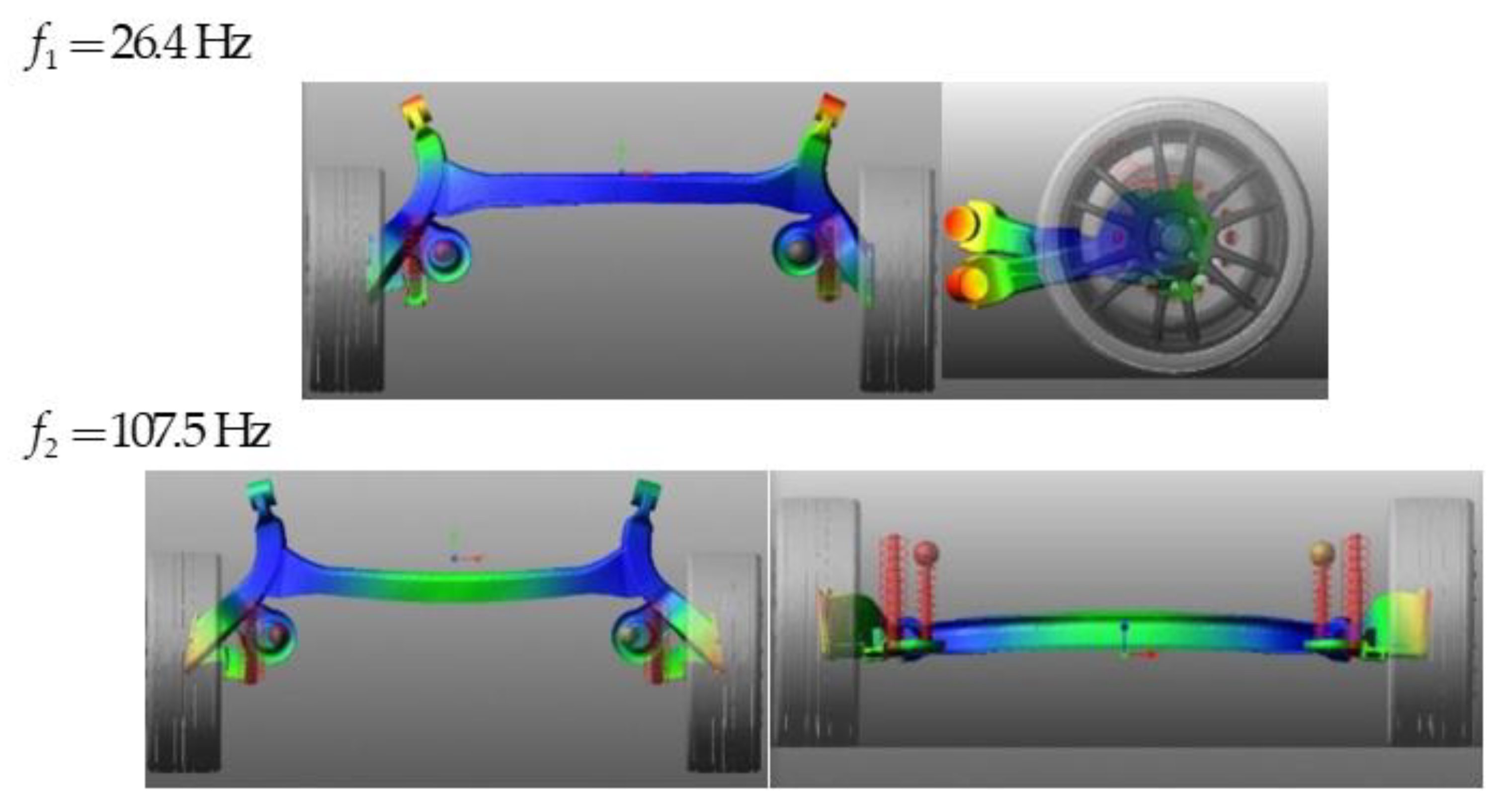
It is assumed that the exported suspension beam model contains 48 natural frequencies. The number of frequencies is limited to those which are the most important when determining the dynamic response of the system. Figure 9 shows the first two frequencies of free vibrations and the corresponding forms of vibrations. Analyzing the presented forms of vibration, it can be seen that the deformations associated with bending and torsion are dominant for the analyzed frequencies.

The results of the simulation of the wheel overcoming obstacles are presented in the further part of the paper. The purpose of these simulations is to determine the effect of additional unsprung masses from motors built into wheel hubs on the dynamic response of the suspension. It is assumed that the wheels overcome obstacles at speeds of 30, 60 and $90 {\mathrm{kmh}}^{-1}$.

The simulations analyze the dynamic response of the rear suspension system when overcoming obstacles, shown in Figure 10. These obstacles are a fairly common case of unevenness occurred on roads.

The selected time histories obtained for the suspension with the rigid beam during overcoming the U-type obstacle are presented in Figure 11. In the simulations, the effect of additional unsprung masses from motors built into the wheels on the dynamics is additionally analyzed.

Analyzing the presented results, it can be seen that the introduction of additional masses does not have a major impact on the displacement of the center of the wheel and the forces acting on the suspension spring. The influence of these masses is visible in the course of forces acting in the shock absorber and in the spherical joint, where the beam joins the car’s body. Similar analyses are made for the system with the flexible beam, and their results are presented in Figure 12.

Analyzing the results obtained, it can be seen that the introduction of additional masses, resulting from the assembly of the motors in wheels, has no major impact on the dynamic response of the suspension. Comparing the results from Figure 11 with the results from Figure 12, it can be seen that taking into account the suspension beam’s flexibility leads to a slight increase in the amplitudes of displacement and acceleration of the wheel’s center as well as forces acting in the suspension spring and damper. Moreover, in the model with the flexible beam, additional oscillations appear just after obstacle overcoming. Particularly noteworthy is the force acting in the spherical joints. It can be seen that in the case of the flexible beam, these forces are greater than those occurring in the model with the rigid beam. In addition, it can be seen that as the overcoming obstacle velocity increases, the loads acting on the system are smaller.

In Figure 13 and Figure 14, selected time courses obtained for the E type obstacle are compared. The influence of the additional masses from the motors’ built-in wheels and the suspension beam’s flexibility on the response of the rear suspension system are analyzed in the presented simulations results.

Analyzing the courses presented, it can be seen that the response of the system obtained for the obstacle overcoming velocities $60 {\mathrm{kmh}}^{-1}$ and $90 {\mathrm{kmh}}^{-1}$ is very similar. For velocity $30 {\mathrm{kmh}}^{-1}$, the forces acting in the rear suspension system are significantly smaller. Examining the accelerations of the wheel’s center for the system with the rigid beam and without motors in the wheels obtained for overcoming velocity equal to $90 {\mathrm{kmh}}^{-1}$, it can be seen that after entering the obstacle, the acceleration increases rapidly to around $80 \mathrm{m} {\mathrm{s}}^{-2}$. The time courses of forces acting in the spherical joint connecting the suspension beam with the body are interesting. In the case when the beam is treated as rigid, there is observed a peak for the force in the spherical joint after overcoming the obstacle. After this peak, the force decreases to the level occurring before entering the obstacle. Forces acting in the spherical joint look different in the model with the flexible beam. In this model, the forces increase rapidly during overcoming the obstacle, after which there are damped oscillations with relatively large amplitudes.

Figure 15 shows the distribution of reduced stress obtained from the solution of the static task for the suspension system with and without motors in wheels.

Analyzing the results shown in Figure 15, it can be seen that the reduced stresses in the suspension beam do not exceed 43 MPa. In the analysis, stresses above 43 MPa are rejected. They result from the simplifications used in modeling stress concentration areas (sharp edges, places of connection of mounting plates with the suspension beam) and from the applied method of modeling joints (forces from joints are transferred to the system through interface points).

Figure 16, Figure 17 and Figure 18 show the results of the strength calculations in the form of contour plots of the reduced stresses before and during overcoming the obstacle, obtained at the time when the reduced stresses reach their highest values.

Additionally, the values of the maximum reduced stresses of the system with and without motors obtained for both analyzed obstacles are calculated in order to assess the impact of the obstacle overcoming velocity on the suspension beam’s strength (Figure 19).

Analyzing the results obtained, the following conclusions can be drawn:

• The highest stress concentration are located in places where the spring and damper are assembled to the beam.
• In the case of obstacle E, it can be seen that for a system without motors, the maximum reduced stresses of the suspension beam are greater than those occurring in the system with the motors built into the wheels (Figure 19). In addition, as the obstacle overcoming velocity increases, the difference between the stresses obtained for the system with and without motors in wheels increases. For velocity $\upsilon =90 {\mathrm{kmh}}^{-1}$, the difference is about 100 MPa, and the stresses occurring in the beam are close to the tensile strength (Figure 19).
• In the case of obstacle U, it can be noticed that the maximum reduced stresses decrease as the obstacle overcoming velocity increases. For $\upsilon =90 {\mathrm{kmh}}^{-1}$ the maximum reduced stresses are three times smaller than those obtained for velocity $\upsilon =30 {\mathrm{kmh}}^{-1}$.

7. Conclusions

The first part of the paper presents the IRI indicator, combining the assessment of road surface unevenness with driving speed. This indicator was used to assess unevenness overcoming during the road tests. The movement of the wheel axis during single road unevenness overcoming was described. In the further part of the paper, the road unevenness was used as enforcement during the simulation of the dynamics of the rear suspension system. The paper presents a computational model of the rear suspension system for dynamics analysis. This model enables stress analysis of the suspension beam during obstacle overcoming for two variants: with motors built into wheel hubs and without motors. The finite element method implemented in the ANSYS commercial package was used to model the flexibility of the beam of the semi-dependent rear suspension. Thanks to the use of the MSC.Adams-ANSYS program interface, it was possible to analyze the beam strength for loads acting during unevenness overcoming and to take into account the couplings occurring between the deformable beam and other suspension elements. The results of the numerical simulations allow to formulate the following conclusions:

• Obstacles that were used during the dynamics analysis can be classified as “rough unpaved road” in Figure 1. This means that traveling at a velocity greater than $\upsilon =80 {\mathrm{kmh}}^{-1}$ can lead to significant damage to the suspension. This is also confirmed by the stress values shown in Figure 19.
• In the case of the obstacle E overcoming, the reduced stresses increase with the travel velocity, and for velocity above $\upsilon =80 {\mathrm{kmh}}^{-1}$, they can exceed the allowable values. Slightly different conclusions can be formulated in the case of the U-type obstacle. For this obstacle, the reduced stresses decrease with the travel velocity. This is due to the way the shock absorber works and the wheel inertia—at higher speeds, the wheel “jumps” over a U-type obstacle.
• The simulation results show that greater dynamic forces and stresses in the beam occur during overcoming unevenness in the form of a cavity in the roadway than protuberances. In the case of a cavity, the highest loads occur at lower speeds ($\upsilon =30 {\mathrm{kmh}}^{-1}$ in the analyzed case). At higher speeds, the wheel “jumps” through this cavity, as a result of which the forces and stresses are much smaller.
• It is also noticeable that smaller dynamic forces and stresses occur when the motors are built into the wheel hubs. This is due to increased wheel inertia.
• The fatigue strength of the suspension beam was not analyzed; however, it can be assumed that the final solution will require its local reinforcement.
• Experimental verification of the obtained results is planned in the future.