
AIS-Based Estimation of Hydrogen Demand and Self-Sufficient Fuel Supply Systems for RoPax Ferries


Abstract
:1. Introduction
2. Preliminaries
2.1. Energy Use Prediction
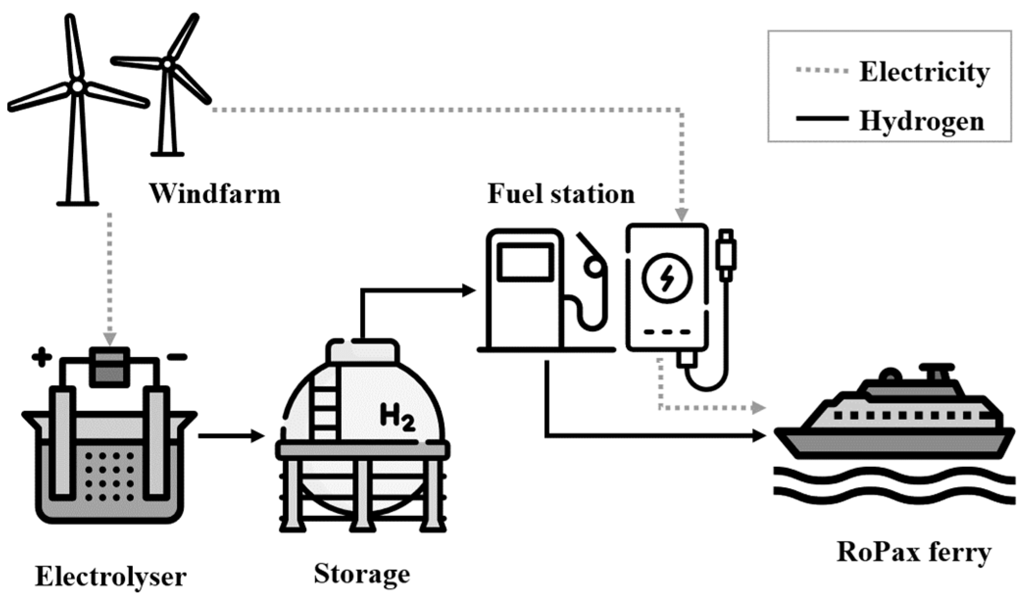
2.2. Energy Supply with Hydrogen as Energy Carrier
3. Materials and Methods
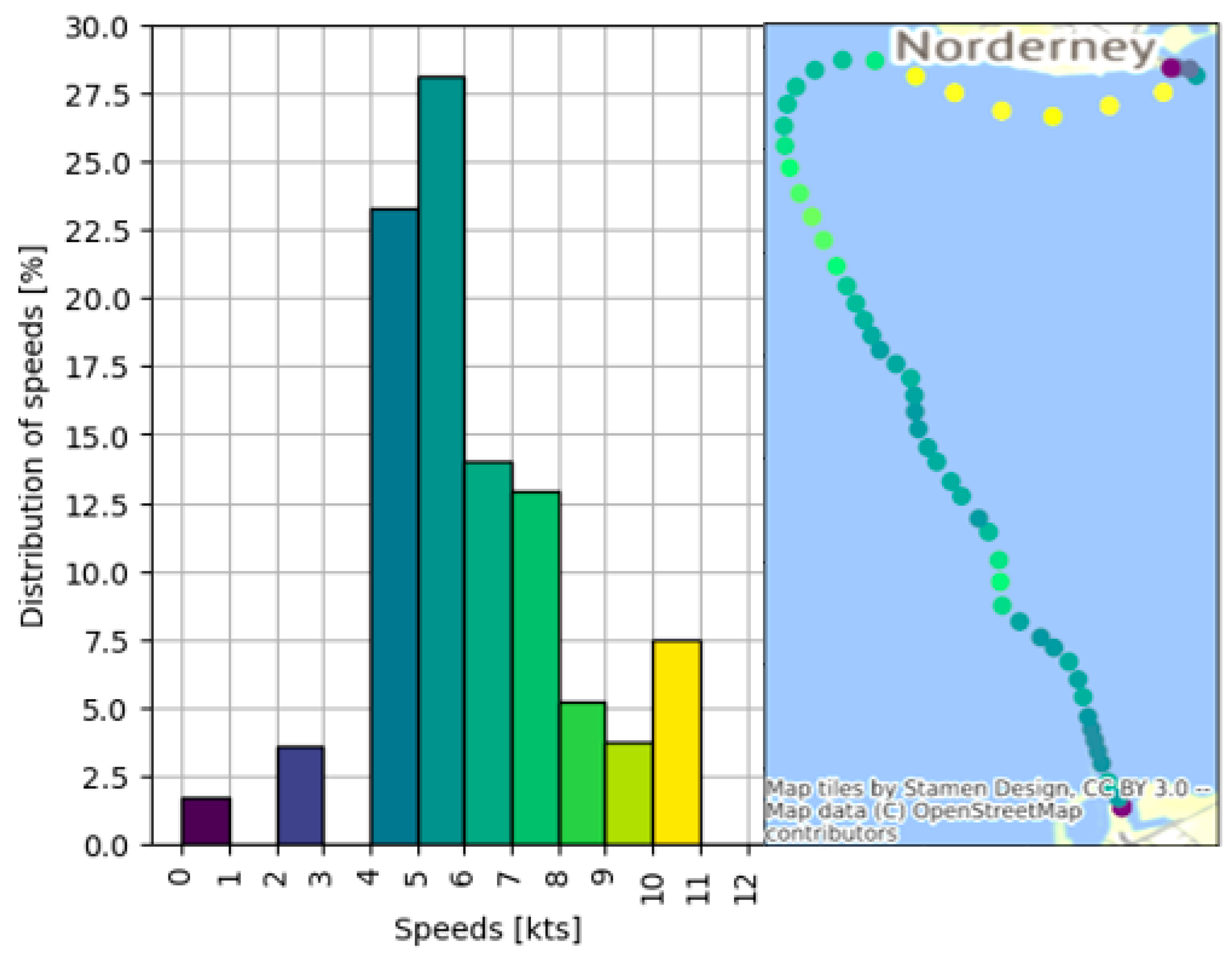
3.1. Operational Analysis
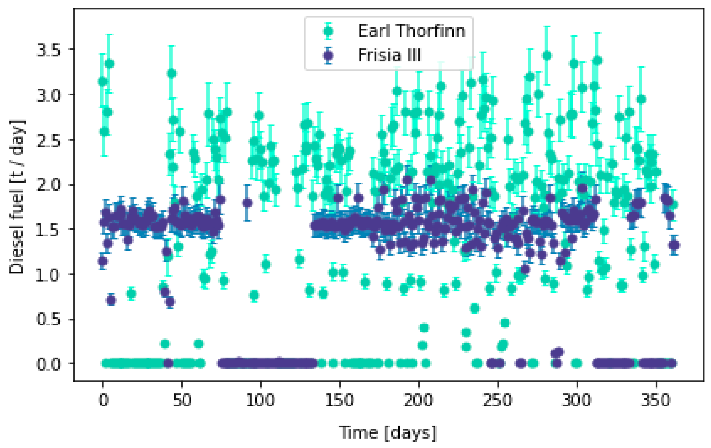
3.2. Energy Use Prediction
3.2.1. Ship Technical Parameters
3.2.2. Speed Penalties
3.2.3. Main Engine Power
3.2.4. Auxiliary Engine Power
3.2.5. Total Fuel Consumption and Emissions
3.3. Low-Carbon Technology Transition
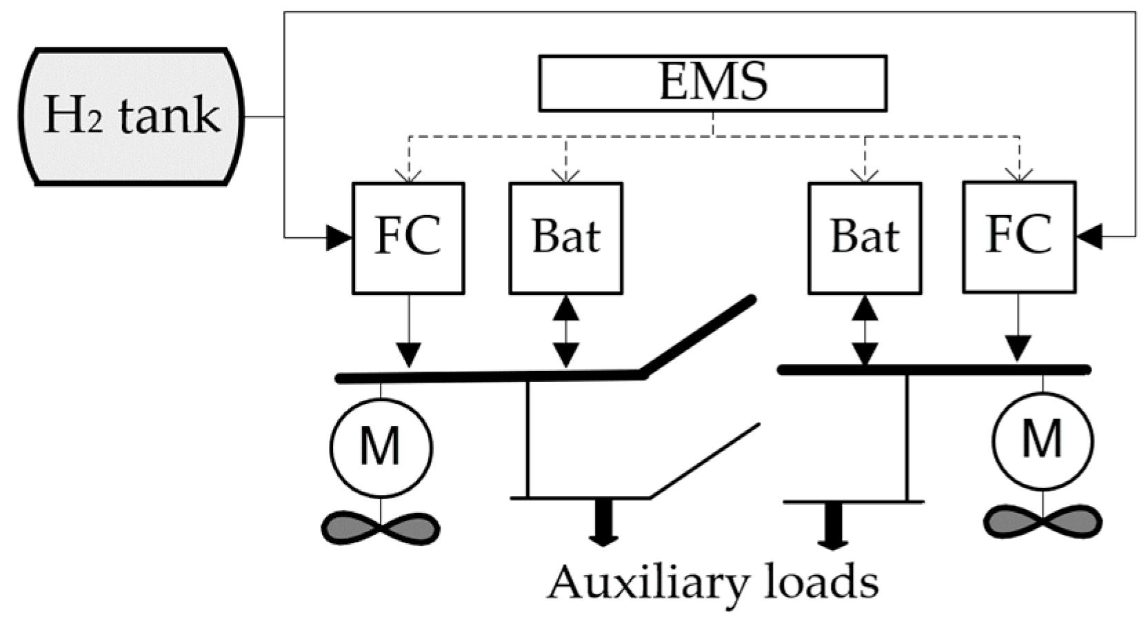
3.3.1. Fuel Cell Hybrid Propulsion System
3.3.2. Fuel Station
3.3.3. Electrolysis
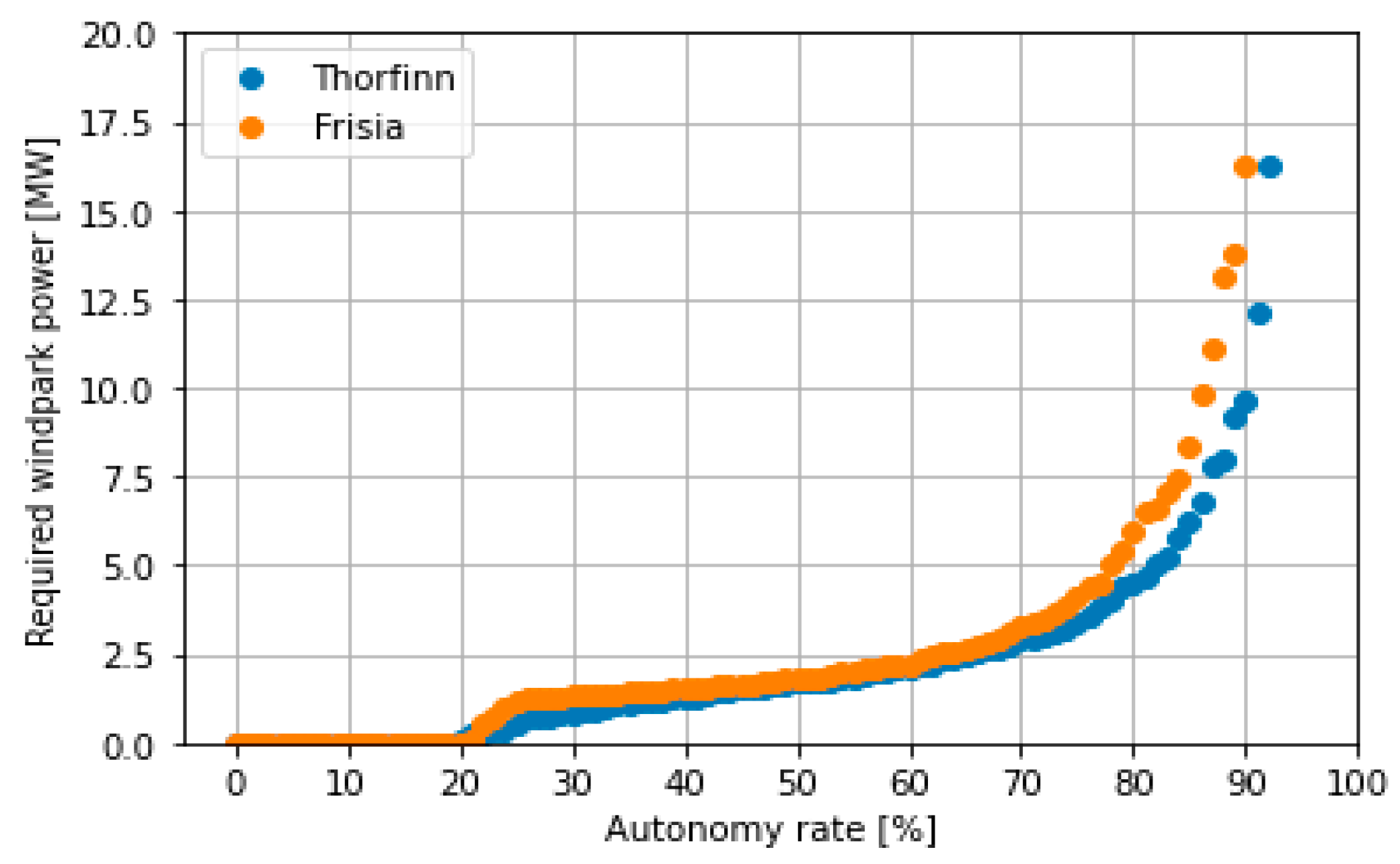
3.3.4. Wind Farm
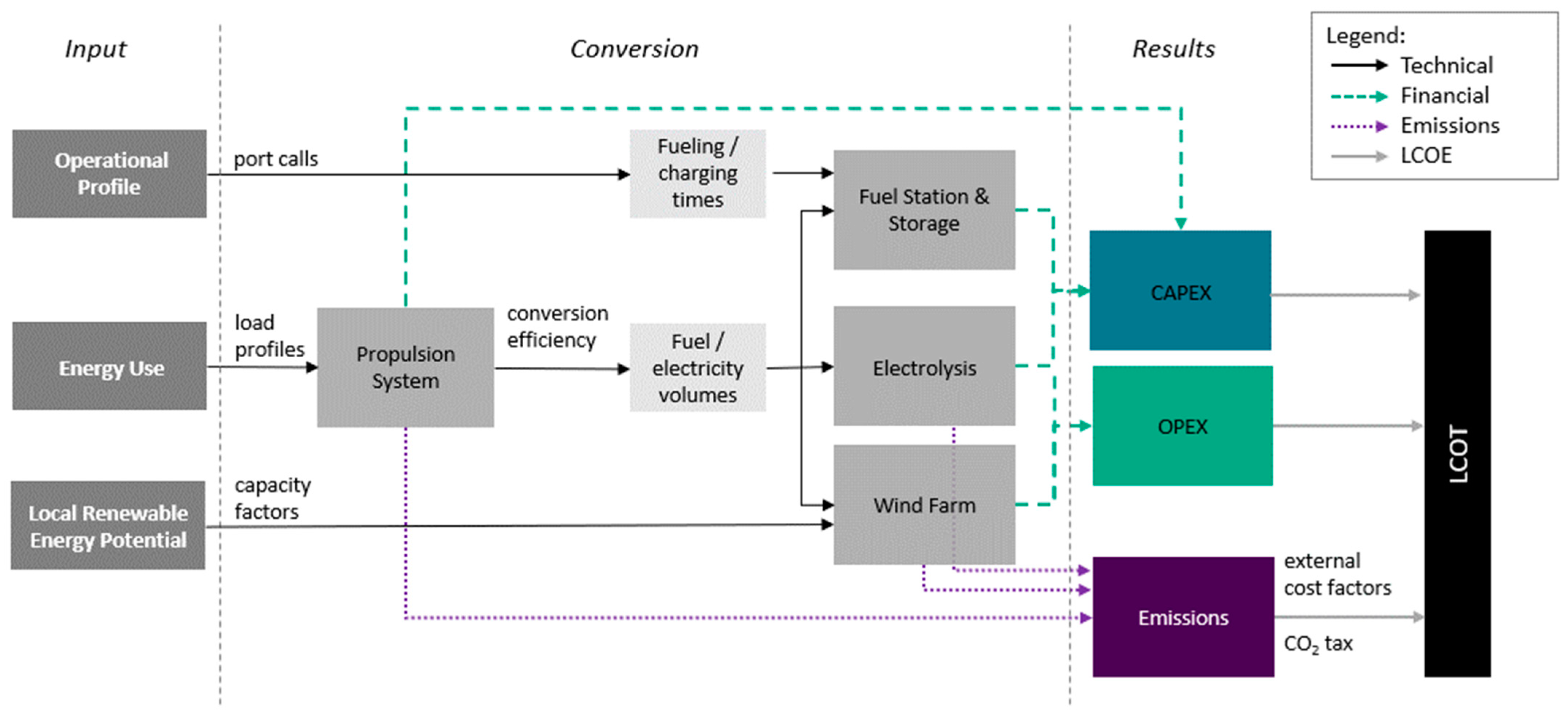
3.3.5. Levelized Costs of Transportation
3.4. Implementation
4. Case Study
4.1. Operational Analysis
4.2. Energy Use Estimation
4.3. Hydrogen Fuel System
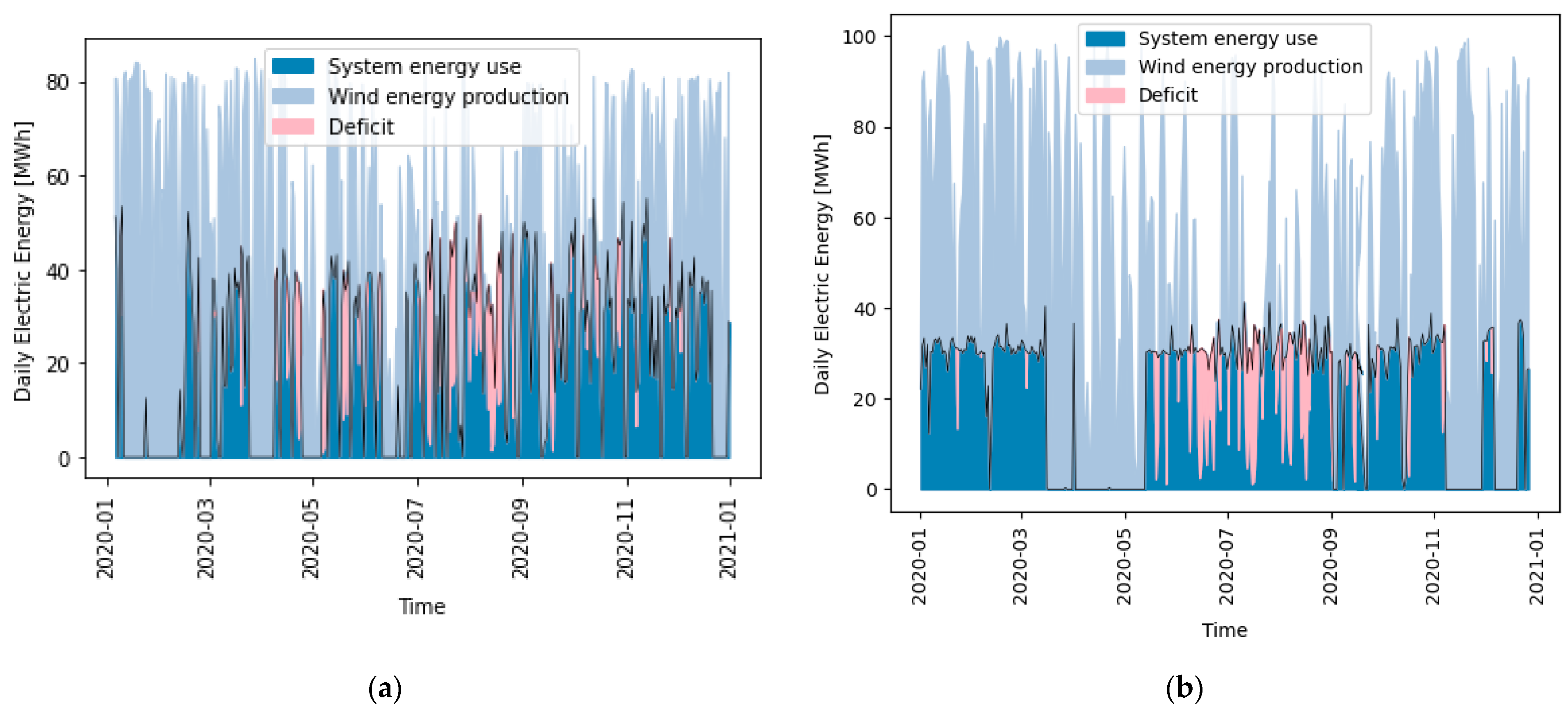
4.3.1. System Sizing and Energy Balance
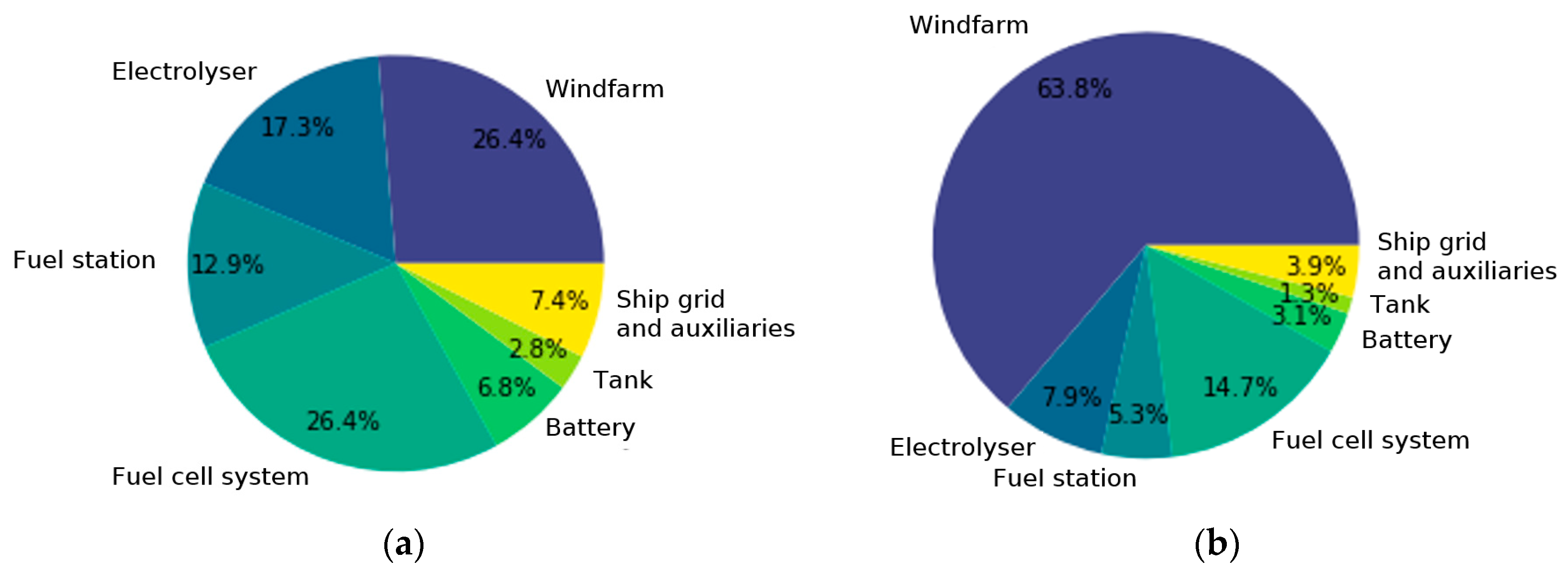
4.3.2. CAPEX, OPEX and Wind Energy Revenues
4.3.3. Emissions
4.3.4. Levelized Costs of Transportation (LCOT)
5. Conclusions
Author Contributions
Funding
Institutional Review Board Statement
Informed Consent Statement
Data Availability Statement
Acknowledgments
Conflicts of Interest
Appendix A

| Ship Technical Parameter | Missing Parameter Replacement |
|---|---|
| MMSI | Mandatory parameters |
| Length overall | |
| Breath | |
| Gross tonnage | |
| Dead weight, reference | |
| Draught, reference | |
| Ship speed, reference | |
| Main engine power, reference | |
| Main engine type (slow/medium/high-speed) | Medium-speed diesel |
| ME model year | 2000 |
| ME fuel type | Heavy fuel oil |
| AE power | statistical |
| AE type | Medium-speed diesel |
| AE model year | 2000 |
| AE fuel type | Marine distillate oil |
| Midship section | statistical |
| Ship Facilities | Comfort Class | At Berth | Ma-Noeuvre | Slow Cruising | Cruising |
|---|---|---|---|---|---|
| Seating area without service | low | 0.46 | 0.67 | 0.55 | 0.28 |
| Seating area with service | medium | 0.535 | 9.745 | 0.625 | 0.38 (+10%) |
| Hoteling facilities | high | 0.61 | 0.82 | 0.7 | 0.48 (+20%) |
| Parameter | Unit | Value | Source/Basis | |
|---|---|---|---|---|
| Emission external costs factors | ||||
| CO2 | EUR/t | 260 | German Environmental Agency 2014 [53]. Medium long-term scenario (until 2050). | |
| NOx | EUR/t | 12,600 | TU Delft 2018 [4] Value for rural areas, as ships spend most of their operation in open water. | |
| PM 2.5 | EUR/t | 7000 | ||
| SOx | EUR/t | 4300 | Sanabra 2014 [54], lowest sensitivity. | |
| Fuel cell propulsion system | ||||
| Degree of hybridization | % | 35 | Aligned to Han 2014 [38] | |
| Li-Ion battery charging efficiency | % | 90 | Valoen 2007 [55] | |
| Li-Ion battery discharging efficiency | % | 85 | ||
| Max. C-Rate discharge | - | 1 | Scenario assumption | |
| Opt. C-Rate charge | - | 0.3 | Scenario assumption | |
| Fuel cell system efficiency | % | 50 | Van Biert 2016, PEM-Fuel cell [56] | |
| Fuel cell load factor at reference speed | % | 70 | Scenario assumption. For optimum range of 40–60% [38], operation at medium speeds. | |
| Hydrogen tank ambient temperature | K | 300 | Scenario assumption for regular ambient temperature | |
| Hydrogen tank pressure | bar | 600 | Current on-road technology Rivard 2019, Table 3 [57] | |
| Compressibility factor at storage conditions | - | 1.38 | Cengel 2008 [58] | |
| Lowest allowable hydrogen tank pressure | bar | 30 | Similar empty tank pressure levels were used in HySeas III [34] and for the modeling of an on-road fueling station by Reddi in 2014 [28]. | |
| Battery min. allowable SOC | % | 30 | Scenario assumption for optimum battery lifetime | |
| Battery vol. energy density | kWh/l | 0.3 | University of Washington 2020 [39] | |
| Battery grav. energy density | kWh/kg | 0.17 | ||
| Fuel cell cost factor | €/kW | 1006 | Estimate based on HySeas III project [34] | |
| Hydrogen tank cost factor | €/kg | 519 | Current on-road technology Rivard 2019, Table 3 [57] | |
| Li-Ion battery cost factor | €/kWh | 266.5 | Cole 2021 [59] | |
| Electric motor cost factor | €/kW | 10.25 | Lipman 1999 [60] | |
| Installation cost factor | % | 20 | Scenario assumption | |
| Fuel Station | ||||
| Tube trailer capacity | kg | 600 | Aliquo 2016 [32] | |
| Days of storage safety | d | 2 | Scenario assumption | |
| Trailer cost factor per tank capacity | €/kg | 500 | Aliquo 2016 [32] | |
| Max. pressure tube trailer | bars | 250 | ||
| Min. pressure tube trailer | bars | 30 | Similar empty tank pressure levels were used in HySeas III and for the modeling of an on-road fueling station by Reddi in 2014 [28,34] | |
| Max. pressure low-pressure storage | bars | 50 | Andersson 2019 [27] | |
| Min. pressure low-pressure storage | bars | 10 | Scenario assumption | |
| Low-pressure storage cost | €/kg | 520 | Parks 2014 [61] | |
| Hydrogen grid pressure | bars | 100 | Scenario assumption | |
| Max. flow rate per dispenser | kg/s | 0.05 | HySeas III project [34] | |
| Compressor isentropic efficiency | % | 80 | Parks 2014 [61] | |
| Hydrogen source pressure | bars | Dependent on storage type. | ||
| Hydrogen target pressure | bars | 650 | Hydrogen ship tank pressure +50 bars | |
| € | Weinert 2005 [62] | |||
| Cooling temperature | K | 253 | Cooling level model for an on-road fueling station by Reddi in 2014 [28]. | |
| Cooler coefficient of performance | % | 90 | Cengel 2008 [58] | |
| Charging facility cost factor | €/kW | 205 | Nicholas 2018 [63] | |
| Fuel Station OPEX factor | %CA-PEX/y | 1 | Scenario assumption. | |
| Fuel station auxiliary systems energy use factor | % | 10 | Scenario assumption. | |
| Electrolysis station | ||||
| PEM Electrolyser efficiency | % | 80 | Kumar 2019 [64] for PEM electrolyser, comparative 70% for Alkaline | |
| Electrolyser availability | % | 75 | Scenario assumption. | |
| Pressure after electrolysis | bar | 15 | Scenario assumption. | |
| Electrolysis auxiliary systems cost factor | % | 10 | Scenario assumption. | |
| OPEX factor | %/y | 1 | Scenario assumption. | |
| Electrolysis auxiliary systems energy use factor | % | 30 | Scenario assumption for energy uses of water purification, temperature management | |
| Wind farm | ||||
| Days in buffer storage pipeline | d | 5 | Scenario assumption. | |
| Minimum self-supply rate | % | 80 | Scenario assumption. | |
| Wind energy feed in spot price | 0.01 EUR/kWh | 3.5 | HySeas III project [34] | |
| Offshore wind energy premium in Germany 2020 | 0.01 EUR/kWh | 13.9 | German Ministry of Economy and Climate Protection [50] | |
| Grid electricity price | 0.01 EUR/kWh | 20 | Scenario assumption. | |
| Wind farm CAPEX factor | EUR/kW | 1237/ 4100 | On-shore Stehly 2018 [65]/Off-shore Voormolen 2016 [66] | |
| Wind farm OPEX factor | EUR/kW/y | 37/ 109 | On-shore Stehly 2018 [65]/Off-shore Voormolen 2016 [66] | |
| CO2 emissions factor for wind energy | g/kWh | 27 | Thomson 2015 [67] | |
Appendix B


References
- European Commission. Roadmap to A Single European Transport Area—Towards a Competitive and Resource Efficient Transport System; COM(2011) 144 Final; European Commission: Brussels, Belgium, 2011; Available online: https://eur-lex.europa.eu/LexUriServ/LexUriServ.do?uri=COM:2011:0144:FIN:en:PDF (accessed on 5 May 2022).
- International Maritime Organization (IMO). Initial IMO Strategy on Reduction of GHG Emissions from Ships; MEPC.304(72): London, UK, 13 April 2018; Available online: https://unfccc.int/sites/default/files/resource/250_IMO%20submission_Talanoa%20Dialogue_April%202018.pdf (accessed on 5 May 2022).
- Reşitoğlu, İ.A.; Altinişik, K.; Keskin, A. The pollutant emissions from diesel-engine vehicles and exhaust aftertreatment systems. Clean Technol. Environ. Policy 2015, 17, 15–27. [Google Scholar] [CrossRef] [Green Version]
- Hoen, A.; Nieuwenhuijse, I.; de Bruyn, S. Health Impacts and Costs of Diesel Emissions in the EU; CE Delft: Delft, The Netherlands, 2018; Available online: https://cedelft.eu/publications/health-impacts-and-costs-of-diesel-emissions-in-the-eu/ (accessed on 5 May 2022).
- Petrospot Ltd. Session 4: Supply chain stakeholders have their say on the energy transition. In Proceedings of the Ship Energy Summit, Online. 8 September 2021. [Google Scholar]
- Gómez Trillos, J.C. HySeas III—Market Potential Analysis of RoPax Ferry Market in Europe; Ref. Ares (2019)7435585; German Aerospace Centre (DLR): Oldenburg, Germany, 2019. [Google Scholar]
- European Commission. THETIS-MRV CO2 Emission Report. Available online: https://mrv.emsa.europa.eu/#public/emission-report (accessed on 1 November 2020).
- Cooper, J. Fuels Europe—Statistical Report 2019; FuelsEurope: Brussels, Belgium, 2019; Available online: https://www.fuelseurope.eu/publication/statistical-report-2019/ (accessed on 5 May 2022).
- Kristensen, H.O.; Psaraftis, H. Energy Demand and Exhaust Gas Emissions of Marine Engines. 2015. Available online: https://www.danishshipping.dk/en/services/beregningsvaerktoejer/download/Basic_Model_Linkarea_Link/806/energy-demand-and-emissions-of-marine-engines-september-2015.pdf (accessed on 5 May 2022).
- Winther, M.; Christensen, J.H.; Plejdrup, M.S.; Ravn, E.S.; Eriksson, F.; Kristensen, H.O. Emission inventories for ships in the arctic based on satellite sampled AIS data. Atmos. Environ. 2014, 91, 1–14. [Google Scholar] [CrossRef]
- Jalkanen, J.-P.; Johansson, L.; Kukkonen, J.; Brink, A.; Kalli, J.; Stipa, T. Extension of an assessment model of ship traffic exhaust emissions for particulate matter and carbon monoxide. Atmos. Chem. Phys. 2012, 12, 2641–2659. [Google Scholar] [CrossRef] [Green Version]
- Jalkanen, J.-P.; Johansson, L.; Kukkonen, J. A comprehensive inventory of the ship traffic exhaust emissions in the Baltic Sea from 2006 to 2009. Ambio 2014, 43, 311–324. [Google Scholar] [CrossRef] [Green Version]
- Jalkanen, J.-P.; Johansson, L.; Kukkonen, J. A comprehensive inventory of ship traffic exhaust emissions in the European sea areas in 2011. Atmos. Chem. Phys. 2016, 16, 71–84. [Google Scholar] [CrossRef] [Green Version]
- International Maritime Organization (IMO). Third IMO Greenhouse Gas Study. 2014. Available online: https://www.imo.org/en/OurWork/Environment/Pages/Greenhouse-Gas-Studies-2014.aspx (accessed on 5 May 2022).
- International Maritime Organization (IMO). Fourth IMO Greenhouse Gas Study. 2020. Available online: https://www.imo.org/en/OurWork/Environment/Pages/Fourth-IMO-Greenhouse-Gas-Study-2020.aspx (accessed on 9 April 2022).
- Hydrogen Council. Path to Hydrogen Competitiveness—A Cost Perspective. 2020. Available online: https://hydrogencouncil.com/wp-content/uploads/2020/01/Path-to-Hydrogen-Competitiveness_Full-Study-1.pdf (accessed on 31 March 2021).
- Aarskog, F.G.; Danebergs, J.; Strømgren, T.; Ulleberg, Ø. Energy and cost analysis of a hydrogen driven high speed passenger ferry. Int. Shipbuild. Prog. 2020, 67, 97–123. [Google Scholar] [CrossRef]
- Waldron Davies, C.; Harnisch, J.; Oswaldo, L.; Mckibbon, S.; Saile, S.; Wagner, F.; Walsh, M. 2006 IPCC Guidelines for National Greenhouse Gas Inventories; IPCC: Geneva, Switzerland, 2006. [Google Scholar]
- Regulations for Carriage of AIS. International Maritime Organization (IMO). Available online: https://www.imo.org/en/OurWork/Safety/Pages/AIS.aspx (accessed on 3 March 2020).
- Anwar, N. Navigation Advanced Mates, Masters, 1st ed.; Seamanship International: Lanarkshire, UK, 2006. [Google Scholar]
- MAN Energy Solutions. Basic Principles of Ship Propulsion; MAN Energy Solutions: Copenhagen, Denmark, 2018; Available online: https://www.man-es.com/docs/default-source/marine/tools/basic-principles-of-ship-propulsion_web_links.pdf?sfvrsn=12d1b886_10 (accessed on 5 May 2022).
- Jalkanen, J.-P.; Brink, A.; Kalli, J.; Pettersson, H.; Kukkonen, J.; Stipa, T. A modelling system for the exhaust emissions of marine traffic and its application in the Baltic Sea area. Atmos. Chem. Phys. 2009, 9, 9209–9223. [Google Scholar] [CrossRef] [Green Version]
- Molland, A.F.; Turnock, S.R.; Hudson, D.A. Ship Resistance and Propulsion: Practical Estimation of Ship Propulsive Power, 2nd ed.; Cambridge University Press: Cambridge, UK, 2017. [Google Scholar]
- German Federal Ministry for Economic Affairs and Energy. The National Hydrogen Strategy. 2020. Available online: https://www.bmwk.de/Redaktion/EN/Publikationen/Energie/the-national-hydrogen-strategy.pdf?__blob=publicationFile&v=6 (accessed on 5 May 2022).
- Dincer, I. Green methods for hydrogen production. Int. J. Hydrogen Energy 2012, 37, 1954–1971. [Google Scholar] [CrossRef]
- Thema, M.; Bauer, F.; Sterner, M. Power-to-Gas: Electrolysis and methanation status review. Renew. Sustain. Energy Rev. 2019, 112, 775–787. [Google Scholar] [CrossRef]
- Andersson, J.; Grönkvist, S. Large-scale storage of hydrogen. Int. J. Hydrogen Energy 2019, 44, 11901–11919. [Google Scholar] [CrossRef]
- Reddi, K.; Elgowainy, A.; Sutherland, E. Hydrogen refueling station compression and storage optimization with tube-trailer deliveries. Int. J. Hydrogen Energy 2014, 39, 19169–19181. [Google Scholar] [CrossRef] [Green Version]
- Carriveau, R.; Ting, D.S.-K. (Eds.) Methane and Hydrogen for Energy Storage; Institution of Engineering and Technology: London, UK, 2016. [Google Scholar]
- Elgowainy, A.; Wang, M.; Joseck, F.; Ward, J. Life-Cycle Analysis of Fuels and Vehicle Technologies. In Encyclopedia of Sustainable Technologies; Elsevier: Amsterdam, The Netherlands, 2017; pp. 317–327. [Google Scholar] [CrossRef]
- German National Grid Agency. Regulierung von Wasserstoffnetzen; German National Grid Agency: Bonn, Germany, 2020; Available online: https://www.bundesnetzagentur.de/SharedDocs/Downloads/DE/Sachgebiete/Energie/Unternehmen_Institutionen/NetzentwicklungUndSmartGrid/Wasserstoff/Konsultationsbericht.pdf?__blob=publicationFile&v=1 (accessed on 5 May 2022).
- Aliquo, J. Advanced Hydrogen Fueling Station Supply: Tube Trailers; U.S. Department of Energy. 2016. Available online: https://www.hydrogen.energy.gov/pdfs/review16/tv028_aliquo_2016_p.pdf (accessed on 31 March 2021).
- Iwan, N. Network Expansion. Available online: https://h2.live/en/ (accessed on 31 March 2021).
- Gómez Trillos, J.C. HySeas III—Written Comunication with Project Personnel; German Aerospace Centre, Institute of Networked Energy Systems: Oldenburg, Germany, 2021. [Google Scholar]
- Moore, R. Color Hybrid: Technology Behind the World’s Largest Plug-In Hybrid Ferry. Available online: https://www.rivieramm.com/news-content-hub/news-content-hub/color-hybrid-technology-behind-the-worldrsquos-largest-plug-in-hybrid-ferry-56251 (accessed on 5 May 2022).
- Tvete, H.A. ReCharge. Analysis of Charging- and Shore Power Infrastructure in Norwegian ports; Hg. v. Det Norske Veritas Germanischer Lloyd (DNV-GL): Oslo, Norway, 2017. [Google Scholar]
- Hansson, J.; Månsson, S.; Brynolf, S.; Grahn, M. Alternative marine fuels: Prospects based on multi-criteria decision analysis involving Swedish stakeholders. Biomass Bioenergy 2019, 126, 159–173. [Google Scholar] [CrossRef]
- Han, J.; Charpentier, J.-F.; Tang, T. An Energy Management System of a Fuel Cell/Battery Hybrid Boat. Energies 2014, 7, 2799–2820. [Google Scholar] [CrossRef] [Green Version]
- University of Washington. Lithium-Ion Battery. Available online: https://www.cei.washington.edu/education/science-of-solar/battery-technology/ (accessed on 31 March 2021).
- Tang, D.; Zio, E.; Yuan, Y.; Zhao, J.; Yan, X. The energy management and optimization strategy for fuel cell hybrid ships. In Proceedings of the 2017 2nd International Conference on System Reliability and Safety (ICSRS 2017), Milan, Italy, 20–22 December 2017; pp. 277–281. [Google Scholar]
- De-Troya, J.J.; Álvarez, C.; Fernández-Garrido, C.; Carral, L. Analysing the possibilities of using fuel cells in ships. Int. J. Hydrogen Energy 2016, 41, 2853–2866. [Google Scholar] [CrossRef]
- Townsin, R.L.; Kwon, Y.J. Approximate formulae for the speed loss due to added resistance in wind and waves. R.I.N.A. Suppl. Pap. 1983, 125, 199. [Google Scholar]
- Blendermann, W. Schiffsform und Windlast: Korrelations- und Regressionsanalyse von Windkanalmessungen am Modell; TUHH Hamburg University of Technology: Hamburg, Germany, 1993. [Google Scholar] [CrossRef]
- Harvald, S.A. (Ed.) Resistance and Propulsion of Ships; Wiley: New York, NY, USA, 1983. [Google Scholar]
- Lackenby, H. The effect of shallow water on ship speed. Nav. Eng. J. 1964, 76, 21–26. [Google Scholar] [CrossRef]
- Prohaska, C.W.; Acevedo, M.L.; Hugues, G.; Kinoshita, M.; Landweber, L.; Lap, A.J.W.; Wieghardt, K. Skin Friction and Turbulence Simulation. In Proceedings of the International Towing Tank Conference (ITTC), Madrid, Spain, 15–23 September 1957; p. 45. [Google Scholar]
- Aertssen, G.; Sluys, M.F.V. Service performance and seakeeping trials on a large containership. R. Inst. Nav. Archit. Trans. 1972, 114, 429–447. [Google Scholar]
- United States Environmental Protection Agency (EPA). Proposal to Designate an Emission Control Area for Nitrogen Oxides, Sulfur Oxides and Particulate Matter; Office of Transportation and Air Quality: Ann Arbor, MI, USA, 2010.
- Haas, S.; Krien, U.; Schachler, B.; Bot, S.; kyri-petrou; Zeli, V.; Shivam, K.; Bosch, S. Wind-Python/Windpowerlib; Silent Improvements, Zenodo: Genève, Switzerland, 2021. [Google Scholar] [CrossRef]
- Bundesministerium für Wirtschaft und Energie, EEG-Vergütung. Available online: https://www.erneuerbare-energien.de/EE/Navigation/DE/Technologien/Windenergie-auf-See/Finanzierung/EEG-Verguetung/eeg-verguetung.html (accessed on 2 December 2021).
- AISHub. Available online: www.aishub.net (accessed on 31 March 2021).
- Kristensen, H.O.; Psaraftis, H. Prediction of Resistance and Propulsion Power of Ro-Ro Ships. 2016. Available online: https://www.danishshipping.dk/en/services/beregningsvaerktoejer/download/Basic_Model_Linkarea_Link/163/wp-2-report-4-resistance-and-propulsion-power.pdf (accessed on 5 May 2022).
- Burger, A. Schätzung der Umweltkosten in den Bereichen Energie und Verkehr; Umeltbundesamt: Dessau-Roßlau, Germany, 2014; Available online: https://www.umweltbundesamt.de/sites/default/files/medien/378/publikationen/hgp_umweltkosten_0.pdf (accessed on 5 May 2022).
- Sanabra, M.C.; Santamaría, J.J.U.; De Osés, F.X.M. Manoeuvring and hotelling external costs: Enough for alternative energy sources? Marit. Policy Manag. 2014, 41, 42–60. [Google Scholar] [CrossRef] [Green Version]
- Valøen, L.O.; Shoesmith, M.; Moli, E.-O. The Effect of PHEV and HEV Duty Cycles on Battery and Battery Pack Performance. In Proceedings of the PHEV 2007 Conference: Where the Grid Meets the Road, Winnipeg, MB, Canada, 1–2 November 2007. [Google Scholar]
- van Biert, L.; Godjevac, M.; Visser, K.; Aravind, P.V. A review of fuel cell systems for maritime applications. J. Power Sour. 2016, 327, 345–364. [Google Scholar] [CrossRef] [Green Version]
- Rivard, E.; Trudeau, M.; Zaghib, K. Hydrogen Storage for Mobility: A Review. Materials 2019, 12, 1973. [Google Scholar] [CrossRef] [Green Version]
- Çengel, Y.A. Thermodynamics: An Engineering Approach; McGraw-Hill Higher Education: Boston, MA, USA, 2008. [Google Scholar]
- Cole, W.; Frazier, A.W.; Augustine, C. NREL/TP-6A20-79236; Cost Projections for Utility-Scale Battery Storage: 2021 Update; National Renewable Energy Laboratory: Golden, CO, USA, 2021.
- Lipman, T.E. The Cost of Manufacturing Electric Vehicle Drivetrains; California Air Resources Board: Davis, CA, USA, 1999.
- Parks, G.; Boyd, R.; Cornish, J.; Remick, R. Hydrogen Station Compression, Storage, and Dispensing Technical Status and Costs: Systems Integration; National Renewable Energy Lab.: Golden, CO, USA, 2014. [CrossRef] [Green Version]
- Weinert, J. A Near-Term Economic Analysis of Hydrogen Fueling Stations; Institute of Transportation Studies, University of California: Davis, CA, USA, 2005. [Google Scholar]
- Nicholas, M.; Hall, D. Lessons Learned on Early Electric Vehicle Fast-Charging Deployments; International Council on Clean Transportation: Washington, DC, USA, 2018; pp. 7–26. Available online: https://theicct.org/sites/default/files/publications/ZEV_fast_charging_white_paper_final.pdf (accessed on 5 May 2022).
- Kumar, S.S.; Himabindu, V. Hydrogen production by PEM water electrolysis—A review. Mater. Sci. Energy Technol. 2019, 2, 442–454. [Google Scholar] [CrossRef]
- Stehly, T.J.; Beiter, P.C. 2018 Cost of Wind Energy Review; National Renewable Energy Lab: Golden, CO, USA, 2020. Available online: https://www.nrel.gov/docs/fy20osti/74598.pdf (accessed on 5 May 2022).
- Voormolen, J.; Junginger, H.; van Sark, W. Unravelling historical cost developments of offshore wind energy in Europe. Energy Policy 2016, 88, 435–444. [Google Scholar] [CrossRef]
- Thomson, C.; Harrison, G. Life Cycle Costs and Carbon Emissions of Offshore Wind Power; ClimateXChange: Edinburgh, UK, 2015; Available online: http://www.climatexchange.org.uk/files/4014/3325/2377/Main_Report_-_Life_Cycle_Costs_and_Carbon_Emissions_of_Offshore_Wind_Power.pdf (accessed on 5 May 2022).


| Speed V | Main Engine Load Factor | Distance to Next Port | State |
|---|---|---|---|
| <1 kn | any | <3 km | at berth |
| >3 km | anchored | ||
| 1 < V > 5 kn | any | <3 km | maneuvering |
| >3 km | open-water maneuvering | ||
| >5 kn | <0.65 | any | slow cruising |
| >0.65 | cruising |
| Unit | Earl Thorfinn | Frisia III | |
|---|---|---|---|
| MMSI | - | 232,000,760 | 211,692,820 |
| Length | M | 45.3 | 74.4 |
| Breath | M | 12.2 | 13.4 |
| Gross Tonnage | Mt | 771 | 1786 |
| Speed | Kn | 12 | 12 |
| Power | kW | 1486 | 1292 |
| Passengers | - | 191 | 1338 |
| Lane-Meters | m | 22 | 120 |
| Vessel | Earl Thorfinn | Frisia III |
|---|---|---|
| Main port | Kirkwall | Norddeich |
| Avg. port calls per day | 1.37 | 4.53 |
| Avg. time in port during operation [hh:mm] | 02:51 | 00:48 |
| Min. time in port outside operation [hh:mm] | 09:42 | 13:10 |
| Sizing Parameter | Earl Thorfinn | Frisia III |
|---|---|---|
| [MW] | 4.0 | 3.4 |
| [MW] | 2.21 | 1.7 |
| [kg] | 1800 | 1246 |
| [MW] | 0.75 | 1.25 |
| [kg] | 882 | 684 |
| Earl Thorfinn | Frisia III | |
|---|---|---|
| Energy produced by wind farm [MWh/y] | 18,474 | 20,164 |
| Hydrogen fuel system total energy use [MWh/y] | 7816 | 7943 |
| Grid purchase [MWh/y] | 1203 | 1053 |
| Grid feed-in [MWh/y] | 11,860 | 13,274 |
| Excess wind energy revenues [M€/y] | +0.174 | +0.254 |
| Scenario Parameter | Earl Thorfinn | Frisia III |
|---|---|---|
| Diesel use base [t/y] | 430 | 468 |
| CO2 mass base [t/y], at 0.260 t€/t | 1409.1 | 1463 |
| NOx mass base [t/y], at 12.6 t€/t | 71.1 | 58.2 |
| SOx base [t/y], at 4.3 t€/t | 0.6 | 0.7 |
| PM2.5 mass base [t/y], at 70.0 t€/t | 1.0 | 1.1 |
| Emission external costs [M€/y] | 1.335 | 1.194 |
| Expected CO2 tax [M€/y] | 0.035 | 0.037 |
| Hydrogen use altern. [t/y] | 111.7 | 114.1 |
| CO2 altern. [t/y], at 0.260 t€/t | 211.0 | 214.4 |
| Emission external costs [M€/y] | 0.055 | 0.056 |
| CO2 tax altern. [M€/y] | 0.005 | 0.005 |
| Hydrogen fuel system external emission cost savings [%] | 95.9% | 95.3% |
| CO2 tax savings [%] | 85.7% | 86.5% |
Publisher’s Note: MDPI stays neutral with regard to jurisdictional claims in published maps and institutional affiliations. |
© 2022 by the authors. Licensee MDPI, Basel, Switzerland. This article is an open access article distributed under the terms and conditions of the Creative Commons Attribution (CC BY) license (https://creativecommons.org/licenses/by/4.0/).
Share and Cite
Fitz, A.C.; Gómez Trillos, J.C.; Sill Torres, F. AIS-Based Estimation of Hydrogen Demand and Self-Sufficient Fuel Supply Systems for RoPax Ferries. Energies 2022, 15, 3482. https://doi.org/10.3390/en15103482
Fitz AC, Gómez Trillos JC, Sill Torres F. AIS-Based Estimation of Hydrogen Demand and Self-Sufficient Fuel Supply Systems for RoPax Ferries. Energies. 2022; 15(10):3482. https://doi.org/10.3390/en15103482
Chicago/Turabian StyleFitz, Annika Christine, Juan Camilo Gómez Trillos, and Frank Sill Torres. 2022. "AIS-Based Estimation of Hydrogen Demand and Self-Sufficient Fuel Supply Systems for RoPax Ferries" Energies 15, no. 10: 3482. https://doi.org/10.3390/en15103482
APA StyleFitz, A. C., Gómez Trillos, J. C., & Sill Torres, F. (2022). AIS-Based Estimation of Hydrogen Demand and Self-Sufficient Fuel Supply Systems for RoPax Ferries. Energies, 15(10), 3482. https://doi.org/10.3390/en15103482